Cavitation during creep-fatigue loading

ABSTRACT

Cavitation is expected to be of equal importance for assessing creep damage during cyclic as during static loading conditions. However, the amount of cavitation data is much more limited in the former case. In particular, two features have been missing: basic models for hysteresis loops and for the formation of cavities during cyclic loading. In this paper, such models are presented and compared with published data for LCF of 1Cr0.5Mo steel. To study the role of the creep–fatigue interaction, the influence of pre-creep as well as LCF cycles with and without hold times were included. Hysteresis loops under these conditions could be well reproduced. A model for nucleation of cavities during creep is adapted to cyclic loading. The total creep strain determined with the help of the loop model could be used to predict the number of cavities during the different LCF loops in an acceptable way.

KEYWORDS:

• Cavitation
• creep-fatigue
• hysteresis loop
• creep damage
• 1Cr0.5Mo

Introduction

Creep and fatigue are common in high-temperature plants. Thermal fatigue due to strains during start-ups and shutdowns frequently occurs. Gas and steam turbines are particularly exposed, but many other types of plants experience cyclic loading. In recent years, the amount of solar and wind power has significantly increased. Since these renewable types of power are weather sensitive, their output varies. This variation has to be supplemented with additional base power, for example from conventional fossil-fired units. These units have to be in standby and are exposed to many more start-ups and thereby also more cyclic loading than in the past.

The role of cyclic loading is traditionally studied with the help of low cycle fatigue (LCF). The temperature is selected to be near the maximum temperature for the component that is investigated [1]. However, it has turned out that this type of testing often underestimates the observed damage in the microstructure. For this reason, thermal-fatigue (TMF) is used instead where both strain and temperature are cycled. It has been demonstrated that the temperature cycle should be as wide as possible including low temperatures to reproduce the observed creep damage [2]. LCF and TMF must include hold times to produce creep damage [3]. The hold time is usually introduced by keeping the strain constant at the maximum or minimum strain in the cycle. An alternative is to have the hold time at constant stress, thereby avoiding the stress relaxation, and this increases the amount of creep damage.

Formation of creep cavities is believed to be of major importance for the initiation of rupture during cyclic loading in the same way as during static conditions. When the cavitation in grain boundaries has reached a critical level, failure takes place in tensile specimens [4]. In components, crack initiation occurs instead [5]. Basic modelling of initiation and growth of cavities during cyclic loading has only been performed to a limited extent [6]. Instead, it has been necessary to rely on modelling for pure creep conditions, where models both for nucleation and growth can represent observations quite well [4].

It is now believed that the main mechanism for the formation of cavities is grain boundary sliding (GBS). This is a natural assumption. Particles in sliding grain boundaries are exposed to shearing stresses that can easily open up cavities. However, even if essentially no particles are present as in pure copper, cavities can be created at grain boundary – subgrain junctions. Lim gave a mechanism for this and showed that this is a thermodynamically feasible process and there is an energy gain when a cavity is formed [7]. With this important result, it was no longer necessary to use classical nucleation theory, and quantitative models could be formulated.

With the help of finite element modelling (FEM), it has been shown that the amount of GBS is proportional to the creep strain [8]. This is also in accordance with observations [9]. The FEM results gave also the proportionality constant. Thus, GBS can quantitatively be predicted and the findings agree with many observations. These results are used in the double ledge model to determine the number of creep cavities [10]. This model has been verified by comparison to experiments for several materials [11].

Models for diffusion-controlled growth of cavities have been available for many years [12]. However, it turned out that these models tended to overestimate the observed growth rates. It was realised that the growth rate could not be faster than the deformation rate of the surrounding material [13], which is referred to as constrained growth. Models taking this effect into account were quickly established [14], but they still tended to overestimate the growth rate. A reanalysis of the growth with the help of FEM has given a new model that is in accordance with observations [15].

Strain controlled growth of creep cavities can also take place. There are a number of models in the literature. However, few take constrained growth into account which can overestimate the growth rate, in particular for larger cavities. For small cavities, the situation can be the opposite. Very limited growth is given for cavity nuclei, making it difficult to use the models for prediction of cavity growth. A new model that relates the growth to the amount of GBS avoids these problems [6] and that will be applied for cyclic loading in the present paper.

It is important to distinguish between ductile and brittle rupture during creep. Ductile rupture is related to ductility exhaustion and to plastic collapse and necking [16]. During cyclic loading brittle rupture is the dominating rupture type. The main mechanism behind brittle rupture is believed to be nucleation, growth and linkage of creep cavities. When the cavitated area fraction in the grain boundaries has reached a certain level, failure takes place. Since quantitative expressions are available for nucleation and growth of cavities, brittle rupture during creep can be predicted. This has been done for a number of austenitic stainless steel [17]. In the modelling, the development of the microstructure must also be described including the dislocation strength, solid solution hardening and precipitation hardening.

In section 2, a basic model for hysteresis loops will be summarised and applied to the ferritic-bainitic steel 1Cr0.5Mo. The reason for choosing this steel is that cavitation data during LCF are available. In section 3 a model for nucleation of cavities during LCF is proposed, and it is shown that it can reproduce the observed number of cavities for the 1Cr0.5Mo steel. Diffusion- and strain-controlled growth of cavities during cyclic loading is analysed in section 4.

Deformation during cyclic loading

Basic model for hysteresis loops

A number of empirical models for describing hysteresis loops can be found in the literature. One of the most common approaches uses the Ramberg-Osgood formula. With empirical models, a good fit to the data is usually easy to obtain. However, there are limitations with this type of model. Typically, many expressions can describe the data accurately, and if they represent different mechanisms, it is difficult to decide if any of the models have physical significance. In addition, it is difficult or impossible to extrapolate the results to new conditions unless a large dataset is available.

Creep models have been formulated that are based on physical principles and do not involve any adjustable parameters, for a survey see [18]. Such models are here referred to as basic. They have successfully been applied to creep, for example for copper, aluminium alloys and austenitic stainless steels. For cyclic deformation, only limited efforts have been performed in this respect. The procedure in [6] will be followed. A brief description is given here. Also, stress strain curves can also be computed with basic models. In particular, the Voce equation can be derived [19]

(1) $\sigma ={\sigma }_y+({\sigma }_{max\mathrm{f}\mathrm{l}\mathrm{o}\mathrm{w}}-{\sigma }_y)(1-e^{-\omega {\epsilon }_{\mathrm{p}\mathrm{l}}/2})$(1)

where $\sigma$ is the applied stress, $ϵ$_pl the plastic strain, $\sigma$_y the yield strength, $\sigma$_{max flow} the maximum flow stress, and $\omega$ the dynamic recovery constant. $\omega$ is the parameter that controls the deviation from a linear work hardening. From Eq. (1)(1) $\sigma ={\sigma }_y+({\sigma }_{max\mathrm{f}\mathrm{l}\mathrm{o}\mathrm{w}}-{\sigma }_y)(1-e^{-\omega {\epsilon }_{\mathrm{p}\mathrm{l}}/2})$(1) , the plastic strain rate can be found

(2) $\frac{d{\epsilon }_{\mathrm{p}\mathrm{l}}}{dt}=\frac{2}{\omega ({\sigma }_{max\mathrm{f}\mathrm{l}\mathrm{o}\mathrm{w}}-\sigma )}\frac{d\sigma }{dt}$(2)

In [20], a basic model for the secondary creep rate ${\dot{\epsilon }}_{sec}$ and its stress dependence h($\sigma$) was derived. Applications of this equation can be found in the survey [18]. It is given in Eqs. (3)(3) $h\left(\sigma \right)=\frac{2b{c}_{\mathrm{L}}}{m_{\mathrm{T}}}\frac{D_{\mathrm{s}\mathrm{e}\mathrm{l}\mathrm{f}0}b{\tau }_L}{k_{\mathrm{B}}T}{\left(\frac{\sigma }{\alpha Gb}\right)}^3{e}^{\frac{\sigma b^3}{k_{\mathrm{B}}T}}{e}^{-\frac{Q_{\mathrm{s}\mathrm{e}\mathrm{l}\mathrm{f}}}{R_{\mathrm{G}}T}\left[1-{\left(\frac{\sigma }{{\sigma }_{\mathrm{i}\mathrm{m}\mathrm{a}\mathrm{x}}}\right)}^2\right]}{e}^{-\frac{Q_{\mathrm{s}\mathrm{o}\mathrm{l}}}{R_{\mathrm{G}}T}}$(3) and (4(4) $\frac{d{\epsilon }_{\mathrm{p}\mathrm{r}\mathrm{i}\mathrm{m}}}{dt}=\frac{d{\epsilon }_{sec}}{dt}=h(\sigma -{\sigma }_{\mathrm{i}})$(4) )

(3) $h\left(\sigma \right)=\frac{2b{c}_{\mathrm{L}}}{m_{\mathrm{T}}}\frac{D_{\mathrm{s}\mathrm{e}\mathrm{l}\mathrm{f}0}b{\tau }_L}{k_{\mathrm{B}}T}{\left(\frac{\sigma }{\alpha Gb}\right)}^3{e}^{\frac{\sigma b^3}{k_{\mathrm{B}}T}}{e}^{-\frac{Q_{\mathrm{s}\mathrm{e}\mathrm{l}\mathrm{f}}}{R_{\mathrm{G}}T}\left[1-{\left(\frac{\sigma }{{\sigma }_{\mathrm{i}\mathrm{m}\mathrm{a}\mathrm{x}}}\right)}^2\right]}{e}^{-\frac{Q_{\mathrm{s}\mathrm{o}\mathrm{l}}}{R_{\mathrm{G}}T}}$(3)

(4) $\frac{d{\epsilon }_{\mathrm{p}\mathrm{r}\mathrm{i}\mathrm{m}}}{dt}=\frac{d{\epsilon }_{sec}}{dt}=h(\sigma -{\sigma }_{\mathrm{i}})$(4)

where T is the absolute temperature, $\sigma$ is the applied stress, D_self0 is the pre-exponential coefficient for self-diffusion, Q_self is the activation energy for self-diffusion, k_B is Boltzmann’s constant, R_G is the gas constant, m_T is the Taylor factor, b is Burger’s vector, $\tau$_L is the dislocation line tension, $\sigma$_imax is the maximum flow stress at ambient temperatures, and c_L is a work hardening constant. Solid solution hardening gives an additional contribution Q_sol to the activation energy. $\sigma$_i takes into account contributions from solid solution hardening and particle hardening. Eqs. (3)(3) $h\left(\sigma \right)=\frac{2b{c}_{\mathrm{L}}}{m_{\mathrm{T}}}\frac{D_{\mathrm{s}\mathrm{e}\mathrm{l}\mathrm{f}0}b{\tau }_L}{k_{\mathrm{B}}T}{\left(\frac{\sigma }{\alpha Gb}\right)}^3{e}^{\frac{\sigma b^3}{k_{\mathrm{B}}T}}{e}^{-\frac{Q_{\mathrm{s}\mathrm{e}\mathrm{l}\mathrm{f}}}{R_{\mathrm{G}}T}\left[1-{\left(\frac{\sigma }{{\sigma }_{\mathrm{i}\mathrm{m}\mathrm{a}\mathrm{x}}}\right)}^2\right]}{e}^{-\frac{Q_{\mathrm{s}\mathrm{o}\mathrm{l}}}{R_{\mathrm{G}}T}}$(3) and (4(4) $\frac{d{\epsilon }_{\mathrm{p}\mathrm{r}\mathrm{i}\mathrm{m}}}{dt}=\frac{d{\epsilon }_{sec}}{dt}=h(\sigma -{\sigma }_{\mathrm{i}})$(4) ) give a stress exponent of 3 at low stresses, but they generate much larger values at high stresses. With a separate analysis that is not included here, it can be shown that the creep rate given by Eq. (4)(4) $\frac{d{\epsilon }_{\mathrm{p}\mathrm{r}\mathrm{i}\mathrm{m}}}{dt}=\frac{d{\epsilon }_{sec}}{dt}=h(\sigma -{\sigma }_{\mathrm{i}})$(4) is valid also in the primary stage, and that is the stage that is relevant for cycling.

The elastic ${\dot{\epsilon }}_{\mathrm{e}\mathrm{l}}$, plastic ${\dot{\epsilon }}_{\mathrm{p}\mathrm{l}}$, and creep strain rate ${\dot{\epsilon }}_{\mathrm{p}\mathrm{r}\mathrm{i}\mathrm{m}}$ contribute to the total strain rate ${\dot{\epsilon }}_{\mathrm{t}\mathrm{o}\mathrm{t}}$ that is usually the controlling parameter during LCF tests

(5) $\frac{d{\epsilon }_{\mathrm{e}\mathrm{l}}}{dt}+\frac{d{\epsilon }_{\mathrm{p}\mathrm{l}}}{dt}+\frac{d{\epsilon }_{\mathrm{p}\mathrm{r}\mathrm{i}\mathrm{m}}}{dt}=\frac{d{\epsilon }_{\mathrm{t}\mathrm{o}\mathrm{t}}}{dt}$(5)

The elastic strain rate ${\dot{\epsilon }}_{\mathrm{e}\mathrm{l}}$ is given by

(6) $\frac{d{\epsilon }_{\mathrm{e}\mathrm{l}}}{dt}=\frac{d\sigma }{dt}\frac{1}{E}$(6)

where E is the elastic modulus. From Eqs. (2)(2) $\frac{d{\epsilon }_{\mathrm{p}\mathrm{l}}}{dt}=\frac{2}{\omega ({\sigma }_{max\mathrm{f}\mathrm{l}\mathrm{o}\mathrm{w}}-\sigma )}\frac{d\sigma }{dt}$(2) , (4(4) $\frac{d{\epsilon }_{\mathrm{p}\mathrm{r}\mathrm{i}\mathrm{m}}}{dt}=\frac{d{\epsilon }_{sec}}{dt}=h(\sigma -{\sigma }_{\mathrm{i}})$(4) ), (5(5) $\frac{d{\epsilon }_{\mathrm{e}\mathrm{l}}}{dt}+\frac{d{\epsilon }_{\mathrm{p}\mathrm{l}}}{dt}+\frac{d{\epsilon }_{\mathrm{p}\mathrm{r}\mathrm{i}\mathrm{m}}}{dt}=\frac{d{\epsilon }_{\mathrm{t}\mathrm{o}\mathrm{t}}}{dt}$(5) ) and (6(6) $\frac{d{\epsilon }_{\mathrm{e}\mathrm{l}}}{dt}=\frac{d\sigma }{dt}\frac{1}{E}$(6) ), the stress rate can be obtained

(7) $\frac{d\sigma }{dt}=\frac{1}{1/E+2/\left[\omega ({\sigma }_{max\mathrm{f}\mathrm{l}\mathrm{o}\mathrm{w}}-sgn({\dot{\epsilon }}_{\mathrm{t}\mathrm{o}\mathrm{t}})\sigma )\right]}\left[\frac{d{\epsilon }_{\mathrm{t}\mathrm{o}\mathrm{t}}}{dt}-h(\sigma -sgn({\dot{\epsilon }}_{\mathrm{t}\mathrm{o}\mathrm{t}}){\sigma }_{\mathrm{i}})\right]$(7)

The sign function sgn in Eq. (7)(7) $\frac{d\sigma }{dt}=\frac{1}{1/E+2/\left[\omega ({\sigma }_{max\mathrm{f}\mathrm{l}\mathrm{o}\mathrm{w}}-sgn({\dot{\epsilon }}_{\mathrm{t}\mathrm{o}\mathrm{t}})\sigma )\right]}\left[\frac{d{\epsilon }_{\mathrm{t}\mathrm{o}\mathrm{t}}}{dt}-h(\sigma -sgn({\dot{\epsilon }}_{\mathrm{t}\mathrm{o}\mathrm{t}}){\sigma }_{\mathrm{i}})\right]$(7) makes the equation valid for both the tension and compression going parts of the loop.

When using Eq. (7)(7) $\frac{d\sigma }{dt}=\frac{1}{1/E+2/\left[\omega ({\sigma }_{max\mathrm{f}\mathrm{l}\mathrm{o}\mathrm{w}}-sgn({\dot{\epsilon }}_{\mathrm{t}\mathrm{o}\mathrm{t}})\sigma )\right]}\left[\frac{d{\epsilon }_{\mathrm{t}\mathrm{o}\mathrm{t}}}{dt}-h(\sigma -sgn({\dot{\epsilon }}_{\mathrm{t}\mathrm{o}\mathrm{t}}){\sigma }_{\mathrm{i}})\right]$(7) , the starting point is to apply creep data and stress–strain curves for monotonous loading. The main parameter that cannot be taken over directly is the dynamic recovery constant $\omega$. The reason is that the dislocations encounter each other much more frequently during cyclic than during static loading. Its value is increased by the ratio between the uniform elongation and the strain range in the LCF test [6]. In the hysteresis loop each half cycle can be assumed to correspond to a static stress-strain test. The resulting expression for $\omega$ is

(8) $\omega (T)=\omega (RT)\frac{{\epsilon }_u}{{\epsilon }_r}{\left[\frac{E(RT)}{E(T)}\right]}^2$(8)

where E is the elastic modulus, $ϵ$_u is the uniform elongation during monotonous loading and $ϵ$_r the strain range during cycling. T and RT represent the values at temperature and room temperature, respectively.

Application to steels

Eq. (7)(7) $\frac{d\sigma }{dt}=\frac{1}{1/E+2/\left[\omega ({\sigma }_{max\mathrm{f}\mathrm{l}\mathrm{o}\mathrm{w}}-sgn({\dot{\epsilon }}_{\mathrm{t}\mathrm{o}\mathrm{t}})\sigma )\right]}\left[\frac{d{\epsilon }_{\mathrm{t}\mathrm{o}\mathrm{t}}}{dt}-h(\sigma -sgn({\dot{\epsilon }}_{\mathrm{t}\mathrm{o}\mathrm{t}}){\sigma }_{\mathrm{i}})\right]$(7) gives a model for a hysteresis loop. The constants in the model are taken from monotonous loading except for the dynamic recovery constant $\omega$ that has to be raised according to Eq. (8)(8) $\omega (T)=\omega (RT)\frac{{\epsilon }_u}{{\epsilon }_r}{\left[\frac{E(RT)}{E(T)}\right]}^2$(8) . An example of the application of Eq. (7)(7) $\frac{d\sigma }{dt}=\frac{1}{1/E+2/\left[\omega ({\sigma }_{max\mathrm{f}\mathrm{l}\mathrm{o}\mathrm{w}}-sgn({\dot{\epsilon }}_{\mathrm{t}\mathrm{o}\mathrm{t}})\sigma )\right]}\left[\frac{d{\epsilon }_{\mathrm{t}\mathrm{o}\mathrm{t}}}{dt}-h(\sigma -sgn({\dot{\epsilon }}_{\mathrm{t}\mathrm{o}\mathrm{t}}){\sigma }_{\mathrm{i}})\right]$(7) is given in Figure 1 for the oxidation-resistant 21Cr11Ni austenitic stainless steel 253 MA. All the steps in the derivation of the loop are made with basic modelling without applying any adjustable parameters.

Figure 1. Hysteresis loop for low cycle fatigue (LCF) of the austenitic stainless steel 253 MA at 750°C. Experimental data from [21] are compared with the model in Eq. (7)(7) $\frac{d\sigma }{dt}=\frac{1}{1/E+2/\left[\omega ({\sigma }_{max\mathrm{f}\mathrm{l}\mathrm{o}\mathrm{w}}-sgn({\dot{\epsilon }}_{\mathrm{t}\mathrm{o}\mathrm{t}})\sigma )\right]}\left[\frac{d{\epsilon }_{\mathrm{t}\mathrm{o}\mathrm{t}}}{dt}-h(\sigma -sgn({\dot{\epsilon }}_{\mathrm{t}\mathrm{o}\mathrm{t}}){\sigma }_{\mathrm{i}})\right]$(7) .

Further examples of computed hysteresis loops from basic creep models are given in [6]. To obtain an acceptable loop the raised value of $\omega$ is essential. Otherwise, the loop has a tendency to look like a parallelogram.

Cavitation will be studied for the ferritic-bainitic 1Cr0.5Mo steel during LCF. To model the cavitation, LCF data and hysteresis loops must be possible to describe. Since no basic creep model is available for this steel, an empirical description is derived from creep rupture data [22]. An Arrhenius expression for the rupture time t_R is fitted to the data.

(9) $\frac{1}{t_{\mathrm{R}}}=C_{\mathrm{R}}exp(-\frac{Q_{\mathrm{R}}}{k_{\mathrm{B}}T}){\sigma }^{n_{\mathrm{N}}}$(9)

The fit is illustrated in Figure 2.

Figure 2. Creep rupture data for 1Cr0.5Mo steel [22] fitted to the Arrhenius expression in Eq. (9)(9) $\frac{1}{t_{\mathrm{R}}}=C_{\mathrm{R}}exp(-\frac{Q_{\mathrm{R}}}{k_{\mathrm{B}}T}){\sigma }^{n_{\mathrm{N}}}$(9) .

The data for stresses above 300 MPa are not taken into account since they are not needed for the hysteresis loops. The resulting values of the parameters are Q_R = 391 kJ/mol, n_N = 4.4 and C_R = 1.0 × 10¹² with the rupture time t_R in hours. With the Monkman–Grant relation, the strain rate is obtained.

(10) $\dot{\epsilon }=\frac{{\epsilon }_{\mathrm{R}}}{t_{\mathrm{R}}}$(10)

The rupture ductility $ϵ$_R is given a value of 0.1. No attempt will be made here to derive a basic model for rupture during LCF. The well-established Coffin-Manson equation will be used

(11) $N_{\mathrm{i}\mathrm{n}\mathrm{i}\mathrm{t}}=C_{\mathrm{C}\mathrm{M}}(\mathrm{\Delta }{\epsilon }_{\mathrm{p}\mathrm{l}}{)}^{-{\beta }_{\mathrm{C}\mathrm{M}}}$(11)

where N_init is the number of cycles to crack initiation, ∆$ϵ$_pl the plastic strain range in the load cycle; C_CM and $\beta$_CM are parameters that are fitted to the observations. In Figure 3, the plastic strain is shown as a function of the number of cycles to crack initiation. Sometimes the same relation can also be used for the total and the elastic strain ranges. This is the case in Figure 3.

Figure 3. Relation between the number of cycles to crack initiation and the total, plastic and elastic strain ranges for 1Cr0.5Mo. Experimental data from [23]. CC stands for continuous cycling (without hold times).

With the help of Eq. (7)(7) $\frac{d\sigma }{dt}=\frac{1}{1/E+2/\left[\omega ({\sigma }_{max\mathrm{f}\mathrm{l}\mathrm{o}\mathrm{w}}-sgn({\dot{\epsilon }}_{\mathrm{t}\mathrm{o}\mathrm{t}})\sigma )\right]}\left[\frac{d{\epsilon }_{\mathrm{t}\mathrm{o}\mathrm{t}}}{dt}-h(\sigma -sgn({\dot{\epsilon }}_{\mathrm{t}\mathrm{o}\mathrm{t}}){\sigma }_{\mathrm{i}})\right]$(7) , hysteresis loops for 1Cr0.5Mo can now be modelled. Results for two cycles without hold time are given in Figure 4. The experimental data refer to mid-life cycles. The computed cycles were run for the experimental mid-life data until the cycles had been stabilised. In Figure 4a, a cycle for tempered condition is shown. In Figure 4b, the specimen has been exposed to 5% creep strain at 600ºC before the LCF testing. As can be seen, the effect of this pre-creep is that the maximum stress in the loop is reduced probably due to softening of the microstructure during creep.

Figure 4. Hysteresis loop for low cycle fatigue (LCF) of the ferritic-bainitic steel 1Cr0.5Mo at 535ºC. Experimental data from [23] are compared with the model in Eq. (7)(7) $\frac{d\sigma }{dt}=\frac{1}{1/E+2/\left[\omega ({\sigma }_{max\mathrm{f}\mathrm{l}\mathrm{o}\mathrm{w}}-sgn({\dot{\epsilon }}_{\mathrm{t}\mathrm{o}\mathrm{t}})\sigma )\right]}\left[\frac{d{\epsilon }_{\mathrm{t}\mathrm{o}\mathrm{t}}}{dt}-h(\sigma -sgn({\dot{\epsilon }}_{\mathrm{t}\mathrm{o}\mathrm{t}}){\sigma }_{\mathrm{i}})\right]$(7) . a) Tempered condition; b) Pre-crept to 5% strain at 600ºC.

The influence of a hold time of 5 min is illustrated in Figure 5. In the same way as in Figure 4, a comparison is made between LCF with and without pre-creep. In Figure 5b, the pre-creep was performed at 560ºC. The inclusion of a hold time reduces the maximum stress in the loop further, which can be seen by comparing Figures 4 and 5. The same constants have been used to derive both figures. The only difference is that the creep strain in the hold time is taken into account in Figure 5 as well. The differences between a) and b) in Figures 4 and 5 are simply due to the influence of pre-creep. It is evident that the model in Eq. (7)(7) $\frac{d\sigma }{dt}=\frac{1}{1/E+2/\left[\omega ({\sigma }_{max\mathrm{f}\mathrm{l}\mathrm{o}\mathrm{w}}-sgn({\dot{\epsilon }}_{\mathrm{t}\mathrm{o}\mathrm{t}})\sigma )\right]}\left[\frac{d{\epsilon }_{\mathrm{t}\mathrm{o}\mathrm{t}}}{dt}-h(\sigma -sgn({\dot{\epsilon }}_{\mathrm{t}\mathrm{o}\mathrm{t}}){\sigma }_{\mathrm{i}})\right]$(7) can describe the hysteresis loops for 1Cr0.5Mo in an acceptable way.

Figure 5. Hysteresis loop for low cycle fatigue (LCF) of the bainitic steel 1Cr0.5Mo at 535ºC with a hold time of 5 min. Experimental data from [23] are compared with the model in Eq. (7)(7) $\frac{d\sigma }{dt}=\frac{1}{1/E+2/\left[\omega ({\sigma }_{max\mathrm{f}\mathrm{l}\mathrm{o}\mathrm{w}}-sgn({\dot{\epsilon }}_{\mathrm{t}\mathrm{o}\mathrm{t}})\sigma )\right]}\left[\frac{d{\epsilon }_{\mathrm{t}\mathrm{o}\mathrm{t}}}{dt}-h(\sigma -sgn({\dot{\epsilon }}_{\mathrm{t}\mathrm{o}\mathrm{t}}){\sigma }_{\mathrm{i}})\right]$(7) . a) Tempered condition; b) Pre-crept to 5% strain at 560ºC.

Nucleation of cavities

Nucleation mechanism

It is assumed that the formation of creep cavities is based on the same principles for static and cyclic loading. A survey of the basic models for cavitation is given in [4]. The starting point is that the cavities are formed in sliding grain boundaries at particles or at grain boundary-subboundary junctions. Mechanisms other than grain boundary sliding (GBS) for the creation of cavities have been proposed, but they do not seem to be in agreement with observations. The amount of GBS u_GBS is directly proportional to the creep strain

(12) $u_{\mathrm{G}\mathrm{B}\mathrm{S}}=C_{\mathrm{s}}\epsilon$(12)

With the help of FEM modelling [24], the value of the proportionality constant C_s has been determined

(13) $C_{\mathrm{s}}={\dot{u}}_{\mathrm{G}\mathrm{B}\mathrm{S}}/\dot{\epsilon }=\frac{3\varphi }{2\xi }{d}_{\mathrm{g}\mathrm{r}\mathrm{a}\mathrm{i}\mathrm{n}}$(13)

where d_grain is the grain size, $\varphi$ = 0.15 to 0.33 (the value increases with the creep stress exponent) and $\xi$≈1.4 are constants.

To describe that the nucleation rate is proportional to the creep rate, the double ledge model is used [10]. According to this model, a cavity can be formed when a particle meets a subboundary or a subboundary meets another subboundary in a sliding grain boundary

(14) $\frac{d{n}_{\mathrm{c}\mathrm{a}\mathrm{v}}}{dt}=\frac{0.9C_s}{d_{\mathrm{s}\mathrm{u}\mathrm{b}}}(\frac{g_{\mathrm{s}\mathrm{u}\mathrm{b}}}{d_{\mathrm{s}\mathrm{u}\mathrm{b}}^2}+\frac{g_{\mathrm{p}\mathrm{a}\mathrm{r}\mathrm{t}}}{{\lambda }^2})\dot{\epsilon }=B_{\mathrm{s}}\dot{\epsilon }$(14)

where n_cav is the number of cavities nucleated per unit grain boundary area, and d_sub is the subgrain diameter, which is inversely proportional to the dislocation stress. $\lambda$ is the interparticle spacing in the grain boundary. g_part and g_sub are the fractions of particles and subboundary junctions where cavitation takes place. The factor 0.9 is due to averaging over different orientations. The validity of the equation has been verified for copper [25] and austenitic stainless steels [11].

The model for cavitation will be compared to data for LCF for the 1Cr0.5Mo steel [23]. The cavitation in this type of ferritic-bainitic steel appears in a similar way to that in fcc alloys with the important difference that the cavities are present in prior austenitic grain boundaries in the ferritic-bainitic steels, whereas they are located in the ordinary grain boundaries in fcc alloys.

Application to creep

To study the combined influence of creep and fatigue, some specimens were exposed to creep before the LCF testing. The creep testing was carried out at 560 or 600ºC at 100 MPa until a creep strain of 5% was reached.

The cavitation during the creep phase will first be considered. Since this phase only involves creep, Eq. (14)(14) $\frac{d{n}_{\mathrm{c}\mathrm{a}\mathrm{v}}}{dt}=\frac{0.9C_s}{d_{\mathrm{s}\mathrm{u}\mathrm{b}}}(\frac{g_{\mathrm{s}\mathrm{u}\mathrm{b}}}{d_{\mathrm{s}\mathrm{u}\mathrm{b}}^2}+\frac{g_{\mathrm{p}\mathrm{a}\mathrm{r}\mathrm{t}}}{{\lambda }^2})\dot{\epsilon }=B_{\mathrm{s}}\dot{\epsilon }$(14) should be directly applicable. The results are illustrated in Figure 6.

Figure 6. Number of cavities versus creep strain for specimens later used in LCF testing. Experimental data from [23] are compared with the model in Eq. (14)(14) $\frac{d{n}_{\mathrm{c}\mathrm{a}\mathrm{v}}}{dt}=\frac{0.9C_s}{d_{\mathrm{s}\mathrm{u}\mathrm{b}}}(\frac{g_{\mathrm{s}\mathrm{u}\mathrm{b}}}{d_{\mathrm{s}\mathrm{u}\mathrm{b}}^2}+\frac{g_{\mathrm{p}\mathrm{a}\mathrm{r}\mathrm{t}}}{{\lambda }^2})\dot{\epsilon }=B_{\mathrm{s}}\dot{\epsilon }$(14) .

The nucleation of cavities is assumed to take place at particles in the grain boundaries. From the micrographs, it could be found that the average spacing between particles was $\lambda$ = 5 µm and that one particle out of five formed a cavity. This implies that g_part is 0.2. The value of g_part is not possible to predict. The grain size d_grain was 12 µm and the creep exponent n_N = 4.4. From Eq. (13)(13) $C_{\mathrm{s}}={\dot{u}}_{\mathrm{G}\mathrm{B}\mathrm{S}}/\dot{\epsilon }=\frac{3\varphi }{2\xi }{d}_{\mathrm{g}\mathrm{r}\mathrm{a}\mathrm{i}\mathrm{n}}$(13) a value of C_s = 2.5 µm is then obtained. These constants are also used when interpreting the results from the LCF tests.

The number of cavities in Figure 6 is clearly higher for creep at 560ºC than at 600ºC. This is interpreted as an effect of particle coarsening. Since no basic creep model is available for the 1Cr0.5Mo steel, the difference has to be estimated indirectly. Using Norton equations, the creep rates ${\dot{\epsilon }}_{560}$ at 560 and ${\dot{\epsilon }}_{600}$ at 600ºC can be formulated as

(15) ${\dot{\epsilon }}_{560}=A_{N}exp(-Q_{\mathrm{c}\mathrm{r}\mathrm{e}\mathrm{e}\mathrm{p}}/R_{\mathrm{G}}{T}_{560})(\sigma -{\sigma }_{\mathrm{p}560}{)}^{n_{\mathrm{N}}}$(15)

(16) ${\dot{\epsilon }}_{600}=A_{\mathrm{N}}exp(-Q_{\mathrm{c}\mathrm{r}\mathrm{e}\mathrm{e}\mathrm{p}}/R_{\mathrm{G}}{T}_{600})(\sigma -{\sigma }_{\mathrm{p}600}{)}^{n_{\mathrm{N}}}$(16)

The ratio between the creep rates at 600ºC and 560ºC has been measured and is 21.3. The activation energy Q_creep = 391 kJ/mol and the stress exponent n_N = 4.4 are known, and consequently the ratio between the particle strengths $\sigma$_p560 and $\sigma$_p600 at 560 and 600ºC can be computed from Eqs. (15)(15) ${\dot{\epsilon }}_{560}=A_{N}exp(-Q_{\mathrm{c}\mathrm{r}\mathrm{e}\mathrm{e}\mathrm{p}}/R_{\mathrm{G}}{T}_{560})(\sigma -{\sigma }_{\mathrm{p}560}{)}^{n_{\mathrm{N}}}$(15) and (16(16) ${\dot{\epsilon }}_{600}=A_{\mathrm{N}}exp(-Q_{\mathrm{c}\mathrm{r}\mathrm{e}\mathrm{e}\mathrm{p}}/R_{\mathrm{G}}{T}_{600})(\sigma -{\sigma }_{\mathrm{p}600}{)}^{n_{\mathrm{N}}}$(16) ). The result is that the particle strengthening at 600ºC is 70% of that at 560ºC. This is considered to be due to a difference in particle spacing and that is what is assumed in Figure 6. It can be seen from Figure 6 that the model can represent the number of cavities at 5% creep strain quite well. Since the number of cavities is known to be linear in the creep strain, the strain dependence can also be given in Figure 6 [4].

Application to LCF

LCF tests were performed for the 1Cr0.5Mo steel at 535ºC [23]. Both tests with and without a hold time of 5 min were included. The number of creep cavities was measured before and after the tests. Only in tests with hold time a significant change in the number of cavities was observed. The analysis will be concentrated to those tests. Some of the tests were pre-crept at 560ºC to 5% strain. In total, seven tests with hold time were carried out. The tests were strain controlled. Characteristics for these tests are listed in Table 1.

Table 1. Data for hysteresis loops with hold time of 5 min for 1Cr0.5Mo.

Pre-creep	${ϵ}_{\text{tot}}$, %	${\sigma }_{\text{range}}$ MPa	Ncycl	Ninit	ncav 1/mm^2	$\mathrm{\Delta }\sigma$hold MPa	$\mathrm{\Delta }{ϵ}_{\text{hold}}$ ×10^−2 %	$\mathrm{\Delta }{ϵ}_{\text{cr\_tens}}$ ×10^−4 %	$\mathrm{\Delta }{ϵ}_{\text{cr\_compr}}$ ×10^−4 %
No	0.92	590	720	540	905	62	4.5	6.2	−8.2
No	0.64	559	1590	1283	1097	52	3.8	2.8	−4.4
No	1.2	655	490	348	173	86	6.3	9.7	−13
No	1.53	669	409	334	1156	91	6.7	14	−18
Yes	0.55	447	1710	1489	3202	60	4.4	4.3	−6.5
Yes	0.83	494	671	568	3359	79	5.8	9.1	−14
Yes	1.11	502	576	517	2233	82	6.0	15	−21

Experimental data from the tests are given in the six left most columns in Table 1: total strain range $ϵ$_tot, stress range $\sigma$_range, number of cycles to failure N_cycl, number of cycles to crack initiation N_init, and the number of measured cavities per unit area n_cav after the test. Creep values for the loops have been computed with the help of Eq. (7)(7) $\frac{d\sigma }{dt}=\frac{1}{1/E+2/\left[\omega ({\sigma }_{max\mathrm{f}\mathrm{l}\mathrm{o}\mathrm{w}}-sgn({\dot{\epsilon }}_{\mathrm{t}\mathrm{o}\mathrm{t}})\sigma )\right]}\left[\frac{d{\epsilon }_{\mathrm{t}\mathrm{o}\mathrm{t}}}{dt}-h(\sigma -sgn({\dot{\epsilon }}_{\mathrm{t}\mathrm{o}\mathrm{t}}){\sigma }_{\mathrm{i}})\right]$(7) . In the right most four columns, these values are given: stress drops due to relaxation during the hold time $\mathrm{\Delta }$$\sigma$_hold, amount of creep strain during the hold time $\mathrm{\Delta }$$ϵ$_hold, amount of creep strain during the tension going part of the cycle $\mathrm{\Delta }ϵ$_{cr_tens} (excluding the strain during the hold time), and amount of creep strain during the compression going part of the cycle $\mathrm{\Delta }$$ϵ$_{cr_cmpr}. The amount of stress relaxation during the hold time varied from 50 to 90 MPa, corresponding to creep strains between 0.00038 and 0.00067. Only the first of these parameters can be compared to the experiments. It was shown in section 2.2 that this could successfully be accomplished. The creep strains during the tension and compression going part of the cycle are about two orders of magnitude smaller. In addition, the creep strains in the tension and compression going part of the cycle cancel each other to quite some extent since they have opposite signs. Evidently, the main part of creep strain appears during the hold time.

The prediction of the number of cavities is derived from Eq. (14)(14) $\frac{d{n}_{\mathrm{c}\mathrm{a}\mathrm{v}}}{dt}=\frac{0.9C_s}{d_{\mathrm{s}\mathrm{u}\mathrm{b}}}(\frac{g_{\mathrm{s}\mathrm{u}\mathrm{b}}}{d_{\mathrm{s}\mathrm{u}\mathrm{b}}^2}+\frac{g_{\mathrm{p}\mathrm{a}\mathrm{r}\mathrm{t}}}{{\lambda }^2})\dot{\epsilon }=B_{\mathrm{s}}\dot{\epsilon }$(14) . The important variable is the total creep strain, which is the creep strain in each cycle multiplied by the number of cycles N_cycl. The three contributions in each cycle are as follows: i) from the hold time $\mathrm{\Delta }$$ϵ$_hold, ii) from the compression going part of the cycle $\mathrm{\Delta }$$ϵ$_{cr_cmpr} and iii) from the tension going part $\mathrm{\Delta }$$ϵ$_{cr_tens}. These three contributions are simply added. The following formula for the number of cavities n_cav is obtained.

(17) $n_{cav}=B_{\mathrm{s}}(1-f_{\mathrm{c}\mathrm{l}\mathrm{o}\mathrm{s}\mathrm{e}})(\mathrm{\Delta }{\epsilon }_{\mathrm{h}\mathrm{o}\mathrm{l}\mathrm{d}}+\mathrm{\Delta }{\epsilon }_{\mathrm{c}\mathrm{r}\mathrm{\_}\mathrm{t}\mathrm{e}\mathrm{n}\mathrm{s}}+\mathrm{\Delta }{\epsilon }_{\mathrm{c}\mathrm{r}\mathrm{\_}\mathrm{c}\mathrm{m}\mathrm{p}\mathrm{r}})N_{\mathrm{c}\mathrm{y}\mathrm{c}\mathrm{l}}$(17)

In Eq. (17)(17) $n_{cav}=B_{\mathrm{s}}(1-f_{\mathrm{c}\mathrm{l}\mathrm{o}\mathrm{s}\mathrm{e}})(\mathrm{\Delta }{\epsilon }_{\mathrm{h}\mathrm{o}\mathrm{l}\mathrm{d}}+\mathrm{\Delta }{\epsilon }_{\mathrm{c}\mathrm{r}\mathrm{\_}\mathrm{t}\mathrm{e}\mathrm{n}\mathrm{s}}+\mathrm{\Delta }{\epsilon }_{\mathrm{c}\mathrm{r}\mathrm{\_}\mathrm{c}\mathrm{m}\mathrm{p}\mathrm{r}})N_{\mathrm{c}\mathrm{y}\mathrm{c}\mathrm{l}}$(17) , the constant B_s appears which takes the same value as for the static creep loading, Section 3.2. Some cavities are expected to close during the compression part of the load cycle. This is taken into account with the help of the constant f_close. The value of f_close is analysed in Section 4. A continuous nucleation of cavities is assumed. The number of cavities in Eq. (17)(17) $n_{cav}=B_{\mathrm{s}}(1-f_{\mathrm{c}\mathrm{l}\mathrm{o}\mathrm{s}\mathrm{e}})(\mathrm{\Delta }{\epsilon }_{\mathrm{h}\mathrm{o}\mathrm{l}\mathrm{d}}+\mathrm{\Delta }{\epsilon }_{\mathrm{c}\mathrm{r}\mathrm{\_}\mathrm{t}\mathrm{e}\mathrm{n}\mathrm{s}}+\mathrm{\Delta }{\epsilon }_{\mathrm{c}\mathrm{r}\mathrm{\_}\mathrm{c}\mathrm{m}\mathrm{p}\mathrm{r}})N_{\mathrm{c}\mathrm{y}\mathrm{c}\mathrm{l}}$(17) is proportional to the accumulated creep strain during cycling.

In the modelling, the same parameter values as in Figure 6 have been applied: C_s = 2.5 µm and d_grain = 12 µm. The average stress in the tension and in compression going part of the cycle has been used to determine the subgrain diameter d_sub. The results were about d_sub = 2 µm. Results for the number of cavities are shown in Figure 7 and Figure 8. The number of cavities found experimentally and by modelling during the pre-creep has been added to the result in Figure 8. It can be concluded that the model gives acceptable findings for most of the specimens.

Figure 7. Number of cavities versus number of cycles after LCF testing of 1Cr0.5Mo steels at 535ºC with 5 min hold time in the cycle. Total strain ranges between 0.64 and 1.53%, Experimental data from [23] are compared with the model in Eq. (17)(17) $n_{cav}=B_{\mathrm{s}}(1-f_{\mathrm{c}\mathrm{l}\mathrm{o}\mathrm{s}\mathrm{e}})(\mathrm{\Delta }{\epsilon }_{\mathrm{h}\mathrm{o}\mathrm{l}\mathrm{d}}+\mathrm{\Delta }{\epsilon }_{\mathrm{c}\mathrm{r}\mathrm{\_}\mathrm{t}\mathrm{e}\mathrm{n}\mathrm{s}}+\mathrm{\Delta }{\epsilon }_{\mathrm{c}\mathrm{r}\mathrm{\_}\mathrm{c}\mathrm{m}\mathrm{p}\mathrm{r}})N_{\mathrm{c}\mathrm{y}\mathrm{c}\mathrm{l}}$(17) .

Figure 8. Number of cavities versus number of cycles after LCF testing of 1Cr0.5Mo steels at 535ºC with 5 min hold time in the cycle. Total strain ranges between 0.55 and 1.11%. The specimens were exposed to 5% creep strain before the LCF testing. Experimental data from [23] are compared with the model in Eq. (17)(17) $n_{cav}=B_{\mathrm{s}}(1-f_{\mathrm{c}\mathrm{l}\mathrm{o}\mathrm{s}\mathrm{e}})(\mathrm{\Delta }{\epsilon }_{\mathrm{h}\mathrm{o}\mathrm{l}\mathrm{d}}+\mathrm{\Delta }{\epsilon }_{\mathrm{c}\mathrm{r}\mathrm{\_}\mathrm{t}\mathrm{e}\mathrm{n}\mathrm{s}}+\mathrm{\Delta }{\epsilon }_{\mathrm{c}\mathrm{r}\mathrm{\_}\mathrm{c}\mathrm{m}\mathrm{p}\mathrm{r}})N_{\mathrm{c}\mathrm{y}\mathrm{c}\mathrm{l}}$(17) .

Cavity growth

Diffusion and strain controlled growth

The first to derive an expression for diffusion-controlled growth of cavities were Hull and Rimmer. Their expression was later modified to turn it into a more practical form [12]

(18) $\frac{d{R}_{\mathrm{c}\mathrm{a}\mathrm{v}}}{dt}=2D_0{K}_f(\sigma -{\sigma }_0)\frac{1}{{R_{\mathrm{c}\mathrm{a}\mathrm{v}}}^2}$(18)

where R_cav is the cavity radius in the grain boundary plane, dR_cav/dt its growth rate, $\alpha$ the sintering stress, 2$\gamma$_s sin(α)/R_cav, where $\gamma$_s is the surface energy of the cavity per unit area, and $\alpha$ the cavity tip angle. D_GB the grain boundary self-diffusion coefficient, $\delta$ the grain boundary width, and Ω_a the atomic volume are combined into a grain boundary diffusion parameter D₀, D₀=δD_GBΩ_a/k_BT. k_B is the Boltzmann’s constant and T the absolute temperature. K_f≈0.2 is a constant that depends on the cavitated area fraction. For very small cavities, the sintering stress $\sigma$₀ can be larger than the applied stress $\sigma$ with the consequence that these cavities will shrink and eventually disappear.

It is well known that Eq. (18)(18) $\frac{d{R}_{\mathrm{c}\mathrm{a}\mathrm{v}}}{dt}=2D_0{K}_f(\sigma -{\sigma }_0)\frac{1}{{R_{\mathrm{c}\mathrm{a}\mathrm{v}}}^2}$(18) often overestimates the growth rates [4]. This problem was solved by introducing the requirement that the growth rate cannot be faster than the creep rate of the surrounding matrix [13]. This is referred to as constrained growth in contrast to Eq. (18)(18) $\frac{d{R}_{\mathrm{c}\mathrm{a}\mathrm{v}}}{dt}=2D_0{K}_f(\sigma -{\sigma }_0)\frac{1}{{R_{\mathrm{c}\mathrm{a}\mathrm{v}}}^2}$(18) that represents unconstrained growth. However, for cyclic loading the creep strains are quite small as illustrated in Table 1. It seems quite unlikely that an equilibrium between the growth and the creep rates can be established, which is the requirement for constrained growth. Thus, it must be assumed that the cavity growth is unconstrained during LCF.

Plastic straining can give rise to cavity growth in addition to diffusion. The model for strain-induced growth is taken from [6]. It gives meaningful values also for small cavities

(19) $R_{\mathrm{c}\mathrm{a}\mathrm{v}}=C_{\mathrm{s}}\epsilon$(19)

It simply relates the cavity size to the amount of GBS. This is obvious by comparing Eqs. (12)(12) $u_{\mathrm{G}\mathrm{B}\mathrm{S}}=C_{\mathrm{s}}\epsilon$(12) and (19(19) $R_{\mathrm{c}\mathrm{a}\mathrm{v}}=C_{\mathrm{s}}\epsilon$(19) ). The constant C_s is again given by Eq. (13)(13) $C_{\mathrm{s}}={\dot{u}}_{\mathrm{G}\mathrm{B}\mathrm{S}}/\dot{\epsilon }=\frac{3\varphi }{2\xi }{d}_{\mathrm{g}\mathrm{r}\mathrm{a}\mathrm{i}\mathrm{n}}$(13) . Since cavities are nucleated by GBS, it is natural that they can continue to expand due to further GBS. The validity of Eq. (19)(19) $R_{\mathrm{c}\mathrm{a}\mathrm{v}}=C_{\mathrm{s}}\epsilon$(19) for creep was demonstrated in [6] for a 12CrMo steel and an austenitic stainless steel TP347 (17Cr12NiNb).

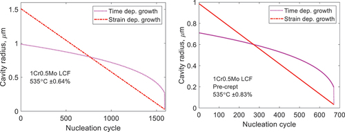
The use of Eqs. (18)(18) $\frac{d{R}_{\mathrm{c}\mathrm{a}\mathrm{v}}}{dt}=2D_0{K}_f(\sigma -{\sigma }_0)\frac{1}{{R_{\mathrm{c}\mathrm{a}\mathrm{v}}}^2}$(18) and (19(19) $R_{\mathrm{c}\mathrm{a}\mathrm{v}}=C_{\mathrm{s}}\epsilon$(19) ) is illustrated in Figure 9 for two cases in Table 1 for the 1Cr0.5Mo steel. During the growth process, a distribution of cavity sizes is obtained. In Figure 9, the cavity size is given a function of the cycle it was nucleated in. Cavities that are nucleated at an early stage can grow more than those nucleating at a later stage. Strain controlled growth gives a linear dependence in Figure 9 whereas diffusion controlled is occurring at a higher speed initially but slows down gradually. The two types of growth give about the same cavity sizes. Detailed measurements of the cavity size were not carried out in [23]. It would not have been simple anyway because the specimens were etched. Considering this, the predicted cavity sizes are of the right order in comparison to the micrographs.

Figure 9. Cavity radius versus the cycle where the cavity was nucleated. Two examples from the tests in Table 1 for 1Cr0.5Mo steel are given the two subfigures. Model values for diffusion controlled growth according to Eq. (18)(18) $\frac{d{R}_{\mathrm{c}\mathrm{a}\mathrm{v}}}{dt}=2D_0{K}_f(\sigma -{\sigma }_0)\frac{1}{{R_{\mathrm{c}\mathrm{a}\mathrm{v}}}^2}$(18) and strain controlled growth, Eq. (19)(19) $R_{\mathrm{c}\mathrm{a}\mathrm{v}}=C_{\mathrm{s}}\epsilon$(19) .

For constrained growth the results for diffusion and strain controlled growth should definitely not be added since each process gives the maximum possible growth rate. For unconstrained growth, this conclusion is not quite so simple to draw. However, if the two growth processes are added in the modelling, the result is a cavity size of about 10 µm, which is not in accordance with the observations. Thus, the two processes should not be added.

Cavity closure

Putting $\sigma$= $\sigma$₀ in Eq. (18)(18) $\frac{d{R}_{\mathrm{c}\mathrm{a}\mathrm{v}}}{dt}=2D_0{K}_f(\sigma -{\sigma }_0)\frac{1}{{R_{\mathrm{c}\mathrm{a}\mathrm{v}}}^2}$(18) gives the minimum cavity radius R_cavmin (cavity nucleus)

(20) $R_{\mathrm{c}\mathrm{a}\mathrm{v}\mathrm{m}\mathrm{i}\mathrm{n}}=2{\gamma }_{s}sin(\alpha )/\sigma$(20)

R_cavmin is about 1.5 × 10⁻² µm for the 1Cr0.5Mo steel. It has been verified experimentally that the value in Eq. (20)(20) $R_{\mathrm{c}\mathrm{a}\mathrm{v}\mathrm{m}\mathrm{i}\mathrm{n}}=2{\gamma }_{s}sin(\alpha )/\sigma$(20) is close to the observed nucleus size for copper. This has been shown with the help of small-angle neutron scattering [25].

With the help of Eq. (18)(18) $\frac{d{R}_{\mathrm{c}\mathrm{a}\mathrm{v}}}{dt}=2D_0{K}_f(\sigma -{\sigma }_0)\frac{1}{{R_{\mathrm{c}\mathrm{a}\mathrm{v}}}^2}$(18) it ought to be possible to estimate the number of cavities that are closed during compression going part of the cycle. No formation of new cavities during the compression part of the cycles is assumed. The direct application of Eq. (18)(18) $\frac{d{R}_{\mathrm{c}\mathrm{a}\mathrm{v}}}{dt}=2D_0{K}_f(\sigma -{\sigma }_0)\frac{1}{{R_{\mathrm{c}\mathrm{a}\mathrm{v}}}^2}$(18) to estimate the closure does not work. This can be seen in the following way. According to Eq. (19)(19) $R_{\mathrm{c}\mathrm{a}\mathrm{v}}=C_{\mathrm{s}}\epsilon$(19) a cavity with a size of about 1 × 10⁻³ µm is formed in each cycle. Applying Eq. (18)(18) $\frac{d{R}_{\mathrm{c}\mathrm{a}\mathrm{v}}}{dt}=2D_0{K}_f(\sigma -{\sigma }_0)\frac{1}{{R_{\mathrm{c}\mathrm{a}\mathrm{v}}}^2}$(18) to this nucleus would make it disappear within fractions of a second. Thus, no cavities would be formed and this is not in agreement with the observations. Instead, it has to be assumed that a cavity is created first after a number of load cycles.

The strain rate in the LCF tests for 1Cr0.5Mo was 0.003/s, which means that the compression part of the cycle takes 3 s. During this time, cavities that are smaller than R_cavmin/2.5 are dissolved. With initial cavity sizes in the range 0 to 2 R_cavmin, about 20% of the cavities would be closed. Thus, the constant f_close in Eq. (17)(17) $n_{cav}=B_{\mathrm{s}}(1-f_{\mathrm{c}\mathrm{l}\mathrm{o}\mathrm{s}\mathrm{e}})(\mathrm{\Delta }{\epsilon }_{\mathrm{h}\mathrm{o}\mathrm{l}\mathrm{d}}+\mathrm{\Delta }{\epsilon }_{\mathrm{c}\mathrm{r}\mathrm{\_}\mathrm{t}\mathrm{e}\mathrm{n}\mathrm{s}}+\mathrm{\Delta }{\epsilon }_{\mathrm{c}\mathrm{r}\mathrm{\_}\mathrm{c}\mathrm{m}\mathrm{p}\mathrm{r}})N_{\mathrm{c}\mathrm{y}\mathrm{c}\mathrm{l}}$(17) would be 0.2. However, this value is uncertain, and it has not been taken into account when calculating the number of cavities in Figures 7 and 8.

The model for the hysteresis loop has been demonstrated to be valid for an austenitic stainless steel, for 1Cr0.5Mo steel and for an oxide dispersion strengthened ferritic steel [6]. The model can therefore be considered to have general applicability. The derivation of the models for the number of cavities and cavity growth are general and based on physical principles, and they should be possible to use in different applications. However, the cavitation data during LCF for the 1Cr0.5Mo steel are almost unique, and consequently, it has only been possible to verify the models against this material. Comparison to data for other materials would be of interest.

Conclusions

• The assessment of creep damage with the help of cavitation is quite useful. This situation has been further improved in recent years by the development of quantitative models for cavity nucleation. Cavitation during cyclic loading is expected to be of the same importance as for static loading. In spite of this, only a limited amount of quantitative cavitation data are available in the literature. In the present paper, previously published cavitation data for a ferritic-bainitic 1Cr0.5Mo steel during LCF at 535ºC are analysed.

• A recently published model for hysteresis loops has been applied. After a creep model has been formulated, the LCF hysteresis loops for 1Cr0.5Mo could be modelled. The influence of pre-creep and hold time in the cycles could successfully be described.

• A model that is well documented for the prediction of the number of cavities during creep was applied. With the help of the model for the stress-strain loops, the creep strain in the load cycle could be determined. It is mainly due to the creep strain during the hold time. By multiplying by the number of cycles, the total creep strain can be obtained. This value was used in the cavitation model. The number of cavities could be reproduced after pre-creep, and after LCF in the tempered condition as well as after pre-creep.

• Both diffusion- and strain-controlled cavity growth has been analysed. The creep strain during the load cycles is quite small. It is quite unlikely that an equilibrium between the growth rate and the creep rate is established and the growth is therefore assumed to be unconstrained. In the strain controlled model, the cavity size is considered to be the same as the amount of grain boundary sliding. The two mechanisms give about the same cavity growth for the 1Cr0.5Mo steel. The mechanisms should not be added because that gives cavity sizes far larger than in the observations.

• It is expected that some cavities are closed during the compression part of a load cycle. In principle, the amount of closure should be possible to predict from the expression for unconstrained growth. According to this formula, sufficiently small cavities should shrink rather than grow. However, it has to be assumed that cavitation takes place stepwise and first after a number of load cycles. Although such an assumption is feasible, it has to be verified experimentally. The amount of cavity closure during LCF remains an open issue.

Disclosure statement

No potential conflict of interest was reported by the author.

Additional information

Funding

The work was supported by the Swedish Nuclear Fuel and Waste Management Co (SKB) [4501751122].

References

- Lundberg L, Sandstrom R. Application of low cycle fatigue data to thermal fatigue cracking. Scand J Metall. 1982;11:85–104.
- Arrell D, Hasselqvist M, Sommer C, et al., On TMF damage, degradation effects, and the associated TMin influence on TMF test results in γ/γ′ alloys, in Proceedings of the International Symposium on Superalloys, 2004, pp. 291–294.
- Miller DA, Priest RH, Ellison EG. Review of material response and life prediction techniques under fatigue-creep loading conditions. High Temp Mater Process. 1984;6:155–194.
- Sandström R, He J. Survey of creep cavitation in fcc metals. Study of Grain Boundary Character. 2017.
- Holdsworth SR. Creep-fatigue properties of high temperature turbine steels. Mater High Temp. 2001;18:261–265.
- Sandström R. Basic creep-fatigue models considering cavitation. Transactions of the Indian National Academy of Engineering. 2022;7:583–591.
- Lim LC. Cavity nucleation at high temperatures involving pile-ups of grain boundary dislocations. Acta Metall. 1987;35:1663–1673.
- Crossman FW, Ashby MF. The non-uniform flow of polycrystals by grain-boundary sliding accommodated by power-law creep. Acta Metall. 1975;23:425–440.
- McLean D, Farmer MH. The relation during creep between grain-boundary sliding, sub-crystal size, and extension. J Inst Met. 1957;85:41–50.
- Sandström R, Wu R. Influence of phosphorus on the creep ductility of copper. J Nucl Mater. 2013;441:364–371.
- He J, Sandström R. Formation of creep cavities in austenitic stainless steels. J Mater Sci. 2016;51:6674–6685.
- Beere W, Speight MV. Creep cavitation by vacancy diffusion in plastically deforming solid. Met Sci. 1978;21:172–176.
- Dyson BF. Constraints on diffusional cavity growth rates. Met Sci. 1976;10:349–353.
- Rice JR. Constraints on the diffusive cavitation of isolated grain boundary facets in creeping polycrystals. Acta Metall. 1981;29:675–681.
- He J, Sandström R. Creep cavity growth models for austenitic stainless steels. Materials Science & Engineering A. 2016;674:328–334.
- Sandström R, He J-J. Prediction of creep ductility for austenitic stainless steels and copper. Mater High Temp. 2022; 39:1–9.
- He J, Sandström R. Basic modelling of creep rupture in austenitic stainless steels. Theor Appl Fract Mech. 2017;89:139–146.
- Sandström R, Fundamental models for the creep of metals, in Creep, inTech, 2017.
- Sandström R, Hallgren J. The role of creep in stress strain curves for copper. J Nucl Mater. 2012;422:51–57.
- Sandstrom R. Basic model for primary and secondary creep in copper. Acta Mater. 2012;60:314–322.
- Andersson HCM, Sandstrom R, Debord D. Low cycle fatigue of four stainless steels in 20% CO-80% H-2. Int J Fatigue. 2007;29:119–127.
- Data sheets on the elevated-temperature properties of normalized and tempered 1cr-0.5mo steel plates for pressure vessels (SCMT 2 NT). Tokyo, Japan: National Research Institute for Metals; 2002.
- Storesund J, Sandstrom R. Interaction of creep damage and low cycle fatigue damage in a 1Cr0.5Mo steel. ISIJ Int. 1990;30:875–884.
- Ghahremani F. Effect of grain boundary sliding on steady creep of polycrystals. Int J Solids Struct. 1980;16:847–862.
- Das Y, Fernandez-Caballero A, Elmukashfi E, et al. Stress driven creep deformation and cavitation damage in pure copper. Materials Science & Engineering A. 2021;833:142543.