Estimating the Monkman−Grant relation in the presence of errors in measurement of times to failure and minimum creep rates: with application to some high temperature materials

ABSTRACT

The Monkman−Grant relation has the potential to reduce the development cycle for new materials, as it provides a means of lifting based on minimum creep rates that are typically observed early on. This paper outlines problems in estimating the nature of this relation using the least squares technique that stems from errors made in measuring failure times and minimum creep rates. The paper outlines some solutions to this problem that have been proposed within the scientific literature – such as reverse regression and the Deming regression. The evidence from the materials studied in this paper, suggest that the use of least squares results in overly conservative lifetime predictions when using the Monkman-Grant relation. It was found that for 2.25Cr-1Mo steel, the life expected for a minimum creep rate of 3.67E-12s⁻¹ was 57 years when the least squares technique was used, but this increased to 78 years when using the Deming regression.

KEYWORDS:

• Monkman-Grant relation
• measurement errors
• least squares
• total least squares
• Deming regression

Introduction

For materials operating at high temperatures, the understanding of creep and its interaction with other damage mechanism such as fatigue and oxidation are of great importance. Indeed, creep is the dominant failure mechanism for pipework that is used to transport steam from boilers to turbines in power plants. Currently, expensive testing programmes lasting 12–15 years are required to determine the long-term strengths and lives. A reduction in this ‘materials development cycle’ was therefore defined as the No.1 priority in the 2007 UK Energy Materials – Strategic Research [1]. For materials where the Monkman−Grant [2] relation is stable over time, a lifetime prediction can be made using measured minimum creep rates. As the minimum creep rate is reached well before rupture, this approach also offers the potential to reduce the length and cost of these testing programmes. When using this approach, the unknown parameters of the Monkman−Grant relation are typically estimated from a direct application of the least squares technique to data collected on time to failure and minimum creep rates. But as this paper illustrates, this approach will produce reliable estimates only when the minimum creep rate is measured without error.

In practice, the variables measured during creep are all subject to measurement error. For example, Foster [3] in an SM&T Project paper (No. SMT4-CT97-2165) concluded that when measuring creep failure time, the major sources of error in its measurement were due to limitations in controlling the ambient temperature, errors in measuring stress (in a constant stress test) and the data logger time interval. Minor contributions to the measurement error associated with failure times include errors in measuring load (in a constant load creep test), the initial dimensions of the specimen and specimen temperature. All the above sources also contribute to the errors in measuring the minimum creep rate, with additional major contributions stemming from measurement errors associated with the extensometer, errors in measuring the time to minimum creep rate and errors associated with the graphical or statistical methods used to identify the minimum slope from the experimental creep curve (for example the standard errors of the theta parameters used to describe a creep curve using the theta methodology and the scatter around such a fitted curve [4]).

The error in measuring the creep load is derived from the calibration certificate of the load cell or lever system and weights. Assuming a rectangular distribution, the standard uncertainty in this load is given by ± s/√3, where ±s is the certified maximum error. Temperature (T) uncertainty is found by combining the maximum errors made by the thermocouple em(T), errors made in measuring the along-specimen uniformity eu(T) and the errors made by the measuring system itself ec(T) – all of which change with the magnitude of temperature. The standard uncertainty in temperature is then

$\surd \left[\left(\mathrm{em}{\left(\mathrm{T}\right)}^2+\mathit{\hspace{0.17em}}\mathrm{eu}{\left(\mathrm{T}\right)}^2+\mathit{\hspace{0.17em}}\mathrm{ec}{\left(\mathrm{T}\right)}^2\right)\right]\mathit{\hspace{0.17em}}/\surd 3$

Uncertainty in measuring the time to failure t_F is due to the length of the data logging time period ∆t – or ∆t/(2√3) assuming a rectangular distribution. This uncertainty also depends on the errors in measuring stress and the errors in measuring temperature. The contribution of these last two errors to the error in measuring t_F is determined by the values for Norton’s n and the activation energy Q_c. Similarly, n and Q_c will determine the contribution of stress and temperature error measurements to errors in the measurement of the minimum creep rate. These can then be combined with the statistical methods errors described above.

Foster [3] found in his study on 2.25Cr-1Mo weld metal at 565 °C, the thermocouple error was around 2 °C, the specimen uniformity error around 1.5 °C and the measuring system error around 2 °C. The error in measuring the load was ± 1%. At 565 °C and 170 MPa, the measurement errors on t_F were ± 1482 h (with 2.3 h of this due to the data logging time, 71 h due to errors in measuring stress and the rest due to temperature measurement errors). At the same test condition, the measurement error on the minimum creep rate was estimated at ±2.2E-6 h⁻¹ (with 3.1E-07 h⁻¹ of this due to stress measurement errors and the rest due to temperature errors). That due to statistical methods was not quantified, so the overall measurement error is likely to be much higher.

Therefore, this paper aims to review the statistical literature on errors in variables to bring to the attention of the materials research community, how and in what ways the direct application of least squares to the Monkman−Grant relation produces unreliable parameter estimates. It then presents some solutions to this problem. Finally, the paper applies these solutions to several different materials to assess the severity of the parameter unreliability in the face of measurement errors. To achieve these aims, the paper is structured as follows. The next section summarises the three data sets used to illustrate the consequences of measurement error. The method section then describes the desirable properties of the least squares estimators, how measurement errors lead to a breakdown of these properties, and what solutions to this issue exist. The results section applies the reviewed alternative estimation techniques to data on a low Chrome Steel, a Nickel based super alloy and a 403-B Stainless Steel. Suggestions for future research are given in the conclusions section.

The data

This paper makes use of the information in Creep Data Sheets 3B, 15B, 34B published by the Japanese National Institute for Materials Science (NIMS) [5–7]. Data sheet 3B has extensive data on 12 batches of 2.25Cr-1Mo (according to ASTM A 387, Grade 22) steel where each batch has a different chemical composition that underwent one of four different heat treatments – details of which are given in [5]. This paper makes use of just one of these batches, the MAF batch, which was in tube form that had an outside diameter of 50.8 mm, a wall thickness of 8 mm and a length of 5000 mm with a chemical composition of: Fe − 2.46 Cr − 0.94 Mo − 0.1 C − 0.23 Si − 0.43 Mn − 0.011 P − 0.009 S − 0.043 Ni − 0.07 Cu − 0.005 Al. Specimens for creep testing were taken longitudinally from this material. Each test specimen had a diameter of 6 mm with a gauge length of 30 mm. The creep tests were obtained over a wide range of test conditions: 333−22 MPa and 723−923 K. The MAF batch was the only one for which both failure times and minimum creep rate measurements were made.

Data sheet 15B has extensive data on 6 batches of 18Cr-12Ni-Mo Stainless Steel bars where each batch has a different chemical composition that underwent one of three different heat treatments – details of which are given in [6]. This paper makes use of all these batches, which were in bar form. Specimens for creep testing were taken longitudinally from these square bars. The test specimens had a diameter of 10 mm in diameter and a gauge length of 50 mm. The creep tests were conducted over a wide range of test conditions: 265−20 MPa and 873−1073K.

Data sheet 34B has extensive data on 6 batches of Nickel based 19Cr-18Co-4Mo-3Ti super alloy castings that underwent one of three different heat treatments. It also had 3 batches of Nickel based 19Cr-18Co-4Mo-3Ti super alloy forgings that underwent one of three different heat treatments. Each batch had a different chemical composition – details of which are given in [7]. As both failure times and minimum creep rates were recorded for only the forged material, only forgings are used in this paper. Specimens for creep testing were taken longitudinally from round bars. The test specimens had a geometry with 6 mm in diameter and a 30 mm gauge length. The creep tests were conduced over a wide range of conditions: 235−24 MPa and 1073−1273K.

Methodology

Properties of least squares estimators in the absence of measurement errors

The properties of least squares estimates are now discussed with reference to the Monkman−Grant [2] relation. Let t_Fi be the measured time to failure at test condition i and ${\dot{\epsilon }}_{\mathrm{mi}}$, the corresponding measured minimum creep rate at this condition. Suppose also that the creep test matrix is made up of some n such test conditions, some of which may be repeats. The Monkman−Grant [2] relation can then be written as

(1a) ${\mathrm{t}}_{\mathrm{Fi}}=\mathrm{M}{\dot{\epsilon }}_{\mathrm{mi}}^{\mathit{\rho }}\mathrm{or}\mathit{\hspace{0.17em}}{\mathrm{Y}}_{\mathrm{i}}=ln[\mathrm{M}]+\mathit{\rho }{X}_{\mathrm{i}}$(1a)

where Y_i = ln[t_Fi] and X_i = ln[${\dot{\epsilon }}_{\mathrm{mi}}]$. For the moment it is assumed that these two variables are measured without error so that Y and X represent their true values. Tests specimens will typically be cut from different positions within the supplied bar, tube or plate for a particular material and consequently the specimens will all have slightly different characteristics such as grain size, number of inclusions and other microstructural characteristics (all leading to them having different degrees of hardness). In bigger data sets, the specimens will all have experienced different heat treatments and will have different chemical compositions – but all within the specifications/standards defining a particular grade of material. The result is that each specimen will have a life that is slightly different to that expected from its minimum creep rate, that is, slightly different to that given by Equation (1a)(1a) ${\mathrm{t}}_{\mathrm{Fi}}=\mathrm{M}{\dot{\epsilon }}_{\mathrm{mi}}^{\mathit{\rho }}\mathrm{or}\mathit{\hspace{0.17em}}{\mathrm{Y}}_{\mathrm{i}}=ln[\mathrm{M}]+\mathit{\rho }{X}_{\mathrm{i}}$(1a) . This phenomenon is captured through the addition of an omission error term (e_i) to Equation (1a)(1a) ${\mathrm{t}}_{\mathrm{Fi}}=\mathrm{M}{\dot{\epsilon }}_{\mathrm{mi}}^{\mathit{\rho }}\mathrm{or}\mathit{\hspace{0.17em}}{\mathrm{Y}}_{\mathrm{i}}=ln[\mathrm{M}]+\mathit{\rho }{X}_{\mathrm{i}}$(1a)

(1b) ${\mathrm{Y}}_{\mathrm{i}}=ln\left[\mathrm{M}\right]+\mathit{\rho }{\mathrm{X}}_{\mathrm{i}}+{\mathrm{e}}_{\mathrm{i}}$(1b)

This error of omission is interpreted as picking up the above-mentioned omitted variables from the model. For example, the time at which a specimen fails will not just depend on its minimum creep rate (which in turn is determined by the stress and temperature the specimen is placed on test at), but also on other variables such as the specimen’s chemical composition (within the materials grade specification), the heat treatment, grain size and other microstructural characteristics. e_i may also contain errors in measuring Y without altering any of the desirable properties identified next.

The Monkman–Grant relation has been estimated for many materials, and in most of these instances the unknown parameters M and ρ were estimated by direct application of the least squares technique under the assumption of zero measurement errors on variable X. This technique aims to minimises $\sum _{\mathrm{i}=1}^{\mathrm{n}}{e}_i^2$. The solution to this minimisation takes the form

(2) $\text{{}\widehat{\text{M}}=\text{exp}[\overline{\text{Y}}-\widehat{\text{p}}\overline{\text{X}}]\text{with}\widehat{\text{p}}\text{=}\sum \text{i=1n }({\text{Y}}_{\text{i}}\text{-}\overline{\text{Y}})({\text{X}}_{\text{i}}\text{-}\overline{\text{X}}){\displaystyle {\sum }_{\text{i=1}}^{\text{n}}{({\text{X}}_{\text{i}}\text{-}\overline{\text{X}})}^{\text{2}}}$(2)

where the hat symbol indicates that these are least squares estimates of the parameters M and ρ made from the given sample of data (capitals are used for variable names because it is assumed there are no measurement errors). These least squares estimators are termed linear estimators as the parameters are linear combinations of all the values for Y_i – for example, $\widehat{\rho }={\displaystyle {\sum }_{\mathit{i}=1}^n{k}_i}{\text{(Y}}_{\text{i}}-\overline{\text{Y}}\text{)}$ where $\mathrm{ki}=\mathit{\hspace{0.17em}}\frac{\left({\mathrm{X}}_i-\bar{\mathrm{X}}\right)}{{\sum }_{\mathrm{i}=1}^{\mathrm{n}}{\left({\mathrm{X}}_i\mathit{\hspace{0.17em}}-\bar{\mathrm{X}}\right)}^2}$.

If the mean value for all the e_i is zero, and if the e_i are independent of X_i, then $\hat{M}$ and $\hat{\rho }$ will be unbiased (see Appendix A for proof). Further, if the e_i have constant variance and are also independent of each other, then $\hat{M}$ and $\hat{\rho }$ will also be efficient (see Appendix A). Unbiasedness and efficiency are small sample properties.

These terms can be understood in terms of hypothetical repeated random sampling. In this sampling process, all possible samples of size n that are made up of observations on Y_i and X_i are taken (i.e. an infinite number of such samples are collected), and for each sample the estimates $\hat{M}$ and $\hat{\rho }$ are computed using Equation (2)(2) $\text{{}\widehat{\text{M}}=\text{exp}[\overline{\text{Y}}-\widehat{\text{p}}\overline{\text{X}}]\text{with}\widehat{\text{p}}\text{=}\sum \text{i=1n }({\text{Y}}_{\text{i}}\text{-}\overline{\text{Y}})({\text{X}}_{\text{i}}\text{-}\overline{\text{X}}){\displaystyle {\sum }_{\text{i=1}}^{\text{n}}{({\text{X}}_{\text{i}}\text{-}\overline{\text{X}})}^{\text{2}}}$(2) , so that many estimates for each of these parameters would be obtained. If the mean (called the expected value or E for short) of all these values equals the true (i.e. population) value, then the estimate is said to be unbiased. Unbiasedness therefore requires E($\hat{M})=\mathit{M}$ and $\mathit{E}\left(\hat{\rho }\right)=\mathit{\rho }$ (E is the expectations operator). Appendix A proves that if the mean value for e_i equals zero and if e_i and x_i are independent of each other, then the least squares estimate of ρ and ln(M) are unbiased.

The variance in all these least squares estimates for M and ρ are given by

(3) $\text{Var}\left(\text{ln}(\widehat{\text{M}})\right)=\frac{{\sigma }_{\text{e}}^2{\displaystyle {\sum }_{\text{i}=1}^{\text{n}}{\text{Y}}_{\text{i}}^2}}{\text{n}{\displaystyle {\sum }_{\text{i}=1}^{\text{n}}{\left({\text{X}}_{\text{i}}-\overline{\text{X}}\right)}^2}}=\sum \text{\_i}=1\text{^n\_}{\widehat{{\text{e}}_{\text{i}}}}^2{\displaystyle {\sum }_{\text{i}=1}^{\text{n}}{\text{Y}}_{\text{i}}^2}\left(\text{n}-2\right)\text{n}{\displaystyle {\sum }_{\text{i}=1}^{\text{n}}{\left({\text{X}}_{\text{i}}-\overline{\text{X}}\right)}^2}\text{Var}(\widehat{\text{p}})=\frac{{\sigma }_{\text{e}}^2}{{\displaystyle {\sum }_{\text{i}=1}^{\text{n}}{\left({\text{X}}_{\text{i}}-\overline{\text{X}}\right)}^2}}=\sum \text{i}=1\text{n}{\widehat{{\text{e}}_{\text{i}}}}^2\left(\text{n}-2\right){\displaystyle {\sum }_{\text{i}=1}^{\text{n}}{\left({\text{X}}_{\text{i}}-\overline{\text{X}}\right)}^2}$(3)

where ${\hat{e}}_{\mathit{i}}=Y_i-\left[\hat{M}+\hat{\rho }{X}_i\right]$ and ${\mathit{\sigma }}_{\mathrm{e}}^2$ is the population variance for e which is estimated using the average value for ${\hat{\mathrm{e}}}_{\mathrm{i}}^2$ (adjusting for the 2 degrees of freedom lost in estimating M and ρ).

If all possible samples of size n made up of observations on Y_i and X_i are taken, and for each sample the variance in the estimates of $\hat{M}$ and $\hat{p}$ are computed using Equation (3)(3) $\text{Var}\left(\text{ln}(\widehat{\text{M}})\right)=\frac{{\sigma }_{\text{e}}^2{\displaystyle {\sum }_{\text{i}=1}^{\text{n}}{\text{Y}}_{\text{i}}^2}}{\text{n}{\displaystyle {\sum }_{\text{i}=1}^{\text{n}}{\left({\text{X}}_{\text{i}}-\overline{\text{X}}\right)}^2}}=\sum \text{\_i}=1\text{^n\_}{\widehat{{\text{e}}_{\text{i}}}}^2{\displaystyle {\sum }_{\text{i}=1}^{\text{n}}{\text{Y}}_{\text{i}}^2}\left(\text{n}-2\right)\text{n}{\displaystyle {\sum }_{\text{i}=1}^{\text{n}}{\left({\text{X}}_{\text{i}}-\overline{\text{X}}\right)}^2}\text{Var}(\widehat{\text{p}})=\frac{{\sigma }_{\text{e}}^2}{{\displaystyle {\sum }_{\text{i}=1}^{\text{n}}{\left({\text{X}}_{\text{i}}-\overline{\text{X}}\right)}^2}}=\sum \text{i}=1\text{n}{\widehat{{\text{e}}_{\text{i}}}}^2\left(\text{n}-2\right){\displaystyle {\sum }_{\text{i}=1}^{\text{n}}{\left({\text{X}}_{\text{i}}-\overline{\text{X}}\right)}^2}$(3) , then this estimator is said to be efficient if it is both unbiased and it has the smallest average variance amongst all other possible linear estimators. That is, E[$\hat{M}-\mathit{E}\left(\hat{M}\right)$]² < E[$\stackrel{⌣}{M}-\mathit{E}(\stackrel{⌣}{M}$]² and E[$\hat{\rho }-\mathit{E}\left(\hat{\rho }\right)$]² < E[$\stackrel{⌣}{p}-\mathit{E}(\stackrel{⌣}{p})$]², where the upside down hat signifies any other unbiased linear estimator. Appendix A shows that under the assumption that all the e_i are independent of each other and that the variance of e_i is constant, then the least squares estimate of ρ and M also have minimum variance and so are efficient estimates. So under all the mentioned assumptions, the estimated values for M and ρ from a researchers sample could differ from the true values – but on average they won’t – and further, the chances of them being different from their true values is as small as it possibly can be because the variance is minimised. This is true no matter how small the sample size is.

Consistency is a large sample property and describes what happens to the estimator when it is calculated from a larger and larger sample of data. An estimator is consistent if as the sample size increases the probability of the estimator differing from its true value gets smaller, and in the limit, becomes zero. Assuming independence between e_i and X_i, that the mean of e_i is zero, and that e_i is independent of X_i, Appendix B proves the least squares estimators are consistent estimators. What all this means is that as researchers work with larger and larger samples, the probability of their least squares estimators of $\hat{M}$ and $\hat{\rho }$ differing from the true values M and ρ, tends to zero. It is these properties of unbiasedness, efficiency and consistency that makes the ordinary least squares technique so popular amongst practitioners.

Representing measurement errors statistically

Unfortunately, these desirable properties of the least squares estimator disappear when the variable X is measured with error – which is the realistic situation when it comes to creep testing. This can be demonstrated as follows. On top of these omission errors, there are potentially the errors in measuring X and Y. Let these errors be represented by the variables u_i and v, respectively.

(4a) ${\mathrm{y}}_{\mathrm{i}}=\mathit{\hspace{0.17em}}{\mathrm{Y}}_{\mathrm{i}}+\mathit{\hspace{0.17em}}{\mathrm{u}}_{\mathrm{i}}$(4a)

(4b) ${\mathrm{x}}_{\mathrm{i}}=\mathit{\hspace{0.17em}}{\mathrm{X}}_{\mathrm{i}}+\mathit{\hspace{0.17em}}{\mathrm{v}}_{\mathrm{i}}$(4b)

where y_i is the measured value for ln(t_F) for specimen i and so u_i is the error made in measuring ln(t_F) for this specimen. x_i is the measured value for $ln\left({\dot{\epsilon }}_{\mathit{m}}\right)$ and so v_i is the error made in measuring $ln\left({\dot{\epsilon }}_{\mathit{m}}\right)$ for this specimen. In reality, only y and x are observed in any collected sample of data. The sample moments are therefore given by:

1st order sample moments are denoted by:

(5a) $\bar{x}=\frac{{\sum }_{\mathrm{i}=1}^{\mathrm{n}}{\mathrm{x}}_{\mathrm{i}}}{\mathrm{n}}\mathrm{and}\bar{\mathrm{y}}=\frac{{\sum }_{\mathrm{i}=1}^{\mathrm{n}}{\mathrm{y}}_{\mathrm{i}}}{\mathrm{n}}$(5a)

2nd order moments are denoted by:

(5b) ${\mathrm{s}}_{\mathrm{xx}}=\frac{{\sum }_{\mathrm{i}=1}^{\mathrm{n}}{\left({\mathrm{x}}_{\mathrm{i}}-\bar{\mathrm{x}}\right)}^2}{\mathrm{n}},s_{\mathrm{yy}}=\frac{{\sum }_{\mathit{i}=1}^n{\left({\mathrm{y}}_{\mathrm{i}}-\bar{\mathrm{y}}\right)}^2}{\mathit{n}}\mathrm{and}\text{break}{\mathrm{s}}_{\mathrm{xy}}=\frac{{\sum }_{\mathrm{i}=1}^{\mathrm{n}}\left({\mathrm{x}}_{\mathrm{i}}-\bar{\mathrm{x}}\right)\left({\mathrm{y}}_{\mathrm{i}}-\bar{\mathrm{y}}\right)}{\mathrm{n}}$(5b)

Provided that variables x and y follow a skewed distribution there are also some important 3rd order moments that can be quantified

(5c) ${\mathrm{s}}_{\mathrm{xxy}}=\frac{{\sum }_{\mathrm{i}=1}^{\mathrm{n}}{\left({\mathrm{x}}_{\mathrm{i}}-\bar{\mathrm{x}}\right)}^2\left({\mathrm{y}}_{\mathrm{i}}-\bar{\mathrm{y}}\right)}{\mathrm{n}}\mathrm{and}\text{break}{\mathrm{s}}_{\mathrm{yyx}}=\frac{{\sum }_{\mathrm{i}=1}^{\mathrm{n}}{\left({\mathrm{y}}_{\mathrm{i}}-\bar{\mathrm{y}}\right)}^2\left({\mathrm{x}}_{\mathrm{i}}-\bar{\mathrm{x}}\right)}{\mathrm{n}}$(5c)

but these do require a substantial sample size to quantify reliably (~50+).

The Monkman–Grant model states that the relationship between the true variables Y_i and X_i is given by Equation (1b)(1b) ${\mathrm{Y}}_{\mathrm{i}}=ln\left[\mathrm{M}\right]+\mathit{\rho }{\mathrm{X}}_{\mathrm{i}}+{\mathrm{e}}_{\mathrm{i}}$(1b) . Substituting Equations (4) into Equation (1b)(1b) ${\mathrm{Y}}_{\mathrm{i}}=ln\left[\mathrm{M}\right]+\mathit{\rho }{\mathrm{X}}_{\mathrm{i}}+{\mathrm{e}}_{\mathrm{i}}$(1b) gives

(6a) ${\mathrm{y}}_{\mathrm{i}}-{\mathrm{u}}_{\mathrm{i}}=ln\left[\mathrm{M}\right]+\mathit{\rho }\left({\mathrm{x}}_{\mathrm{i}}-{\mathrm{v}}_{\mathrm{i}}\right)+{\mathrm{e}}_{\mathrm{i}}$(6a)

or

(6b) ${\mathrm{y}}_{\mathrm{i}}=ln\left[\mathrm{M}\right]+\mathit{\rho }{\mathrm{x}}_{\mathrm{i}}+{\mathrm{w}}_{\mathrm{i}}$(6b)

where w_i = $\left({\mathrm{e}}_{\mathrm{i}}+{\mathrm{u}}_{\mathrm{i}}-\mathit{\rho }{\mathrm{v}}_{\mathrm{i}}\right)$. Now notice that an increase in v_i will increase w_i from Equation (6b)(6b) ${\mathrm{y}}_{\mathrm{i}}=ln\left[\mathrm{M}\right]+\mathit{\rho }{\mathrm{x}}_{\mathrm{i}}+{\mathrm{w}}_{\mathrm{i}}$(6b) , but from Equation (4b)(4b) ${\mathrm{x}}_{\mathrm{i}}=\mathit{\hspace{0.17em}}{\mathrm{X}}_{\mathrm{i}}+\mathit{\hspace{0.17em}}{\mathrm{v}}_{\mathrm{i}}$(4b) it will also increase x_i and so w_i and x_i are no longer independent of each other when applying the least squares formulas to Equation (6b)(6b) ${\mathrm{y}}_{\mathrm{i}}=ln\left[\mathrm{M}\right]+\mathit{\rho }{\mathrm{x}}_{\mathrm{i}}+{\mathrm{w}}_{\mathrm{i}}$(6b) . This will result in the values for $\widehat{M}$ and $\widehat{\rho }$ obtained from Equation (2)(2) $\text{{}\widehat{\text{M}}=\text{exp}[\overline{\text{Y}}-\widehat{\text{p}}\overline{\text{X}}]\text{with}\widehat{\text{p}}\text{=}\sum \text{i=1n }({\text{Y}}_{\text{i}}\text{-}\overline{\text{Y}})({\text{X}}_{\text{i}}\text{-}\overline{\text{X}}){\displaystyle {\sum }_{\text{i=1}}^{\text{n}}{({\text{X}}_{\text{i}}\text{-}\overline{\text{X}})}^{\text{2}}}$(2) no longer being unbiased or consistent – they will therefore be biased in both small and large samples – see Appendix C. In Appendix C, the nature of this inconsistency is further revealed to be given by

(7a) $\underset{\mathrm{n}\to \mathrm{\infty }}{\lim }\hat{\rho }=\left[\frac{{\mathit{\rho \sigma }}_{\mathrm{x}}^2+{\mathit{\sigma }}_{\mathrm{x\epsilon }}+{\mathit{\sigma }}_{\mathrm{yv}}+{\mathit{\sigma }}_{\mathit{\epsilon }\mathrm{v}}}{{\mathit{\sigma }}_{\mathrm{x}}^2+2{\mathit{\sigma }}_{\mathrm{xv}}+{\mathit{\sigma }}_{\mathrm{v}}^2)}\right]\ne \mathit{\rho }$(7a)

which does not equal ρ as σ²_x ≠ 0 when X is measured with error. In Equation (7a)(7a) $\underset{\mathrm{n}\to \mathrm{\infty }}{\lim }\hat{\rho }=\left[\frac{{\mathit{\rho \sigma }}_{\mathrm{x}}^2+{\mathit{\sigma }}_{\mathrm{x\epsilon }}+{\mathit{\sigma }}_{\mathrm{yv}}+{\mathit{\sigma }}_{\mathit{\epsilon }\mathrm{v}}}{{\mathit{\sigma }}_{\mathrm{x}}^2+2{\mathit{\sigma }}_{\mathrm{xv}}+{\mathit{\sigma }}_{\mathrm{v}}^2)}\right]\ne \mathit{\rho }$(7a) , ${\mathit{\sigma }}_{\mathrm{x}}^2$ is the population variance for the measured values of X (i.e. of x), ${\mathit{\sigma }}_{\mathrm{v}}^2$ is the population variance of the errors in measuring X, ${\mathit{\sigma }}_{\mathit{\epsilon }\mathrm{v}}$ the population covariance between the errors in measuring X and the combined measurement and omission errors for Y, where ε_i = e_i + u_i. ${\mathit{\sigma }}_{\mathrm{x\epsilon }}$ is the population covariance between x and ε, ${\mathit{\sigma }}_{\mathrm{yv}}$ is the population covariance between y and v and $2{\mathit{\sigma }}_{\mathrm{xv}}$ is twice the population covariance between x and v. Whether the least squares technique produces estimates with an upward or downward bias depends on the relative sizes of all these terms. To explore this further, consider some assumptions for possible simplification:

1. The measurement/omission errors are independent of the true values of these variables, or ${\mathit{\sigma }}_{\mathit{Y\epsilon }}={\mathit{\sigma }}_{\mathrm{xv}}=0$. This seems reasonable, especially as v_i and ε_i represent the size of the errors made in measuring log failure times and log minimum creep rates. So, even if the error in measuring failure times and creep rates does change with their magnitudes (which is likely given the discussion in the introduction on errors in measuring temperature), provided the percentage error is unchanged, ${\mathit{\sigma }}_{\mathrm{y\epsilon }}={\mathit{\sigma }}_{\mathrm{xv}}=0$. This is because ε and v measure percentage errors as they represent the error in measuring the natural logs of failure times and minimum creep rates.

2. The error in measuring ln(t_F) is independent from the true value for ln[${\dot{\epsilon }}_{\mathrm{m}}]$ or ${\mathit{\sigma }}_{\mathrm{x\epsilon }}$ = 0 and the error in measuring ln[${\dot{\epsilon }}_{\mathrm{m}}]$ is independent from the true value for ln(t_F) or ${\mathit{\sigma }}_{\mathrm{yv}}$ = 0. Given the percentage error argument above, this also seems a reasonable assumption.

Under these two reasonable assumptions, Equation (7a)(7a) $\underset{\mathrm{n}\to \mathrm{\infty }}{\lim }\hat{\rho }=\left[\frac{{\mathit{\rho \sigma }}_{\mathrm{x}}^2+{\mathit{\sigma }}_{\mathrm{x\epsilon }}+{\mathit{\sigma }}_{\mathrm{yv}}+{\mathit{\sigma }}_{\mathit{\epsilon }\mathrm{v}}}{{\mathit{\sigma }}_{\mathrm{x}}^2+2{\mathit{\sigma }}_{\mathrm{xv}}+{\mathit{\sigma }}_{\mathrm{v}}^2)}\right]\ne \mathit{\rho }$(7a) simplifies to

(7b) $\underset{\mathrm{n}\to \mathrm{\infty }}{\lim }\hat{\rho }=\left[\frac{{\mathit{\rho \sigma }}_{\mathrm{x}}^2+{\mathit{\sigma }}_{\mathit{\epsilon }\mathrm{v}}}{{(\mathit{\sigma }}_{\mathrm{x}}^2+{\mathit{\sigma }}_{\mathrm{v}}^2)}\right]\ne \mathit{\rho }$(7b)

Equation (7b)(7b) $\underset{\mathrm{n}\to \mathrm{\infty }}{\lim }\hat{\rho }=\left[\frac{{\mathit{\rho \sigma }}_{\mathrm{x}}^2+{\mathit{\sigma }}_{\mathit{\epsilon }\mathrm{v}}}{{(\mathit{\sigma }}_{\mathrm{x}}^2+{\mathit{\sigma }}_{\mathrm{v}}^2)}\right]\ne \mathit{\rho }$(7b) shows that the least squares estimate of ρ will be biased downwards if the measurement errors are positively correlated and if ${\mathit{\sigma }}_{\mathit{\epsilon }\mathrm{v}}$ > ${\mathit{\sigma }}_{\mathrm{v}}^2$. An upward bias occurs when these measurement errors are negatively correlated. Given the most likely scenario is that ${\mathit{\sigma }}_{\mathit{\epsilon }\mathrm{v}}$ >0, as measurement errors for X and Y come from the same sources as discussed in the introduction section, the least squares technique is most likely to produce a downward bias. For further clarity, assume that:

(iii) The measurement errors are unrelated (${\mathit{\sigma }}_{\mathit{\epsilon v}}=0)$. This third assumption may or may not be realistic because as seen in the introduction section, some of the errors in measuring t_F and ${\dot{\epsilon }}_{\mathrm{m}}$ are from the same source – namely errors in measuring stress and temperature. This may result in ε and v being correlated. But this is not guaranteed because each of these variables also have their own unique sources of measurement error. For example, errors stemming from the accuracy of the extensometer will determine the value for v but not ε. Similarly, errors stemming from the measurement of time to various strains will determine the values for v but not for u and the same is true for the errors stemming from statistical and graphical techniques – which given the scatter typical observed in measured strain rates is likely to be a very big source of measurement error. Consequently, assumption iii could well be satisfied in practice, in which case Equation (7b)(7b) $\underset{\mathrm{n}\to \mathrm{\infty }}{\lim }\hat{\rho }=\left[\frac{{\mathit{\rho \sigma }}_{\mathrm{x}}^2+{\mathit{\sigma }}_{\mathit{\epsilon }\mathrm{v}}}{{(\mathit{\sigma }}_{\mathrm{x}}^2+{\mathit{\sigma }}_{\mathrm{v}}^2)}\right]\ne \mathit{\rho }$(7b) would further simplify to

(7c) $\underset{\mathrm{n}\to \mathrm{\infty }}{\lim }\hat{\rho }=\mathit{\rho }\left[\frac{1}{1+{\mathit{\sigma }}_{\mathrm{v}}^2/{\mathit{\sigma }}_{\mathrm{x}}^2)}\right]<\mathit{\rho }$(7c)

Given that $\frac{{\mathit{\sigma }}_{\mathrm{v}}^2}{{\mathit{\sigma }}_{\mathrm{x}}^2}>0$, it follows that under the above three assumptions, $\hat{\rho }$ has a definite downward bias in small and large samples. In what follows let’s further assume that:

• (iv) The measurement errors have a zero mean and a constant variances so that E[ε] = E[v] = 0 and E[ε²] = σ²_ε and E[v²] = σ²_v.

• (v) Both sources of measurement error are serially independent so E[ε_iε_j] = E[v_iv_j] = 0 (for i ≠ j).

Solutions to the presence of measurement errors

Reverse least squares

Reverse least squares [8] involves the regression of x on y

(8a) ${\mathrm{x}}_{\mathrm{i}}=\frac{-ln\left[\mathrm{M}\right]}{\mathit{\rho }}+\frac{1}{\mathit{\rho }}{\mathrm{y}}_{\mathrm{i}}+{\mathrm{w}}_{\mathrm{i}}^{\ast }$(8a)

where ${\mathrm{w}}^{\ast }\mathrm{i}=\mathit{\hspace{0.17em}}({\mathrm{v}}_{\mathrm{i}}-\frac{1}{\mathit{\rho }}\left({\mathrm{e}}_{\mathrm{i}}+{\mathrm{u}}_{\mathrm{i}}\right)$

and this will produce consistent estimates of ρ and M only when variable Y_i is measured without error. If not, an increase in u_i will increase both y_i and w*_i which leads to biased and inconsistent estimates of 1/ρ and thus of ρ. But this time the bias is in the opposite direction to least squares – see Appendix C for proof. Thus, a normal and reverse regression can be used to get upper and lower bounds on ρ – at least in large samples, i.e. to obtain consistent bounds

(8b) ${\left(\underset{\mathrm{n}\to \mathrm{\infty }}{\lim }\hat{\rho }\right)}^{-1}<\mathit{\rho }>\underset{\mathrm{n}\to \mathrm{\infty }}{\lim }\hat{\rho }$(8b)

Total least squares

Total least squares (TLS) or perpendicular least squares [9] is another potential solution to errors in variables. The idea behind TLS is illustrated in Figure 1. The shown line with positive slope shows the true relationship between variables X and Y. That is, if X and Y were both measured without errors all the observed pairings on (y_i, x_i) would fall on this line. The working assumption behind least squares is that the observed pairings are pushed off this line because of errors in omission (e_i) and errors in measuring variable Y (i.e. u_i). X is measured without error so X = x. This is illustrated in scenario 1 of Figure 1, where the circular data point is pushed vertically above the line at X = X₁ by the size of e_i + u_i. The shown distribution encompasses all the possible values that y could take when X = X₁. So, in least squares estimation, we would find the values for ln(M) and ρ that minimise the sum of the squares of the vertical distance between the fitted line and the data. That is, minimising the sum of the squared omission errors plus the squared errors in measuring variable Y.

Figure 1. Visualisation of the various estimation procedures summarised as scenarios 1–4.

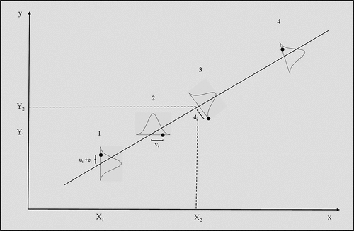
This completely ignores the measurement errors associated with variable X, which leads to a downward bias in the resulting estimate of ρ (and a corresponding upward bias in M). The working assumption behind reverse regression is that the observed pairings are pushed off the true line because of errors in measuring variable X (i.e. v_i). Y is measured without error so Y = y. This is illustrated in scenario 2 of Figure 1, where the circular data point is pushed horizontally to the right of the true line at Y = Y₁ by the size of the error in measuring X, or by v_i. The shown distribution encompasses all the possible values that x could take when Y = Y₁. So in reverse regression, we would find the values for ln(M) and ρ that minimise the sum of the squares of the horizontal distance between the fitted line and the data. That is, minimising the sum of the squared errors in measuring variable X.

Total least squares on the other hand, has the working assumption that the observed data point is pushed off the true line because of errors in measuring X and Y (including omission errors). TLS further assumes that the errors associated with X and Y are equal in value and independent of each other. This is illustrated in scenario 3 of Figure 1, where the circular data point is pushed below the true line because of errors in measuring X and Y. The perpendicular distance d_i is a combination of v_i and e_i + u_i The distribution of (y_i, x_i) pairings seen in scenario 3 encompasses all possible values these observed pairings could take when the true values for X and Y are X = X₂ and Y = Y₂. TLS finds the values for ln(M) and ρ that minimise the sum of the perpendicular distance between the fitted line and the data points. Because the line d_i is perpendicular to the true line, d² = v²+(e + u)² and so TLS places equal weighting on the errors in measuring X and Y when positioning the best fit line.

Scenario 4 places more weighting on the errors in measuring Y when positioning the best fit line. In Figure 2, the light dotted line is positioned to minimise the distance (u_i + e_i)² over all observations. As seen above, this results in too flat a line if there are also errors in measuring variable x_i (if v_i ≠ 0). Reverse regression assumes that deviations in the observed pairings (y_i, x_i) are just the result of errors in measuring x_i (or v_i). Thus, in Figure 2, the solid line is positioned to minimise the distances (v_i)² over all observations. As seen above, this results in too steep a line if there are also omission errors and errors in measuring variable y_i - if u_i + e_i ≠ 0. The scenario in between these two limits is to position a line (the long-dashed line) so as to minimise the square of the perpendicular distance d_i over all observations – so taking into account errors in measuring both y_i and x_i. In Figure 2 the arrowed line d_i is drawn to form a right angle where it intersects the fitted dashed line and so gives the errors u_i + e_i and v_i equal weighting.

Figure 2. The d_i distances used in total least squares illustrated using hypothetical data.

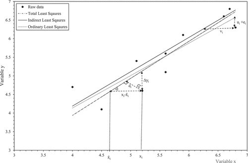
In Figure 2 cosθ = d/Δx or d = cosθΔx. From trigonometric relations, it is known that (1/cos²θ) = sec²θ = 1+ tan²θ. Further, the slope of the fitted dashed line is given by ρ = Δy /$\left({\mathrm{x}}_{\mathrm{i}}-{\hat{\mathrm{x}}}_{\mathrm{i}}\right)$ = tanθ. Consequently, TLS positions the best fit line so as to minimise

(9a) ${\sum }_{\mathrm{i}=1}^{\mathrm{n}}{\mathrm{d}}_{\mathrm{i}}^2=\frac{{\left[{\mathrm{x}}_{\mathrm{i}}-{\hat{\mathrm{x}}}_{\mathrm{i}}\right]}^2}{1+{tan}^2\mathit{\theta }}=\frac{{\left[{\mathrm{x}}_{\mathrm{i}}-{\hat{\mathrm{x}}}_{\mathrm{i}}\right]}^2}{1+{\mathit{\rho }}^2}$(9a)

The solution to this problem has the form

(9b) $\tilde{\rho }=\frac{\mathit{n}{\mathit{s}}_{\mathit{yy}}-\mathit{n}{s}_{\mathit{xx}}+\sqrt{{(\mathit{n}{\mathit{s}}_{\mathit{yy}}-\mathit{n}{s}_{\mathit{xx}})}^2+4\mathit{n}{s}_{\mathit{xy}}^2}}{\frac{}{}}2\mathit{n}{s}_{\mathit{xx}};\text{break}(\tilde{M})=\exp [\bar{y}-\tilde{\rho }\bar{\mathrm{x}}],$(9b)

where the tilde hat denotes a TLS estimator.

The Deming regression

When the errors in measuring X and Y are different in size, this can be accounted for through the addition of a further parameter, λ, with the resulting estimation procedure known as a Deming regression [10]. A Deming regression positions the best fit line so as to minimise

(10a) ${\sum }_{\mathit{i}=1}^n{d}_i^2={\sum }_{\mathit{i}=1}^n\left\{{\left[x_i-{\hat{x}}_{\mathit{i}}\right]}^2+\mathit{\lambda }{\left[y_i-{\hat{y}}_{\mathit{i}}\right]}^2\right\}$(10a)

When λ = 1 this simplifies to the objective function given by Equation (9a)(9a) ${\sum }_{\mathrm{i}=1}^{\mathrm{n}}{\mathrm{d}}_{\mathrm{i}}^2=\frac{{\left[{\mathrm{x}}_{\mathrm{i}}-{\hat{\mathrm{x}}}_{\mathrm{i}}\right]}^2}{1+{tan}^2\mathit{\theta }}=\frac{{\left[{\mathrm{x}}_{\mathrm{i}}-{\hat{\mathrm{x}}}_{\mathrm{i}}\right]}^2}{1+{\mathit{\rho }}^2}$(9a) . The solution to this problem has the form

(10b) $\tilde{\tilde{\rho }}=\frac{\mathit{\lambda n}{\mathit{s}}_{\mathit{yy}}-\mathit{n}{s}_{\mathit{xx}}+\sqrt{{\left(\mathit{\lambda n}{\mathit{s}}_{\mathit{yy}}-\mathit{n}{s}_{\mathit{xx}}\right)}^2+4\mathit{\lambda n}{s}_{\mathit{xy}}^2}}{2\mathit{n\lambda }{s}_{\mathit{xx}}};\text{break}\mathrm{In}\left(\tilde{\tilde{M}}\right)=\exp \left[\bar{y}-\tilde{\tilde{\rho }}\bar{x}\right]$(10b)

and again when λ = 1 this simplifies to Equation (9b)(9b) $\tilde{\rho }=\frac{\mathit{n}{\mathit{s}}_{\mathit{yy}}-\mathit{n}{s}_{\mathit{xx}}+\sqrt{{(\mathit{n}{\mathit{s}}_{\mathit{yy}}-\mathit{n}{s}_{\mathit{xx}})}^2+4\mathit{n}{s}_{\mathit{xy}}^2}}{\frac{}{}}2\mathit{n}{s}_{\mathit{xx}};\text{break}(\tilde{M})=\exp [\bar{y}-\tilde{\rho }\bar{\mathrm{x}}],$(9b) . The double tilde denotes these are Deming estimators. λ measures the relative size of the measurement errors in X and the omission/measurement errors in Y or

(10c) $\mathit{\lambda }=\frac{{\sigma }_{\epsilon }^2}{{\sigma }_v^2}$(10c)

and so the larger is λ, the more weighting is given to the errors associated with y_i when estimating value for M and ρ. In Figure 2, a value for λ different from 1 changes the value for the shown right angle. This technique assumes that λ is a constant over all test conditions and that the measurement errors in x and y are uncorrelated.

Method of moments (MoM)

The Deming regression therefore requires a value for λ before it can be implemented. Often there is a prior or exogenous information on the value for λ (perhaps through repeat testing at the same test conditions), but when this is not the case one possible approach is to combine the method of moments approach with the Deming regression. Provided there is a significant level of skew present in the data on x and y, and ideally that the sample size is at least 50, a reliable Method of Moments estimator of ρ is given by [11]

(11) $\ddot{\rho }={\text{s}}_{\text{yyx}}{\text{s}}_{\text{xxy}}$(11)

where the double dot denotes the MoM estimator for ρ. From the definition of the Pearson correlation coefficient, the population covariance between the true values Y and X equals

(12a) ${\sigma }_{\mathit{YX}}={\rho }^2{{\sigma }^2}_{\mathit{X}}$(12a)

where σ²_X is the population variance for the true value of X. A sample estimate of this covariance is given by $s_{\mathit{xy}}$ and so a sample estimate of σ²_X (or s²_X) is found by also using the method of moments estimator of ρ

(12b) ${\text{s}}^2\text{X}=s_{\mathit{xy}}\ddot{\rho }2$(12b)

From Equation (4b)(4b) ${\mathrm{x}}_{\mathrm{i}}=\mathit{\hspace{0.17em}}{\mathrm{X}}_{\mathrm{i}}+\mathit{\hspace{0.17em}}{\mathrm{v}}_{\mathrm{i}}$(4b) and assumption i above, the population variance for the measured value of x is

(13a) ${\sigma }^2\mathit{x}={{\sigma }^2}_{\mathit{X}}+{\sigma }^2\mathit{v}$(13a)

and a sample estimate of σ²_x is given by s_xx and so a MoM estimate for σ²_v (or s²_v) is given by

(13b) ${{\mathrm{s}}^2}_{\mathit{v}}=\mathit{\hspace{0.17em}}{\mathrm{s}}_{\mathrm{xx}}-\mathit{\hspace{0.17em}}{{\mathrm{s}}^2}_{\mathit{X}}$(13b)

Combining Equation (1b)(1b) ${\mathrm{Y}}_{\mathrm{i}}=ln\left[\mathrm{M}\right]+\mathit{\rho }{\mathrm{X}}_{\mathrm{i}}+{\mathrm{e}}_{\mathrm{i}}$(1b) with Equation (4a)(4a) ${\mathrm{y}}_{\mathrm{i}}=\mathit{\hspace{0.17em}}{\mathrm{Y}}_{\mathrm{i}}+\mathit{\hspace{0.17em}}{\mathrm{u}}_{\mathrm{i}}$(4a) gives

${\mathrm{y}}_{\mathrm{i}}=ln\left[\mathrm{M}\right]+\mathit{\rho }{\mathrm{X}}_{\mathrm{i}}+{\mathrm{e}}_{\mathrm{i}}+u_i=ln\left[\mathrm{M}\right]+\mathit{\rho }{\mathrm{X}}_{\mathrm{i}}+{\mathit{\epsilon }}_{\mathrm{i}}$

where ε_i = e_i + u_i. It follows from this that

(14a) ${\mathit{\sigma }}_{\mathrm{y}}^2={\mathit{\rho }}^2{\mathit{\sigma }}_{\mathrm{X}}^2+{\mathit{\sigma }}_{\mathit{\epsilon }}^2$(14a)

and a sample estimate of ${\mathit{\sigma }}_{\mathrm{y}}^2$ is given by s_yy. Thus, the MoM estimate of σ²_ε (or s²_ε) is given by

(14b) ${\mathrm{s}}_{\epsilon }^2={\mathrm{s}}_{\mathrm{yy}}/({\ddot{\rho }}^2{s^2}_{\mathrm{X}})$(14b)

Consequently, the MoM estimator of λ is

(14c) $\ddot{\lambda }=\frac{{\mathrm{s}}_{\mathit{\epsilon }}^2}{{\mathrm{s}}_{\mathrm{v}}^2}$(14c)

An iterative procedure can then be used, whereby the λ value given by Equation (14c)(14c) $\ddot{\lambda }=\frac{{\mathrm{s}}_{\mathit{\epsilon }}^2}{{\mathrm{s}}_{\mathrm{v}}^2}$(14c) is used in Equation (10b)(10b) $\tilde{\tilde{\rho }}=\frac{\mathit{\lambda n}{\mathit{s}}_{\mathit{yy}}-\mathit{n}{s}_{\mathit{xx}}+\sqrt{{\left(\mathit{\lambda n}{\mathit{s}}_{\mathit{yy}}-\mathit{n}{s}_{\mathit{xx}}\right)}^2+4\mathit{\lambda n}{s}_{\mathit{xy}}^2}}{2\mathit{n\lambda }{s}_{\mathit{xx}}};\text{break}\mathrm{In}\left(\tilde{\tilde{M}}\right)=\exp \left[\bar{y}-\tilde{\tilde{\rho }}\bar{x}\right]$(10b) to update the estimate for ρ to $\tilde{\tilde{\rho }}$. If this value is used in Equations (12b(12b) ${\text{s}}^2\text{X}=s_{\mathit{xy}}\ddot{\rho }2$(12b) –14c) the value for λ can be updated and reinserted into Equation (10b)(10b) $\tilde{\tilde{\rho }}=\frac{\mathit{\lambda n}{\mathit{s}}_{\mathit{yy}}-\mathit{n}{s}_{\mathit{xx}}+\sqrt{{\left(\mathit{\lambda n}{\mathit{s}}_{\mathit{yy}}-\mathit{n}{s}_{\mathit{xx}}\right)}^2+4\mathit{\lambda n}{s}_{\mathit{xy}}^2}}{2\mathit{n\lambda }{s}_{\mathit{xx}}};\text{break}\mathrm{In}\left(\tilde{\tilde{M}}\right)=\exp \left[\bar{y}-\tilde{\tilde{\rho }}\bar{x}\right]$(10b) for a new value of ρ. This can continue until convergence is achieved. Estimates for the standard errors of $\tilde{\tilde{\rho }}$ and $\ln \left(\tilde{\tilde{M}}\right)$ need to be obtained via the Jackknife [12] procedure. Here the following steps are required:

For each pair (y_i, x_i) in the sample, calculate $\tilde{\tilde{\rho }}$ and $\ln \left(\tilde{\tilde{M}}\right)$ using Equation (10b)(10b) $\tilde{\tilde{\rho }}=\frac{\mathit{\lambda n}{\mathit{s}}_{\mathit{yy}}-\mathit{n}{s}_{\mathit{xx}}+\sqrt{{\left(\mathit{\lambda n}{\mathit{s}}_{\mathit{yy}}-\mathit{n}{s}_{\mathit{xx}}\right)}^2+4\mathit{\lambda n}{s}_{\mathit{xy}}^2}}{2\mathit{n\lambda }{s}_{\mathit{xx}}};\text{break}\mathrm{In}\left(\tilde{\tilde{M}}\right)=\exp \left[\bar{y}-\tilde{\tilde{\rho }}\bar{x}\right]$(10b) with the additional exception that the pair (y_i, x_i) is left out of the calculation. Repeating this process for each pairing will yield n estimates of $\tilde{\tilde{\rho }}$ and $\ln \left(\tilde{\tilde{M}}\right)$, and the standard error for each of these parameters is estimated using the standard formula for a standard deviation of the mean

(15a) $\mathit{Var}\left(\mathit{\rho }\right)=\frac{\mathit{n}-1}{n}{\displaystyle {\sum }_{\mathit{i}=1}^n{\left({\rho }_i-\overline{\rho }\right)}^2};\mathit{Var}\left(\text{ln}(\mathit{M})\right)=\frac{\mathit{n}-1}{n}\sum \mathit{i}=1\mathit{n}\text{ln}(M_i-\text{ln}(\overline{M})2$(15a)

where

(15b) $\overline{\tilde{\tilde{\rho }}}={\sum }_{\mathit{i}=1}^n\frac{{\tilde{\tilde{\rho }}}_{\mathit{i}}}{\mathit{n}};\ln \left(\overline{\tilde{\tilde{M}}}\right)={\sum }_{\mathit{i}=1}^n\frac{\ln \left({\tilde{\tilde{M}}}_{\mathit{i}}\right)}{\mathit{n}}$(15b)

Instrumental Variables (IV)

In this technique, a variable is sought that is highly correlated with x but is independent of w in Equation. (6b)(6b) ${\mathrm{y}}_{\mathrm{i}}=ln\left[\mathrm{M}\right]+\mathit{\rho }{\mathrm{x}}_{\mathrm{i}}+{\mathrm{w}}_{\mathrm{i}}$(6b) . In this way the problem of measurement errors are removed. The problem is finding suitable instrumental variables, z_j. At first sight, stress and/or temperature could be used as instruments because they are obviously highly correlated with x. But given measurements errors in stress and temperature cause errors in measuring failure times and minimum creep rates, these instruments will also likely be correlated with w. Kendall [13] and Durbin [14] have suggested several possible instruments which whilst still being biased in small samples, are according to the authors, fairly consistent estimators. Kendall defines z₁ as equal to 1 whenever x is above its median value and −1 when it is below its median value (and zero when equal to the median). This is therefore a type of group estimation procedure. Durbin suggested a more continuous instrument whereby z₂ equals the rank of the value given by the deviation in x from its mean (i.e. z₂ = 1 when this deviation is smallest and z₂ = n when it is largest). The IV estimates for M and ρ are then given by

(16a) $\breve{\text{M}}=\text{exp}\overline{\text{y}}-\stackrel{⌣}{\rho }\overline{\text{x}};\stackrel{⌣}{\rho }=\frac{{\displaystyle {\sum }_{\text{i}=1}^{\text{n}}\left({\text{z}}_{\text{i}}-\overline{\text{z}}\right)}\left({\text{y}}_{\text{i}}-\overline{\text{y}}\right)}{{\displaystyle {\sum }_{\text{i}=1}^{\text{n}}{\left({\text{z}}_{\text{i}}-\overline{\text{z}}\right)}^2}};\overline{\text{z}}=\sum \text{i}=1\text{n}{\overline{}}_{\text{i}}\text{n}$(16a)

(16b) $\text{Var}\left(\text{M}\right)=\frac{{\displaystyle {\sum }_{\text{i}=1}^{\text{n}}{\widehat{\psi }}_{\text{i}}^2}{\displaystyle {\sum }_{\text{i}=1}^{\text{n}}{\text{z}}_{\text{i}}^2}}{\left(\text{n}-2\right)\text{n}{\displaystyle {\sum }_{\text{i}=1}^{\text{n}}{\left({\text{z}}_{\text{i}}-\overline{\text{z}}\right)}^2}}\text{Var}\mathit{\rho }=\sum \text{i}=1\text{n }{\widehat{\psi }}_{\text{i}}^2\left(\text{n}-2\right){\displaystyle {\sum }_{\text{i}=1}^{\text{n}}{\left({\text{z}}_{\text{i}}-\overline{\text{z}}\right)}^2}$(16b)

where ${\widehat{\psi }}_{\text{i}}={\text{y}}_{\text{i}}-\left[\text{M}+\mathit{\rho }{\text{x}}_{\text{i}}\right]$ and z is the instrument for x (i.e. either z₁ or z₂).

Results

Cr-1Mo steel

The results from applying the various estimation techniques described in the previous sub section to 2.25Cr-1Mo steel are shown in Table 1 and Figure 3. The consistent upper and lower bounds for the Monkman-Grant exponent (ρ) comes out at −0.73 to −0.83. The lower and upper bounds are produced by the reverse regression and least squares technique respectively. Likewise, the bounds for the Monkman Grant constant (M) are 1.07−8.32. Under the assumption that the errors in measuring minimum creep rates and failure times are the same, then TLS becomes the appropriate estimation method, leading to an estimate for ρ equal to −0.76 and an estimate for M equal to 3.98. Application of Equation (11)(11) $\ddot{\rho }={\text{s}}_{\text{yyx}}{\text{s}}_{\text{xxy}}$(11) , yields $\ddot{\rho }$ = −0.89, and when this is inserted into Equations (12–14), the value for λ comes out at 0.88. When this value for λ is then used in the Deming regression, and then iterating to convergence yields λ = 2.41. On this final iteration of the Deming regression, s²_v = 0.44 and s²_ε = 1.05 suggesting that the combination of omission and measurement errors for y are over twice as large as the measurement errors on x (this is to be expected as ε amalgamates omission and measurement errors). On the final iteration of the Deming regression, the Monkman-Grant exponent (ρ) was estimated at −0.79 and the constant M at 2.52.

Figure 3. Predicted failure times obtained by the least squares, reverse and Deming regressions, together with all the experimental data on 2.25Cr-1Mo steel from Ref [5].

Table 1. Estimates of the Monkman−Grant relation for 2.25Cr-1Mo steel using various estimation techniques.

Estimation Technique		Estimate	Standard Error
Least Squares	ln(M)	2.12	1.08
	ρ	−0.73	0.052
Reverse Regression	ln(M)	0.06	1.80
	ρ	−0.83	0.052
Total Least Squares	ln(M)	1.38	1.10
	ρ	−0.76	0.053
Deming Regression	ln(M)	0.92	0.95
	ρ	−0.79	0.049
	λ	2.41	-
	σ^2v	1.05	-
	σ^2ε	0.44	-

M is the constant of the Monkman−Grant relation and ρ the exponent. Formulas for the estimated values of these parameters and their standard errors are given in the methods section.

Abe [15] has found that the creep rupture data on 2.25Cr-1Mo steel exhibits a change in slope of the stress versus time to rupture curves that was attributed to the oxidation in air during the creep tests that had lives of between 15,000–40,000 h and 2000 – 3500 h at high temperatures of 873K and 923K respectively. This systematic change in slope as a result of oxidation causes the value for ρ to deviate upwards from a value of −1 – e.g. if the filled squared data points encircled in Figure 3 are not included in the estimation procedures the resulting best fit line would be steeper and ρ closer to −1 (it should also be noted at this point that the two open squared points are censored failure times so that these two specimens are yet to fail). Consequently, the shown failure times are the lengths of time they have so far been on test for. So these points are not the cause of the estimated values for ρ seen in Table 1 differing from −1 as they are not used in any of the estimation procedures shown in Table 1.

Although the measurement errors are random in nature and so are not the cause for ρ differing from −1 in Table 1, the presence of such errors does cause the least squares procedure to estimate the value for ρ with systematic downward bias because the random scatter around the Monkman -Grant relation then becomes correlated with the minimum creep rate. The least squares and reverse regression estimates provide the bounds within which the true value for ρ lies for this material and so its value could be anywhere between −0.73 and −0.83 if the oxidised results are included in the analysis. So the effect of the measurement errors is for the least squares procedure to underestimate the true value for ρ. Say the true value for ρ is −0.79 (which seems reasonable as it is the Deming regression estimate that removes this problem of measurement errors), then with measurement errors the estimate of this value using a randomly collected sample of data will be systematically biased away from −0.79 (i.e. will be less negative in value). That is, if ρ was estimated from many different samples of size n, the average of all the least squares estimated for ρ made from these samples will differ from the true value of −0.79 even though measurement errors are random in nature. That is why in Table 1 the least squares estimate of ρ is below (ignoring the sign) that obtained from the Deming regression that adjusts for this bias. So using least squares can result in the estimated value for ρ being even further from −1 than that that would be expected from the effects of oxidation alone.

Figure 3 shows the predicted failure times obtained by the least squares, reverse and Deming regressions, together with all the experimental data from Ref [5]. As expected, the Deming regression line is in between the regression lines obtained using least squares and reverse regression – pulled more towards the reverse regression line as λ > 1. Also, shown in the Figure 3 are two test results (shown as open squares) where the minimum creep rate is known, but the specimens had not yet failed, so that the shown times are censored times. The three regression lines have been extrapolated out to these smaller minimum creep rates in Figure 3 to give an estimate of when these specimens will fail. So, at a minimum creep rate of 3.67E-12s⁻¹, the least squares parameter estimates produce a predicted failure time of some 57 years. However, this prediction changes to 98 years when using the reverse regression estimation technique, and 78 years when using the Deming regression. So, whilst the regression lines in Figure 3 do not look that different, they produce very different lives at minimum creep rates close to those associated with normal operating conditions for this material. These differences therefore illustrate the importance of trying to account for the measurement errors made in recording creep rates and failure times.

19Cr-18Co-4Mo-3Ti-3Al-B nickel-based super alloy

The results from applying the various estimation techniques described above to 19Cr-18Co-4Mo-3Ti-3Al-B Nickel based super alloy, together with the experimental data are shown in Table 2 and Figure 4. The consistent upper and lower bounds for the Monkman-Grant exponent (ρ) is −0.63 to −0.82 - as produced by the least squares and reverse regression techniques respectively. Likewise, the bounds for the Monkman Grant constant (M) are 23.57 to 0.44. Under the assumption that the errors in measuring minimum creep rates and failure times are the same, then TLS is the appropriate estimation method, leading to an estimate of ρ equal to −0.69 and an estimate of M equal to 7.03. Application of Equation (11)(11) $\ddot{\rho }={\text{s}}_{\text{yyx}}{\text{s}}_{\text{xxy}}$(11) , yields $\ddot{\rho }$ = −0., and when this is inserted into Equations (12–14), the value for λ comes out at 2.15. When this value for λ is used in the Deming regression, and then iterating to convergence yielded λ = 2.7. On this final iteration of the Deming regression s²_v = 0.41 and s²_ε = 1.11 suggesting that the combination of omission and measurement errors for y are over twice as large as the measurement errors on x (this is to be expected as ε amalgamates omission and measurement errors). On the final iteration of the Deming regression, the Monkman-Grant exponent (ρ) was estimated at −0.74 and the constant M at 2.55.

Table 2. Estimates of the monkman-grant relation for 19Cr-18Co-4Mo-3Ti-3Al-B nickel based super alloy using various estimation techniques.

Estimation technique		Estimate	Standard Error
Least Squares	ln(M)	3.16	1.63
	ρ	−0.63	0.078
Reverse Regression	ln(M)	−0.81	2.97
	ρ	−0.82	0.089
Total Least Squares	ln(M)	1.95	1.68
	ρ	−0.69	0.080
Deming Regression	ln(M)	0.94	1.98
	ρ	−0.74	0.090
	λ	2.70	-
	σ^2v	0.41	-
	σ^2ε	1.11	-

M is the constant of the Monkman−Grant relation and ρ the exponent. Formulas for the estimated values of these parameters and their standard errors are given in the methods section.

Figure 4. Predicted failure times obtained by the least squares, reverse and Deming regressions, together with all the experimental data on for 19Cr-18Co-4Mo-3Ti-3Al-B nickel based super alloy from Ref [7].

Dong et al. [16] reported that both large blocky AlN and needle TiN phases precipitated at the expense of the dissolution of fine Ni3(Al,Ti) γ' phase in a Ni-based 19Cr-18Co-4Mo-3Ti-3Al-B superalloy (Udimet 500). They observed the microstructure of the heats iDG and iDJ of Ni-based 19Cr-18Co-4Mo-3Ti-3Al-B superalloy in the NIMS Creep Data Sheet No.34B after creep rupture testing at 1073K and 1173K for up to 29,085.3 h. The dissolution of fine Ni3(Al,Ti) γ' phase by the formation of AlN and TiN degrades the creep strength of the Ni-based superalloy. The degradation becomes more significant with increasing test duration. As seen in Table 2 all the estimate value for ρ are greater than −1, and Dong et al. attribute this to the dissolution of fine Ni3(Al,Ti) γ' phase.

Although the measurement errors are random in nature and so are not the cause for ρ differing from −1 in Table 2, the presence of such errors does cause the least squares procedure to estimate the value for ρ with systematic downward bias. The least squares and reverse regression estimates provide the bounds within which the true value for ρ lies for this material and so its value could be anywhere between −0.63 and −0.82 So the effect of the measurement errors is for the least squares procedure to underestimate the true value for ρ. Say the true value for ρ is −0.74 (which seems reasonable as it is the Deming regression estimate that removes this problem of measurement errors), then with measurement errors the estimate of this value using a randomly collected sample of data will be systematically biased away from −0.74 (i.e. will be less negative in value). That is, if ρ was estimated from many different samples of size n, the average of all the least squares estimated for ρ made from these samples will differ from the true value of −0.74) even though measurement errors are random in nature. That is why in Table 2 the least squares estimate of ρ is below (ignoring the sign) that obtained from the Deming regression that adjusts for this bias. So using least squares can result in the estimated value for ρ being even further from −1 than would be expected from just the dissolution of the fine Ni3(Al,Ti) γ' phase.

Figure 4 shows the predicted failure times obtained by the least squares, reverse and Deming regressions. As expected, the Deming regression line is between the regression lines produced by the least squares and reverse regression techniques – pulled more towards the reverse regression line as λ > 1. The three regression lines have been extrapolated out to the smaller minimum creep rate of 2.5E-11s⁻¹, to give an estimate of when these specimens will fail if this is the measured minimum creep rate for the test specimen. So, at this minimum creep, the least squares parameter estimates produce a predicted failure time of some 4.4 years. However, this prediction changes to 5.5 years when using the reverse regression estimation technique, and 5.1 years when using the Deming regression. So, whilst the regression lines in Figure 4 do not look that different, they produce very different lives at minimum creep rates not too far away from the smallest recorded value in the data set.

18Cr-12Ni-Mo stainless steel bars

The results from applying the various estimation techniques described above to 18Cr-12Ni-Mo stainless steel bars, together with the experimental data are shown in Table 3 and Figure 5. The consistent upper and lower bounds for the Monkman-Grant exponent (ρ) is −0.56 to −0.62 - as produced by the least squares and reverse regression techniques respectively. Likewise, the bounds for the Monkman Grant constant (M) are 316.36 to 82.83. Under the assumption that the errors in measuring minimum creep rates and failure times are the same, then TLS is the appropriate estimation method, leading to an estimate of ρ equal to −0.57 and an estimate of M equal to 229. The final iteration of the Deming regression yielded λ = 4.11. On this final iteration of the Deming regression s²_v = 0.26 and s²_ε = 1.05 suggesting that the combination of omission and measurement errors for y are over four times as large as the measurement errors on x. On the final iteration of the Deming regression, the Monkman-Grant exponent (ρ) is estimated at −0.59 and the constant M at 146.07.

Table 3. Estimates of the monkman-grant relation for 18Cr-12Ni-Mo stainless steel bars using various estimation techniques.

Estimation Technique		Estimate	Standard Error
	Bar
Least Squares	ln(M)	5.76	0.47
	ρ	−0.56	0.024
Reverse Regression	ln(M)	4.42	1.90
	ρ	−0.62	0.055
Total Least Squares	ln(M)	5.43	0.48
	ρ	−0.57	0.024
Deming Regression	ln(M)	4.98	0.49
	ρ	−0.59	0.025
	λ	4.11	-
	σ^2v	0.26	-
	σ^2ε	1.05	-

M is the constant of the Monkman-Grant relation and ρ the exponent. Formulas for the estimated values of these parameters and their standard errors are given in the methods section.

Figure 5. Predicted failure times obtained by the least squares, reverse and Deming regressions, together with all the experimental data 18Cr-12Ni-Mo stainless steel (403B) bars from Ref [6].

Figure 5 shows the predicted failure times obtained by the least squares, reverse and Deming regressions. As expected, the Deming regression line is between the regression lines obtained using the least squares and reverse regression techniques – pulled more towards the reverse regression line as λ > 1. The three regression lines have been extrapolated out to the smaller minimum creep rate of 2.5E-11s⁻¹ to give an estimate of when these specimens will fail. So, at this minimum creep rate, the least squares parameter estimates produce a predicted failure time of some 7.8 years. However, this prediction changes to 10.7 years when using the reverse regression estimation technique, and 9.4 years when using the Deming regression. So, while the regression lines in Figure 5 do not look that different, they produce very different lives at minimum creep rates not too far away from the smallest recorded value in the data set.

Abe [17] demonstrated that the degradation in creep life is more significant in high-Al heats compared to low-Al heats. Abe indicated this heat-to-heat variation in time to rupture is caused by the reduction of dissolved nitrogen concentration due to the formation of AlN, and leads to the value for ρ being greater than −1. This helps explain why all the estimated values for ρ seen in Table 3 are greater than −1. Although the measurement errors are random in nature and so are not the cause for ρ differing from −1 in Table 3, the presence of such errors does cause the least squares procedure to estimate the value for ρ with systematic downward bias. The least squares and reverse regression estimates provide the bounds within which the true value for ρ lies for this material and so its value could be anywhere between −0.56 and −0.62 So the effect of the measurement errors is for the least squares procedure to underestimate the true value for ρ. Say the true value for ρ is −0.59 (which seems reasonable as it is the Deming regression estimate that removes this problem of measurement errors), then with measurement errors the estimate of this value using a randomly collected sample of data will be systematically biased away from −0.59 (i.e. will be less negative in value). So using least squares can result in the estimated value for ρ being even further from −1 than would be expected from just the effects of dissolved nitrogen concentration due to the formation of AlN.

Comparisons

The values for s²_v for these three materials indicate that the minimum creep rate was measured with greater error in the data set on 2.25Cr-1Mo steel and with least error in the 403B Stainless Steel data set. This is consistent then with there being little difference between the least squares and Deming estimates for ρ and M in the 403B Stainless Steel data set. On the other hand, times to failure (including errors in omission) were measured with the smallest error in the 2.25Cr-1Mo steel data set, with similar or higher errors for the other two materials. This shows up in the smaller scatter in the failure times seen in Figure 3 compared to Figures 4 and Figures 5. In all materials, the Monkman-Grant exponent is considerably larger than −1 - especially so in the 403B Stainless Steel material. But it is noticeable that considering measurement errors helps move this exponent towards a value of −1.

In terms of accuracies in predicted failure times, Holdsworth et al. [18] proposed using the Z value to compare predictions which they defined as Z = $e^{2.58s_e}$, where s_e is the standard deviation in the prediction errors from each Monkman Grant relation estimate. For 19Cr-18Co-4Mo-3Ti-3Al-B Nickel based super alloy this comes out as 3.68 and 3.34 for the least squares and Deming predictions. Ideally, for multiple batches of material, these authors suggested Z should not exceed 5.

Conclusion

This article has highlighted the consequences of estimating the unknown parameters of the Monkman-Grant relation using the technique of ordinary least squares when times to failure and minimum creep rates are measured with error. The presented review showed that the estimates became both biased in small samples and inconsistent in large samples. Reverse regression in combination with least squares was shown to give consistent estimates for the upper and lower bounds associated with the true value for the Monkman-Grant parameters. The instrumental variable solution to this problem was considered unsuitable because possible instruments such as stress and temperature (as they are correlated with the minimum creep rate) are likely to be correlated with errors in measuring minimum creep rates (as the sources of error in measuring temperature are the same as in measuring creep rates). An iterative version of the Deming regression that made used of 3rd moments in the data was suggested as a suitable solution provided λ is constant and the measurement errors are uncorrelated (and provided the data has an element of skew).

Application of these estimation techniques to various materials used in high temperature applications showed considerable variation in the estimated values for M and ρ. As expected, least squares lead to a considerable downward bias in the value for ρ, and reverse regression an upward bias. The Deming regression produced an estimate in between these limits but with a tendency to edge towards the reverse regression estimates because the estimated values for λ in each material studied was substantially greater than 1. That is, the combination of omission errors and errors in measuring y exceeded the errors made in measuring x. These results have important implications for using the Monkman−Grant relation to estimate creep life at the low minimum creep rates that would be observed at tests conditions close to operating conditions. The evidence from the materials studied in this paper suggest that the use of least squares results in overly conservative lifetime predictions. For example, for 2.25Cr-1Mo steel the life expected for a minimum creep rate of 3.67E-12s⁻¹ was estimated at 57 years when the least squares technique was used, but this increased to 78 years when using the Deming regression.

Areas for future work include the application of Deming type regressions on other high temperature materials and the carrying out of repeat creep tests to get a direct estimate of the measurement errors that would allow more refined Deming type regression to be carried out – such as the York regression [19]. This would enable more precise estimates of the Monkman-Grant relation to be made.

Disclosure statement

No potential conflict of interest was reported by the author(s).

Appendix

A. The Best Linear Unbiased properties of least squares estimators (BLU)

From Equation (4) the least squares estimator of ρ was a linear combination of the Y_i values when there are no measurement errors

(A1) $\hat{\rho }={\sum }_{\mathit{i}=1}^n{k}_i\left({\mathrm{Y}}_{\mathrm{i}}-\bar{\mathrm{Y}}\right)\mathrm{where}{\mathrm{k}}_{\mathrm{i}}=\frac{({\mathrm{X}}_{\mathrm{i}}-\bar{\mathrm{X}})}{{\sum }_{\mathrm{i}=1}^{\mathrm{n}}(X_{\mathrm{i}}-\bar{\mathrm{X}}{)}^2}$(A1)

and so $\hat{\rho }$ is a linear estimator. But ${\sum }_{1=1}^n{k}_i=0$ and so

(A2) $\hat{\rho }={\sum }_{\mathit{i}=1}^n{k}_i\left({\mathrm{Y}}_{\mathrm{i}}\right)-\bar{Y}{\sum }_{1=1}^n{k}_i={\sum }_{1=1}^n{k}_i\left({\mathrm{Y}}_{\mathrm{i}}\right)$(A2)

From Equation (1b)(1b) ${\mathrm{Y}}_{\mathrm{i}}=ln\left[\mathrm{M}\right]+\mathit{\rho }{\mathrm{X}}_{\mathrm{i}}+{\mathrm{e}}_{\mathrm{i}}$(1b) this can be re-written as

(A3) $\hat{\rho }={\sum }_{\mathit{i}=1}^n{k}_i\left({\mathrm{Y}}_{\mathrm{i}}\right)=ln\left[\mathrm{M}\right]{\sum }_{\mathit{i}=1}^n{k}_i+\mathit{\rho }{\sum }_{\mathit{i}=1}^n{k}_i{\mathrm{X}}_{\mathrm{i}}+{\sum }_{\mathit{i}=1}^n{k}_i{\mathrm{e}}_{\mathrm{i}}$(A3)

But ${\sum }_{1=1}^n{k}_i{\mathrm{X}}_{\mathrm{i}}=1$, and so

(A4) $\hat{\rho }=\mathit{\rho }+{\sum }_{\mathit{i}=1}^n{k}_i{\mathrm{e}}_{\mathrm{i}}=\mathit{\rho }+\frac{\left({\mathrm{X}}_{\mathrm{i}}-\bar{\mathrm{X}}\right)e_i}{{\sum }_{\mathrm{i}=1}^{\mathrm{n}}{\left({\mathit{X}}_{\mathrm{i}}-\bar{\mathrm{X}}\right)}^2}$(A4)

The rules of expected values state that the expected value of a constant like ρ is the constant itself and a constant can be taken outside the expectations operator. So, assuming that X are a set of fixed values (i.e. are independent of the errors e_i) gives

(A5) $\mathrm{E}\left(\hat{\rho }\right)=\mathit{E}\left(\mathit{\rho }\right)+\frac{\left({\mathrm{X}}_{\mathrm{i}}-\bar{\mathrm{X}}\right)\mathit{E}(e_i)}{{\sum }_{\mathrm{i}=1}^{\mathrm{n}}{\left({\mathit{X}}_{\mathrm{i}}-\bar{\mathrm{X}}\right)}^2}$(A5)

Then assuming the expected value of the errors e_i are zero gives

(A6) $\mathrm{E}\left(\hat{\rho }\right)=\mathit{\rho }$(A6)

so that in repeated hypothetical sampling the mean value for all the estimated values for ρ equals the true value of ρ. This is true for any sample size and so this property is usually referred to as a small sample property.

From Equation (5), the variance of $\hat{\rho }$ is given by

(A7) $\mathrm{Var}\left(\hat{\rho }\right)=k_i^2{\mathit{\sigma }}_{\mathrm{e}}^2$(A7)

Now consider another linear estimator of ρ given by

(A8) $\text{uρ}={\sum }_{\mathit{i}=1}^n{c}_i\left({\mathrm{Y}}_{\mathrm{i}}-\bar{Y}\right)$(A8)

This differs from the least squares estimator by the amount g_i = c_i – k_i. it can then be shown that

(A9) $\mathrm{Var}\left(\text{u}\mathit{\rho }\right)=\mathrm{Var}\left(\hat{\rho }\right)+{\sigma }_{\epsilon }^2{\sum }_{\mathit{i}=1}^n{g}_i^2$(A9)

Both ${\sigma }_{\epsilon }^2$ and $g_i^2$ are squared terms and so they cannot be negative. Hence, $\text{Var}\mathit{\rho }$ ≥ $\mathrm{Var}\left(\hat{\rho }\right)$ and therefore $\hat{\rho }$ is the most efficient or best estimator of ρ.

B. Consistency of least squares estimators

Consistency is a large sample property and describes what happens to the estimator when it is calculated from a larger and larger sample of data. The estimators $\hat{M}$ and $\hat{\rho }$ are said to be consistent if i. $\underset{\mathrm{n}\to \mathrm{\infty }}{lim}\mathrm{E}\left({\hat{\mathrm{M}}}_{\left(\mathrm{n}\right)}\right)=\mathrm{M}$ and $\underset{\mathrm{n}\to \mathrm{\infty }}{lim}\mathrm{E}\left({\hat{\rho }}_{\left(\mathrm{n}\right)}\right)=\mathit{\rho }$ and ii. $\underset{\mathrm{n}\to \mathrm{\infty }}{lim}\mathrm{Var}\left({\hat{\mathrm{M}}}_{\left(\mathrm{n}\right)}\right)=$ 0 and $\underset{\mathrm{n}\to \mathrm{\infty }}{lim}\mathrm{Var}\left({\hat{\rho }}_{\left(\mathrm{n}\right)}\right)=\mathit{\hspace{0.17em}}$0. Here $\mathrm{Var}\left({\hat{\mathrm{M}}}_{\left(\mathrm{n}\right)}\right)$ reads the variance for $\hat{\mathrm{M}}$, when each $\hat{\mathrm{M}}$ is calculated from lots of different samples of data all of size n. Likewise $\mathrm{E}\left({\hat{\mathrm{M}}}_{\left(\mathrm{n}\right)}\right)$ reads the sample average for $\hat{\mathrm{M}}$, when each $\hat{\mathrm{M}}$ is calculated from lots of different samples of data all of size n. Assuming independence between e_i and x_i and that the mean of e_i is zero, it was seen above that the least squares estimates are unbiased in small samples and so they must also remain unbiased as the sample size increases. So, the first condition required for consistency is met for the least squares estimator. The second condition will be met provided ${\sum }_{\mathrm{i}=1}^{\mathrm{n}}{\left({\mathrm{X}}_{\mathrm{i}}-\bar{X}\right)}^2\to \mathrm{\infty }$ as n$\to \mathrm{\infty }$. Clearly, this sum will get bigger as the summation is done over more and more values for X – as the sample size increases. As $\sum _{\mathrm{i}=1}^{\mathrm{n}}{\left({\mathrm{X}}_{\mathrm{i}}-\bar{X}\right)}^2$ is the denominator in Equation (5), which in turn gives the variance for ${\hat{\rho }}_{\left(\mathrm{n}\right)}$, it is clear that as n tends to infinity the variance for ${\hat{\rho }}_{\left(\mathrm{n}\right)}$ tends to zero. Hence least squares estimators are consistent estimators under the stated assumptions.

C. The least squares estimate of M and p are inconsistent and biased in the presence of measurement errors

Now when X is measured with error so that x_i = X_i + v_i , we can no longer treat the X values as fixed values because what we actually measure is x_i – which is now a random variable because the error variable v_i is a random variable. So in Equation (A5)(A5) $\mathrm{E}\left(\hat{\rho }\right)=\mathit{E}\left(\mathit{\rho }\right)+\frac{\left({\mathrm{X}}_{\mathrm{i}}-\bar{\mathrm{X}}\right)\mathit{E}(e_i)}{{\sum }_{\mathrm{i}=1}^{\mathrm{n}}{\left({\mathit{X}}_{\mathrm{i}}-\bar{\mathrm{X}}\right)}^2}$(A5) , the expectations operator cannot be taken through ${\sum }_{\mathrm{i}=1}^{\mathrm{n}}\left({\mathrm{X}}_{\mathrm{i}}-\bar{X}\right)\left({\mathrm{e}}_{\mathrm{i}}\right)$ and so

(C1) $\mathit{E}\left(\hat{\rho }\right)=\mathit{E}\left(\mathit{\rho }\right)+\mathit{E}\left\{\frac{{\sum }_{\mathrm{i}=1}^{\mathrm{n}}\left({\mathrm{X}}_{\mathrm{i}}-\bar{\mathrm{X}}\right)\left({\mathrm{e}}_{\mathrm{i}}\right)}{{\sum }_{\mathrm{i}=1}^{\mathrm{n}}{\left({\mathrm{X}}_{\mathrm{i}}-\bar{\mathrm{X}}\right)}^2}\right\}\ne 0$(C1)

Further, this bias does not diminish with sample size as it can be shown that

(C2) $\underset{\mathrm{n}\to \mathrm{\infty }}{\lim }\hat{\rho }=\frac{{\mathit{\sigma }}_{\mathit{xy}}}{{\sigma }_y+{\sigma }_v}$(C2)

and so the least squares estimates of ρ is also inconsistent. The nature of this small sample bias can be seen by combining Equations (2)(2) $\text{{}\widehat{\text{M}}=\text{exp}[\overline{\text{Y}}-\widehat{\text{p}}\overline{\text{X}}]\text{with}\widehat{\text{p}}\text{=}\sum \text{i=1n }({\text{Y}}_{\text{i}}\text{-}\overline{\text{Y}})({\text{X}}_{\text{i}}\text{-}\overline{\text{X}}){\displaystyle {\sum }_{\text{i=1}}^{\text{n}}{({\text{X}}_{\text{i}}\text{-}\overline{\text{X}})}^{\text{2}}}$(2) with Equation (4)(4a) ${\mathrm{y}}_{\mathrm{i}}=\mathit{\hspace{0.17em}}{\mathrm{Y}}_{\mathrm{i}}+\mathit{\hspace{0.17em}}{\mathrm{u}}_{\mathrm{i}}$(4a)

$\widehat{\rho }={\displaystyle {\sum }_{\mathit{i}=1}^n\left({\text{X}}_{\text{i}}-\overline{\text{X}}\right)}{\text{Y}}_{\text{i}}-\mathit{Y}\sum \mathit{i}=1\mathit{n}{\text{X}}_{\text{i}}-\overline{X}2={\sum }_{\mathit{i}=1}^n[{\text{x}}_{\text{i}}-\overline{x}+\left({\text{v}}_i-\overline{v}\right)\text{}\mathit{right}][{\text{y}}_{\text{i}}-\overline{y}+{\epsilon }_i-\mathit{verline\epsilon }]\sum \mathit{i}=1\mathit{n}{\text{x}}_{\text{i}}-\overline{x}-\left({\text{v}}_i-\overline{v}\right)2$

$=\text{{}\frac{{\displaystyle {\sum }_{\mathit{i}=1}^n\left({\text{x}}_{\text{i}}-\overline{x}\right)}\left({\text{y}}_{\text{i}}-\overline{y}\right)+{\displaystyle {\sum }_{\mathit{i}=1}^n\left({\text{x}}_{\text{i}}-\overline{x}\right)}\left({\epsilon }_i-\overline{\epsilon }\right)+{\displaystyle {\sum }_{\mathit{i}=1}^n\left({\text{v}}_i-\overline{v}\right)}\left({\text{y}}_{\text{i}}-\overline{y}\right)+{\displaystyle {\sum }_{\mathit{i}=1}^n\left({\text{v}}_i-\overline{v}\right)}\left({\epsilon }_i-\overline{\epsilon }\right)}{{\displaystyle {\sum }_{\mathit{i}=1}^n{\left({\text{x}}_{\text{i}}-\overline{x}\right)}^2}+{\displaystyle {\sum }_{\mathit{i}=1}^n{\left({\text{v}}_i-\overline{v}\right)}^2+2{\displaystyle {\sum }_{\mathit{i}=1}^n\left({\text{x}}_{\text{i}}-\overline{x}\right)}\left({\text{v}}_i-\overline{v}\right)}}$

where ε_i is the accumulation of the errors in omission and the errors of measurement associated with Y, ε_i = u_i + e_i.

Now based on assumption i & ii of the main text, the second and third term in the numerator and the last term in the denominator are zero asymptotically (an n →∞). Therefore, in the limit

(C4) $\underset{\mathrm{n}\to \mathrm{\infty }}{\lim }\hat{\rho }=\frac{{\sum }_{\mathit{i}=1}^n\left({\mathrm{x}}_{\mathrm{i}}-\bar{x}\right)\left({\mathrm{y}}_{\mathrm{i}}-\bar{y}\right)+{\sum }_{\mathit{i}=1}^n\left({\mathrm{v}}_i-\bar{v}\right)\left({\mathit{\epsilon }}_i-\bar{\epsilon }\right)}{{\sum }_{\mathit{i}=1}^n{\left({\mathrm{x}}_{\mathrm{i}}-\bar{x}\right)}^2+{\sum }_{\mathit{i}=1}^n{\left({\mathrm{v}}_i-\bar{v}\right)}^2}$(C4)

Upon further simplification

(C5) $\underset{\mathrm{n}\to \mathrm{\infty }}{\lim }\hat{\rho }=\frac{\mathit{\rho }+{\sum }_{\mathit{i}=1}^n\left({\mathrm{v}}_i-\bar{v}\right)\left({\mathit{\epsilon }}_i-\bar{\epsilon }\right)/{\sum }_{\mathit{i}=1}^n\left({\mathrm{x}}_{\mathrm{i}}-\bar{x}\right)}{1+{\sigma }_v^2/{\sum }_{\mathit{i}=1}^n\left({\mathrm{x}}_{\mathrm{i}}-\bar{x}\right)}=\mathit{\rho }\left[\frac{1+{\mathit{\sigma }}_{\mathit{\epsilon v}}/{\sigma }_x^2}{1+\left({\sigma }_v^2/{\sigma }_x^2\right)}\right]\ne \mathit{\rho }$(C5)

where ${\sigma }_x^2$ is the population variance for x and ${\sigma }_{\mathit{\epsilon v}}$ is the population covariance between the measurements/omission errors ε and measurement errors v. If this last term is also zero, this expression simplifies to

(C6) $\underset{\mathrm{n}\to \mathrm{\infty }}{\lim }\hat{\rho }=\mathit{\rho }\left[\frac{1}{1+\left({\sigma }_v^2/{\sigma }_x^2\right)}\right]\ne \mathit{\rho }$(C6)

Furthermore,

${\sigma }_v^2/{\sigma }_x^2>0\to \underset{\mathrm{n}\to \mathrm{\infty }}{\lim }\hat{\rho }<\mathit{\rho }$

when ε and v are independent of each other. Given such independence, there is a tendency to underestimate the Monkman-Grant exponent that does not disappear in large samples. When the measurement errors are dependent, there is still inconsistency and an asymptotic bias provided that ${\sigma }_{\mathit{\epsilon v}}\ne {\sigma }_v^2$ - which is an unlikely event. If $\mathit{\epsilon }<{\sigma }_v^2$ there is upward bias, and when ${\sigma }_{\mathit{\epsilon v}}>{\sigma }_v^2$ there is downward bias. Next, consider the reverse regression

(C7) ${\text{x}}_{\mathit{i}}=-\frac{ln[\text{M}]}{\frac{}{}}\mathit{\rho }+{\frac{\frac{1}{\rho }}{\text{y}}}_{\mathit{i}}+{\text{w}}_{\mathit{i}}$(C7)

where w_i = $\left(\frac{e_i}{\mathit{\rho }}+\frac{u_i}{\mathit{\rho }}-v_i\right)$. So again, w is correlated with y. But this time the resulting bias is in the opposite direction

(C8) $\underset{\mathrm{n}\to \mathrm{\infty }}{\lim }\hat{\rho }=\mathit{\rho }\left[1+\frac{{\sigma }_e^2+{\sigma }_v^2}{{\rho }^2\left({\sigma }_v^2/{\sigma }_x^2\right)}\right]\ne \mathit{\rho }$(C8)

Thus a normal and reverse regression can be used to get upper and lower bounds on p – at least in large samples

(C9) ${\left(\underset{\mathrm{n}\to \mathrm{\infty }}{\lim }\hat{\rho }\right)}^{-1}<\mathit{\rho }>\underset{\mathrm{n}\to \mathrm{\infty }}{\lim }\hat{\rho }$(C9)

References

- Allen D, Garwood S. Energy materials-strategic research agenda. 2007. Available online [cited 2019 May 28]. Available from: www.matuk.co.uk/docs/1_StrategicResearchAgenda%20FINAL.pdf
- Monkman FC, Grant NJ. An empirical relationship between rupture life and minimum creep rate in creep-rupture tests. Proc Am Soc Test Mater. 1956;56:593–620.
- Foster DJ. The determination of uncertainties in creep testing to European standard prEN 10291. Stand Meas & Test Project No SMT4-CT97-2165. 2000;1:1–35.
- Evans RW. Statistical scatter and variability of creep property estimates in θ projection method. Mater Sci Technol. 1990;5(7):699. doi: 10.1179/mst.1989.5.7.699
- NIMS Creep Data Sheet No. 3B. Data sheets on the elevated-temperature properties of 2.25Cr-1Mo steel for boiler and heat exchanger seamless tubes (SUS 403-B). Tokyo, Japan: National Research Institute for Metals; 1986.
- NIMS Creep Data Sheet No.15B. Data sheets on the elevated-temperature properties of 18Cr-12Ni-Mo stainless steel bars for general application (SUS 316-B). Tokyo, Japan: National Research Institute for Metals; 1988.
- NIMS Creep Data Sheet No. 34B. Data sheets on the elevated-temperature properties of nickel based 19Cr-18Co-4Mo-3Ti-3Al-B superalloy castings and forgings for gas turbine blades. Tokyo, Japan: National Research Institute for Metals; 1993.
- Conway DA, Roberts HV. Reverse regression, fairness and employment discrimination. J Bus Econ Stat. 1983;1(1):75–85. doi: 10.1080/07350015.1983.10509326
- Tellinghuisen J. Least squares methods for treating problems with uncertainty in x and y. Anal Chem. 2020;92(16):10863–10871. doi: 10.1021/acs.analchem.0c02178
- Linner K. Evaluation of regression procedures for methods comparison studies. Clin Chem. 1993;39(3):424–432. doi: 10.1093/clinchem/39.3.424
- Gillard JW, Iles TC. Method of moments estimation in linear regression with errors in both variables. Cardiff University School of mathematics technical paper. 2005.
- Shao J, Tu D. The jackknife and bootstrap. (NY): Springer-Verlag; 1995. p. 283–330.
- Kendall MRS, Relationships F II. Regression, Structure and Functional Relationship. Part II. Biometrika. 1952;39(1/2):96–108. doi: 10.1093/biomet/39.1-2.96
- Durbin J. Errors in variables. Revue de l’Institut Int de Statistique / Rev the Int Stat Inst. 1954;22(1/3):23–32. doi: 10.2307/1401917
- Abe F. Influence of oxidation on estimation of long-term creep rupture strength of 2.25Cr–1Mo steel by Larson–Miller Method. J Press Vessel Technol. 2019; 141 - Paper No. 061404 141(6):1–12. doi: 10.1115/1.4044264
- Dong JX, Sawada K, Yokokawa K, et al. Internal nitridation behaviour during long-term creep in a nickel-base superalloy. Scr Mater. 2001;44(11):2641–2646. doi: 10.1016/S1359-6462(01)00953-8
- Abe F. Heat-to-heat variation in creep life and fundamental creep rupture strength of 18Cr-8Ni, 18Cr-12Ni-Mo, 18Cr-10Ni-ti and 18Cr-12Ni-nb stainless steels. Metallurgical Mater Trans A. 2016;47(9):4437–4454. doi: 10.1007/s11661-016-3587-3
- Holdsworth SR. Developments in the assessment of creep strain and ductility data. Mater High Temperatures. 2004;21(1):125–132. doi: 10.1179/mht.2004.004
- York D, Evensen NM, López Martinez M, et al. Unified equations for the slope, intercept, and standard errors of the best straight line, 2004. Am J Phys. 2004;72(3):367–375. doi: 10.1119/1.1632486