Fiscal and political determinants of local government maintenance

ABSTRACT

Taking advantage of a novel data set on maintenance in Norwegian local governments, a comparison was made between norms for good maintenance and actual maintenance spending. Although a sizeable minority complies with the norm, the average maintenance spending is well below the norm. A theoretical model is developed to guide the empirical analysis of the determinants of maintenance. It emphasizes the roles of fiscal capacity, fiscal distress, and political fragmentation. The empirical analysis reveals that high fiscal capacity (measured by local government revenue) and little fiscal distress (measured by rainy-day funds) are associated with a high priority of maintenance spending. However, political fragmentation that reflects myopic behaviour is associated with low maintenance priorities. The results are robust and become stronger when outliers and small local governments are omitted.

KEYWORDS:

• Maintenance spending
• fiscal capacity
• political fragmentation
• myopic behaviour

Introduction

It has become a popular claim that public capital expenditures are insufficient because of myopic politicians and that they take more than their fair share when budgets are cut. Roubini and Sachs (1989, pp. 108–109) formulated it as follows: ‘in periods of restrictive fiscal policies and fiscal consolidation capital expenditures are the first to be reduced (often drastically) given that they are the least rigid component of expenditures’. The first basis of the claim is the experiences of OECD countries during the 1980s, as discussed by Oxley and Martin (1991), De Haan et al. (1996), and Sturm (1998, Chapter 3), among others. During the 1980s, public investment as a share of GDP declined in the majority of OECD countries, while at the same time, total public spending stopped growing as a share of GDP. Based on panel data for a sample of 22 OECD countries, De Haan et al. (1996) and Sturm (1998, Chapter 3) find evidence in favour of the hypothesis that public investment is reduced as a share of public spending during periods of fiscal stringency. They also found that frequent government changes lead to cuts in investment spending.

In the US, the same concerns were raised regarding a possible ‘infrastructure crisis’ in the state and local governments. Hulten and Peterson (1984) document the decline in capital spending in the 1970s and the early 1980s, and offer possible explanations. A key issue in the debate was whether the decline was a sensible response to changing economic and demographic conditions or whether it reflected myopic behaviour by state and local politicians. Proponents of the latter explanation (e.g. Inman, 1983) emphasize that capital spending is an easy target when there is a need to balance public budgets because it takes time for adverse consequences to occur. In a series of papers, Holtz-Eakin and Rosen (1989, 1993) provide more formal tests, and, in general, they find that the hypothesis of rational forward-looking behaviour is an adequate description of municipal capital spending.¹ Poterba (1995) analyzes how capital spending in US states is affected by budgetary procedures. He finds that states with separate capital budgets spend more on public capital projects than comparable states with unified budgets.

More recently, Borge and Hopland (2017) used survey data to study the building conditions in Norwegian local governments. They conclude that a large proportion of local governments have buildings in poor conditions and that weak local public finances and a politically fragmented local government are associated with poor building conditions.

This study adds to the literature on the determinants of public maintenance. Using a two-period model, we show that postponing maintenance expenditures is fundamentally similar to budget deficits since it allows local governments to increase other current spending. The costs are also similar, because a maintenance backlog, much like a budget deficit, must be covered in the future.

Although maintenance spending is usually defined as current expenditure, it is similar to investments in that it adds to the real capital stock. Maintenance does so indirectly by reducing depreciation and extending the lifetime of the existing capital stock. There is much anecdotal and case-based evidence of insufficient maintenance, but we are not aware of any large-scale analysis of the determinants of maintenance spending. The main reason for this is the lack of good data.² In this study, we take advantage of a new and novel dataset on maintenance spending in Norwegian local governments that has been available since 2008.

Theoretical background

In this section, we develop a dynamic model of local government spending behaviour. The model builds on several assumptions. It is a two-period model where the local government acts as a utility maximizer. The local government can transfer revenues across the two periods by borrowing or saving. Moreover, the local government is forward-looking and rational. The model identifies the relevant determinants of maintenance like revenues in the two periods, initial debt, and myopia, and helps to guide the empirical analysis. The flow chart in Figure 1 provides an overview of key stages in the theoretical model.

Figure 1. Flow chart for key stages in the theoretical model.

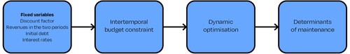
The starting point is the local government’s budget constraints in a two-period setting. (1) $b_1=\left(1+r_0\right)b_0+c_1+m-y_1$(1) (2) $b_2=\left(1+r_1\right)b_1+c_2-y_2=0$(2) $b_t$ is debt at the end of period t. The municipality can borrow in the first period, but the debt must be covered in the second period, hence $b_2=0$. $r_t$ is the interest rate on debt carried over from t to $t+1$, $c_t$ is spending (other than maintenance) in period t, m is maintenance spending in period 1, and $y_t$ is revenues in period t. Consistent with the limited tax discretion in the Norwegian institutional context, we treat local government revenues as exogenous.³ We obtain a consolidated budget constraint by inserting (1) into (2). (3) $c_1+m+{\displaystyle \frac{c_2}{1+r_1}=y_1+{\displaystyle \frac{y_2}{1+r_1}-\left(1+r_0\right)b_0}}$(3)

The consolidated budget constraint states that the present value of spending equals the present value of revenue minus the initial debt. The model focuses on maintenance and disregards investment costs. This implies that we assume that the local government has a fixed building mass (or real capital stock); that is, we consider a situation with a stable population where the need for public buildings does not change over time.

Service provision in period 1 $\left(g_1\right)$ equals current spending, while service provision in period 2 $\left(g_2\right)$ depends on current spending as well as maintenance spending undertaken in period 1. (4) $g_1=c_1$(4) (5) $g_2=f\left(c_2,m\right)$(5) f is a standard production function with constant returns to scale for both inputs. The idea is that, if maintenance is deferred in period 1, it will be necessary to increase current spending in period 2 to maintain service provision in period 2. Several mechanisms might be involved in this process. First, deferred maintenance may increase the level of current spending necessary for proper working of the building mass. Second, deferred maintenance and poor building conditions may lead to health issues, turnover, and sick leave (Buckley et al., 2005) thus increasing labour costs.

The local decision-making is guided by the inter-temporal utility function: (6) $U=u\left(g_1\right)+\delta u\left(g_2\right)$(6) The instantaneous utility function u is strictly concave and δ<1 is a discount factor that captures myopic behaviour. A lower discount factor means that behaviour is more myopic. By maximizing the utility function subject to the budget constraints, we arrive at the following first-order conditions: (7) $u^{\mathrm{\prime }}\left(g_1\right)=\left(1+r_1\right)\delta u^{\mathrm{\prime }}\left(g_2\right)f_c$(7) (8) $f_m=\left(1+r_1\right)f_c$(8) (8) is a condition for cost-efficient production in period 2 (optimal mix of m and $c_2$), whereas (7) is a condition for the optimal allocation of resources across the two periods. The budget constraint (3) and first-order conditions (7) and (8) determine the maintenance and provision of public services in the two periods. We are primarily interested in the solution for maintenance spending which can be summarized as (fully derived in Appendix A): (9) $m=m\left(\begin{array}{c}\delta \\ +\end{array},\begin{array}{c}{y}_1\\ +\end{array},\begin{array}{c}{y}_2\\ +\end{array},\begin{array}{c}{b}_0\\ -\end{array}\right)$(9)

Less myopic behaviour (an increase in the discount factor δ) leads to increased service provision in period 2 at the expense of period 1. Consequently, maintenance spending must be increased in period 1 to achieve cost-efficient production in period 2. In other words, maintenance spending increases and building conditions improve when decision makers become less short-sighted.

The intuition behind the predicted effects of revenue and initial debt is straightforward. Less initial debt and higher revenue (in any of the two periods) have a positive income effect that contributes to increased service provision in both periods, thereby increasing maintenance spending and improving building conditions.

In Appendix A, we derive comparative statistics for the budget deficit. It is an interesting observation that maintenance and deficit move in opposite directions in response to current shocks, that is, when the degree of myopia, period 1 revenues, or initial debt changes. This confirms the similarity between insufficient maintenance and budget deficits; that is, both imply that problems are shuffled ahead.

Institutional background

As in other Scandinavian countries, Norwegian local governments are important providers of welfare services, such as childcare, primary and lower secondary education, primary health care, and care for the elderly. Other important tasks include the culture and infrastructure. The local public sector accounts for around 50% of government consumption, and their revenues make up 18% of GDP. After labour, buildings are probably the most important input in the production of local public services. Local government buildings amount to 50 square meters (m²) per employee and make up as much as a quarter of all non-residential buildings in Norway. Schools make up nearly half of the total building mass and constitute the most important building type, followed by nursing homes (22%), office buildings (11%), and childcare centres (7%).⁴ The main revenue sources for local governments are taxes, central government grants, and user charges. Norwegian local governments have substantial discretion on the expenditure side of their budgets, but their revenues are more regulated. Most taxes are revenue-sharing, and the opportunity to influence current revenues is in practice limited to user charges and property taxes. Property taxes are of little importance, and user charges are either regulated or limited to cover costs.

The political system at the local government level is a representative democracy, in which members of the local council are elected every fourth year. The elections are held on the same day for all the local governments in September. National parties are important players, and the national struggle between socialist and non-socialist camps is mirrored at the local level. Compared with national politics, the main difference is that the majority coalition does not form a cabinet. A typical organization is an alderman model with an executive board and proportional representation from all major parties. The executive board is led by the mayor, and the members of the executive board, including the mayor and deputy mayor, are elected among the members of the local council.

Prior to each fiscal year, the local council made decisions regarding current spending, revenue, investment activity, and borrowing. The executive board and the chief administrative officer (kommunedirektøren) are important players in the early stages of the budgetary process, and the executive board presents a budget proposal to the local council. The parties in the local council are free to put forward their own suggestions, either small or large changes to the proposal from the executive board or totally different budget proposals. Finally, the local council determines the budget either by voting on alternative budget proposals or by issue-by-issue. The final vote takes place shortly before the new year.

Data and empirical specification

Maintenance data

In the empirical analysis, we take advantage of maintenance data from local government accounts in the period 2008–2017. Prior to 2008, local government accounts did not provide an accurate measure of maintenance spending. The problem was that maintenance spending only included materials and labour purchased from external firms and not the maintenance work conducted by local government employees. Since maintenance spending only was captured to the extent that it was outsourced, maintenance was underestimated. Moreover, since local governments outsourced maintenance to different degrees, the data were not comparable across local governments. Since 2008, maintenance work conducted by the local government has been included in maintenance spending and thus captures the actual maintenance activities for all buildings owned by local governments. In this study, we take advantage of this new and improved spending measure.

Evidence of insufficient maintenance in Norway

For the purpose of motivation, we start by presenting maintenance per m² for local public-purpose buildings in Norway. Maintenance spending per m² is the best indicator for evaluating whether maintenance is sufficient. However, it is difficult to develop guidelines for proper maintenance. The traditional engineering approach is to calculate the level of maintenance that is necessary in order to maintain buildings in their original technical condition. The norms for proper maintenance vary according to the type of building and utilization. Available Norwegian guidelines (FOBE, 2006) for local government building mass indicate that maintenance per m² should be Norwegian kroner (NOK) 110–145.⁵ In Panel A of Table 1, we compare the average maintenance spending of local governments with the norm numbers.

Table 1. Comparison of maintenance spending with norm numbers 2008–2017.

Year	NOK pr m2	% of the lower bound of the norm (110 NOK)	% of the upper bound of the norm (145 NOK)
Panel A: Mean maintenance spending compared to norm
2008 (N = 364)	75	68%	52%
2009 (N = 391)	105	95%	72%
2010 (N = 395)	81	74%	56%
2011 (N = 394)	61	55%	42%
2012 (N = 405)	60	55%	41%
2013 (N = 391)	66	60%	46%
2014 (N = 402)	64	58%	44%
2015 (N = 391)	67	61%	46%
2016 (N = 412)	76	69%	52%
2017 (N = 410)	79	72%	54%
Overall (N = 3,955)	73	66%	50%
Panel B: % of observations
	At least at 50% of lower bound	At least at lower bound	At least at upper bound
2008 (N = 364)	43%	13%	8%
2009 (N = 391)	65%	34%	16%
2010 (N = 395)	48%	16%	9%
2011 (N = 394)	38%	8%	4%
2012 (N = 405)	35%	10%	5%
2013 (N = 391)	44%	18%	12%
2014 (N = 402)	41%	16%	11%
2015 (N = 391)	42%	15%	10%
2016 (N = 412)	46%	15%	9%
2017 (N = 410)	48%	16%	8%
Overall (N = 3,955)	45%	16%	9%
Panel C: Maintenance as % of total expenditures
	Mean	Standard deviation
	0.59%	0.35%

Panel A of Table 1 presents the average maintenance spending in local governments in NOK and relative to the norm. In 2008, the local governments spent an average of NOK 75 per m², which amounted to 68% of the lower level of the norm and roughly half of the upper level. In January 2009, a maintenance grant to local governments was implemented as part of a fiscal stimulus package to counteract the impact of the global financial crisis. The grant was earmarked for new maintenance projects that were not included in the budget adopted for 2009. The grant was paid as a flat amount per capita.⁶ The grant contributed to an increase in maintenance spending of NOK 105 per m², that is, 95% to the lower boundary of the norm. After the grant was abolished in 2010, maintenance per m² dropped back to NOK 81 in 2010 and then stabilized in the 60s until increasing to 76 in 2016 and 79 in 2017. Hence, the norm for maintenance spending was, on average, not satisfied in any year in the sample.

Although the averages are well below the norm numbers, a sizable minority of local governments have substantially higher maintenance spending. Panel B lists the share of local governments, at least within the norm numbers. On average, 16% of local governments satisfy the lower bound, while 9% are at least at the upper bound. It is of great interest to investigate the differences between local governments with high and low maintenance levels. In the regression analysis, the main emphasis is on maintenance as a percentage of total expenditures, since these are the variables that most clearly show how much priority local politicians give to maintenance relative to other expenditures. Panel C of Table 1 reports summary statistics for this variable.

Our observation that maintenance in Norwegian local governments is insufficient is consistent with Borge and Hopland (2017). Using survey data on building conditions from 2004, they found that a large proportion of local governments have buildings that are not in satisfying condition. However, the building condition data used in those studies revealed that a sizable minority of local governments have well-maintained buildings.

Econometric specification and hypotheses

In the empirical analysis, we estimate various versions of the regression equation (10) $m_{ijt}={\text{β}}_F\mathit{F}isca{\mathit{l}}_{ijt}+{\text{β}}_P\mathit{P}olitica{\mathit{l}}_{ijt}+{\text{β}}_C\mathit{C}ontrol{\mathit{s}}_{ijt}+{\alpha }_j+{\delta }_t+u_{ijt}$(10) $m_{ijt}$ denotes for the most part maintenance expenditures relative to total expenditures in local government i, in county j, in year t, although we also use maintenance per m² as dependent variable in one of the specifications. $\mathit{F}isca{\mathit{l}}_{ijt}$ is a vector containing indicators of fiscal capacity and stress, $\mathit{P}olitica{\mathit{l}}_{ijt}$ a vector of political variables, and $\mathit{C}ontrol{\mathit{s}}_{ijt}$ a vector of control variables. We control for fixed effects on the regional level (captured by ${\alpha }_j$), by including county dummies in all regressions.⁷ We also include year dummies, capturing the time-fixed effects ${\delta }_t$ in all regressions. $u_{ijt}$ is an error term.

The fiscal variables capture the level of revenue and fiscal distress. From the theoretical model, we derived that local governments with a strong fiscal condition will spend more on maintenance. In addition, we hypothesize that maintenance is more sensitive to fiscal variables than other expenditures are, due to myopic policy. Consequently, we expect a positive coefficient for revenues; that is, maintenance increases (decreases) relatively more than other expenditures when local government revenue increases (decreases). Likewise, we expect negative coefficients for indicators of fiscal distress, and positive coefficients for indicators that are inversely related to fiscal distress.

The main fiscal variable is local government revenue. Because the grant system compensates for unfavourable cost conditions to some extent, nominal per capita revenues may be a poor indicator of ‘real’ revenues (or the service standard that the revenues can generate). This point is illustrated using an example. Consider a small and sparsely populated local government that cannot exploit economies of scale. It will tend to have high nominal revenues per capita because unfavourable cost conditions are compensated through the grant system, but not necessarily high real revenues. As in other recent Norwegian studies (e.g. Borge & Hopland, 2017), we take advantage of an indicator of real per capita revenue published annually by the Ministry of Local Government. The indicator is calculated by ‘deflating’ tax revenues and general-purpose grants using an index of spending needs from the spending needs equalization system. The index for spending needs captures unfavourable cost conditions related to population size, settlement pattern, age composition of the population, and social factors. The indicator of real revenue is an index where the weighted average for all local governments is set to 100 each year. Since most taxes are revenue-sharing and general-purpose grants are distributed by objective criteria, the revenue measure can be considered exogenous (not affected by local government spending priorities) and can be interpreted as an indicator of fiscal capacity. There is substantial variation in fiscal capacity across local governments, reflecting the differences in tax bases and the design of the grant system.

In addition to per capita revenue as an indicator of fiscal capacity, we include indicators of fiscal distress. Fiscal distress is broadly defined as actual fiscal performance in relation to the balanced-budget-rule (BBR). The main requirement of the Norwegian BBR is operational budget balance. In the budget (or ex ante), current revenues must be sufficient to cover current expenditures (wages and materials) and debt servicing costs (net interest payments and instalments on debt). Actual deficits can be carried over, but they must be covered within two years.⁸

The previous year’s net operating surplus⁹ is the first indicator of fiscal distress. Local governments with low or negative net operating surpluses may need to tighten their budgetary policies. However, since the budget can be balanced by the use of rainy-day funds, the need to tighten the budgetary policy will be less for local governments with large funds. The available rainy-day funds by the end of the previous year constitute our second indicator. Both the net operating surplus and rainy-day funds are inversely related to fiscal distress. Moreover, they are measured as % of current revenues.

The final indicator of fiscal distress is a dummy variable that captures whether the local government is included in the Register for State Review and Approval of Financial Obligations (Robek). The register lists local governments that have violated the BBR by passing a budget with a net operating deficit or that have been unable to cover an actual deficit within two years. The most common reason for being registered is that a deficit is not covered on time. The consequence of being registered is that the budget and resolutions to raise new loans must be approved by the county governor, the central government’s representative in the county. Local governments in the register are subject to stronger central government control and must tighten their budgetary policies to be removed from the register.

The fact that politicians face upcoming elections may be a source of myopic policymaking, and the degree of myopic behaviour is likely to increase with electoral uncertainty. Recent papers (Bohn, 2007; Darby et al., 2004; Natvik, 2013) develop models that predict underinvestment in public capital increases when the probability of defeat increases. Because of the similarities between investment and maintenance, we also expect that myopic policymaking will lead to lower maintenance spending.

Borge and Tovmo (2009) analyzed the inter-temporal spending behaviour of Norwegian local governments. They found that political fragmentation is associated with myopic spending behaviour. We use the effective number of parties (ENOP) as an indicator of political fragmentation and myopic behaviour, which is the inverse of the traditional Herfindahl-Hirschman index (11) $ENOP={\left(\sum _{p=1}^{P}S{H}_p^2\right)}^{-1}$(11) where $S{H}_p$ is the share of representatives from party p. The effective number of parties varies from close to 1.1 to nearly 7.4, with an average of 4 (both across local governments and over time). From the theoretical model, we expect a negative coefficient for the effective number of parties, i.e. an increase in political fragmentation leads to a reduction in maintenance relative to other expenditures.

In Norway, the socialist camp is dominated by the Labour Party, whereas the non-socialist camp is more fragmented. Consequently, there is a negative correlation between party fragmentation and the share of socialists on the local council.¹⁰ Hence, we also control for the share of socialists to avoid the coefficient of political fragmentation capturing ideological preferences. Socialist parties are defined as social democrats (The Labour Party) and parties to its left.

The vector of control variables contains the population size and variables that capture the age composition. We include the share of the population below school age (0–5 years), the share of the population in primary and lower secondary schools (6–15 years), and the share of elderly citizens (80 years and above). Since these socioeconomic variables are also included in the spending needs index used to ‘deflate’ local government revenues, they may be less important in our case. We also control for the share of rented building mass because maintenance of rented buildings is not included in the measure of maintenance spending. As climatic conditions can affect the need for maintenance and building conditions, we also included the normal winter temperature in the local governments.

Finally, we include two variables from the survey data in some of the regressions. First, we used self-collected survey data on local government organizations of facility management conducted in 2010 to classify whether the local government uses a centralized or decentralized model for its facilities management. We received responses from 376 local governments (about 88%). Even though the survey was from a particular year, changes in this structure are so rare that the organizational model was most likely the same for almost all local governments throughout the period. The second survey data source was a government commission (NOU, 2004), which was appointed to evaluate facility management in the local public sector. The survey was mailed to all local governments, and 239 (out of 435 at the time of the survey) responded. As part of the survey, respondents were asked to state the extent to which the building mass in general was well maintained. The answer was imposed to be on a 1–6 scale, where 1 is ‘to very little extent’ and 6 ‘to very large extent’. Since the survey was dated several years prior to the start of our sample, we should not face problems with reverse causality, even though maintenance expenditures obviously affect current and future building conditions. Since the number of observations is limited in the two surveys, we exclude these variables from most regressions.

Main results

Table 2 presents the main results. In column (A), we include local government revenue and the effective number of parties, and only control for political ideology, the share of rented buildings, population size, and county fixed effects. Local government revenue is strongly significant with the expected positive sign; that is, maintenance expenditures are more sensitive to revenue changes than other expenditures. The coefficient indicates that local governments that increase their revenues by the sample standard deviation will increase maintenance expenditures as a share of total expenditures by approximately 30% of the standard deviation for the dependent variable. Hence, the effect is not only statistically significant but also economically significant.

Table 2. Main results.

Maintenance measured	(A)	(B)	(C)	(D)	(E)	(F)	(G)	(H)
	As % of total expenditures	Per m^2 (in 1,000 NOK)	As % of total expenditures	As % of total expenditures	As % of total expenditures	As % of total expenditures	As % of total expenditures	As % of total expenditures
Local government	0.00507***	0.474***	0.00506***	0.00506***	0.00408***	0.00417***	0.00386**	0.00320*
revenue	(0.00134)	(0.127)	(0.00160)	(0.00134)	(0.00147)	(0.00152)	(0.00153)	(0.00164)
Surplus in year t-1			0.00557
(% of revenues)			(0.00372)
Robek				−0.0155
				(0.0338)
Rainy-day funds					0.00691**	0.00654**	0.00713**	0.00477
(% of revenues)					(0.00320)	(0.00317)	(0.00333)	(0.00350)
Effective number	−0.0346*	−1.117	−0.0344*	−0.0341*	−0.0325*	−0.0288	−0.0274	−0.0244
of parties	(0.0183)	(1.921)	(0.0188)	(0.0182)	(0.0182)	(0.0189)	(0.0192)	(0.0276)
Share of socialists	0.000260	0.0351	0.000377	0.000244	0.000437	0.000665	0.000378	0.00125
in the local council	(0.00133)	(0.150)	(0.00142)	(0.00133)	(0.00132)	(0.00136)	(0.00132)	(0.00184)
Population size	0.00701*	2.721***	0.00529	0.00694*	0.00714*	0.00861**	0.00938**	0.00813*
(in 10,000)	(0.00411)	(0.706)	(0.00384)	(0.00412)	(0.00392)	(0.00426)	(0.00447)	(0.00462)
Rented buildings (%)	−0.00442***	0.442	−0.00447***	−0.00439***	−0.00413***	−0.00393***	−0.00332**	−0.00350***
	(0.00101)	(0.420)	(0.00114)	(0.00101)	(0.00103)	(0.00106)	(0.00139)	(0.00112)
Share of population						0.0136	0.0318	−0.00714
0–5 years (%)						(0.0194)	(0.0215)	(0.0282)
Share of population						0.00477	0.000977	−0.0143
6–15 years (%)						(0.0176)	(0.0167)	(0.0255)
Share of population						0.0268	0.0312	0.0137
80 years and above (%)						(0.0187)	(0.0199)	(0.0245)
Normal winter						0.00629	0.000492	0.00458
temperature						(0.00778)	(0.00696)	(0.0110)
Centralized facility							−0.0393	−0.0963
management							(0.0694)	(0.0975)
Building conditions								0.0582*
in 2004								(0.0300)
Observations	3948	3927	3584	3947	3946	3918	3456	1951
R-squared	0.098	0.077	0.105	0.099	0.106	0.109	0.117	0.165

Constant terms, county dummies, and year dummies (not reported) were included. Robust standard errors (clustered at the local government level) are in parentheses. ***p < 0.01, **p < 0.05, *p < 0.1.

The effective number of parties is also statistically significant. This negative sign is consistent with the hypothesis that myopic politicians tend to reduce maintenance relative to other expenditures. The coefficient indicates that a reduction in political fragmentation by one standard deviation is associated with an increase in maintenance expenditures as a share of the total expenditure of about 10% of a standard deviation.

The share of rented buildings comes out as highly significant and with the expected negative sign. We also observe that more populous local governments seem to give maintenance a higher priority than smaller local governments. The share of socialists in the local council is statistically insignificant.

In Column (B), we estimate the same specification but use maintenance per m² as the dependent variable. Again, the coefficient for local government revenue comes out as significantly positive. The coefficient for party fragmentation is still negative but is far from significant at any conventional level. This indicates that, while maintenance is more sensitive to political fragmentation than other expenditures, political fragmentation does not affect the amount of maintenance spent per unit of building mass. Further, we observe that populous local governments tend to spend more on maintenance per m² than less populated ones. We also note that the share of rented buildings is insignificant in this regression, which is unsurprising because the dependent variable in this specification only considers the building mass owned by the local government.

In columns (C)–(E), we include the three indicators of fiscal distress individually. The coefficients for the lagged surplus [Column (C)] and Robek [Column (D)] come out with the expected sign but are not significant at conventional levels. Rainy-day funds come out as significant and with the expected positive sign; that is, local governments with small funds cut down on maintenance relative to other expenditures. The effects of local government revenue and the effective number of parties are largely unaffected by the inclusion of fiscal distress indicators.

Column (F) shows the set of demographic and climatic controls. These mostly come out as insignificant and, more importantly, do not affect the coefficients for local government revenue, and political fragmentation is not much affected. However, a slight decrease in the coefficient combined with a small increase in the estimated standard error is sufficient to make the effective number of parties fall short of statistical significance.

In Column (G), we extend the regression with a dummy for centralized facilities management. This also comes out as insignificant and has no effect on the coefficients for revenue and political strength. In the final extension in Column (H), we added the building conditions in 2004. This comes out as significantly positive, indicating that the local governments that prioritize maintenance in the sample period were probably the same as those prior to the 2004 survey. The coefficients for local government revenue and political fragmentation remain quite stable, but the standard errors for political fragmentation increase a bit so that it just falls short of significance. This may reflect that building conditions pick up the effect of political fragmentation.

In Table 3, we study heterogeneity in the results across local governments with different real revenue levels and trends. We expect that local governments with low or declining revenues will find it even more challenging to prioritize maintenance than other local governments. In Columns (A) and (B), we split the sample according to local government revenue. We observe that the effect from revenues is substantially stronger in local governments with low revenues. Further, political fragmentation affects maintenance expenditures only in low-income local governments. Hence, it seems that it becomes increasingly difficult to prioritize maintenance as the local government’s economy deteriorates. In Columns (C) and (D), we split observations by whether local governments experienced a reduction in real revenue from one year to the next. We observe that the revenue effect is actually stronger in local governments that do not experience a decline in revenues. We also see that political fragmentation is significant only for local governments, with a reduction in revenue.

Table 3. Heterogeneous effects for local governments with different income levels and development.

Maintenance measured	(A)	(B)	(C)	(D)
	As % of total expenditures	As % of total expenditures	As % of total expenditures	As % of total expenditures
Local government	0.00500***	0.00337**	0.00291**	0.00486***
revenue	(0.00189)	(0.00156)	(0.00114)	(0.00170)
Rainy-day funds	0.0103***	0.00455	0.00672*	0.00715**
(% of revenues)	(0.00261)	(0.00469)	(0.00345)	(0.00357)
Effective number	−0.0327	0.0106	−0.0467*	−0.0222
of parties	(0.0203)	(0.0279)	(0.0255)	(0.0170)
Share of socialists	−0.00148	0.00278	0.00108	0.000273
in the local council	(0.00190)	(0.00195)	(0.00178)	(0.00128)
Population size	0.0130***	−0.516*	0.0103	0.00671*
(in 10,000)	(0.00443)	(0.269)	(0.00688)	(0.00392)
Rented buildings (%)	−0.00320***	−0.00310	−0.00451***	−0.00397***
	(0.00107)	(0.00316)	(0.00121)	(0.00127)
Observations	1988	1958	1106	2840
R-squared	0.158	0.104	0.103	0.117
	Below median	Above median	Reduced real income	At least the same real income
	average income	average income	from t-1 to t	in t as in t-1

Constant terms, county dummies, and year dummies (not reported) were included. Robust standard errors (clustered at the local government level) are in parentheses. ***p < 0.01, **p < 0.05, *p < 0.1.

Robustness analysis

The substantial change in the reporting system for maintenance expenditures from 2008 onwards makes us particularly concerned about outliers. In particular, we might see under-reporting of maintenance expenditures in some local governments if they do not fully adapt to the new system from the start. This section aims to study how this may have affected our main results. Populous and urban local governments have larger administrations than smaller ones and are thus likely to be able to implement changes quickly. In Table 4, we omit local governments with fewer than 1500 inhabitants in column (A), less than 7000 in column (B), and less than 13,000 in column (C). This amounts to a reduction in the sample by approximately 15%, 65%, and 80%, respectively. The sign and significance of the three variables of main interest–local government revenue, rainy-day-funds, and the effective number of parties–are unaffected by this reduction in the number of observations. However, it is interesting to note that the quantitative effects increase substantially when we restrict the sample to fewer observations.

Table 4. Omitting small local governments

	(A)	(B)	(C)
Maintenance measured	As % of total expenditures	As % of total expenditures	As % of total expenditures
Local government	0.00347**	0.00606**	0.00941*
revenue	(0.00158)	(0.00265)	(0.00558)
Rainy-day funds	0.00519**	0.00564*	0.00529*
(% of revenues)	(0.00253)	(0.00296)	(0.00313)
Effective number	−0.0373**	−0.0632***	−0.0735**
of parties	(0.0175)	(0.0241)	(0.0289)
Share of socialists	−0.00180	−0.000199	0.00208
in the local council	(0.00131)	(0.00216)	(0.00264)
Population size	0.00861**	0.0132***	0.00636*
(in 10,000)	(0.00400)	(0.00411)	(0.00356)
Rented buildings (%)	−0.00394***	−0.00419***	−0.00371***
	(0.00103)	(0.000700)	(0.000885)
Observations	3323	1341	793
R-squared	0.094	0.199	0.279
Omitted observations	Population < 1500	Population < 7000	Population < 13,000

Constant terms, county dummies, and year dummies (not reported) were included. Robust standard errors (clustered at the local government level) are in parentheses. ***p < 0.01, **p < 0.05, *p < 0.1.

As a second robustness test, in Table 5, we omit outliers in reported maintenance expenditures since these might be due to misreporting or special circumstances. In Column (A), we exclude all observations with maintenance expenditures below 20 NOK per m², i.e. about 10% of the total observations. Column (B) excludes all observations with maintenance expenditures above NOK 140 per m², again about 10% of the total observations. In Column (C), we exclude those with high and low maintenance expenditures. In these cases, the quantitative effects are reduced but the precision of the estimates increases.

Table 5. Omitting maintenance expenditure outliers

Maintenance measured	(A)	(B)	(C)
	As % of total expenditures	As % of total expenditures	As % of total expenditures
Local government	0.00406***	0.00109**	0.00107**
revenue	(0.00148)	(0.000469)	(0.000448)
Rainy-day funds	0.00574*	0.00656***	0.00566***
(% of revenues)	(0.00323)	(0.00188)	(0.00184)
Effective number	−0.0336*	−0.0195*	−0.0195*
of parties	(0.0190)	(0.0101)	(0.00993)
Share of socialists	0.000346	−8.65e−05	−0.000133
in the local council	(0.00135)	(0.000755)	(0.000724)
Population size	0.00460	0.00985***	0.00784***
(in 10,000)	(0.00356)	(0.00348)	(0.00291)
Rented buildings (%)	−0.00479***	−0.00469***	−0.00543***
	(0.00104)	(0.00137)	(0.00128)
Observations	3588	3540	3182
R-squared	0.108	0.114	0.117
Omitted observations	<NOK 20 per m^2	>NOK 140 per m^2	<NOK 20 per m^2 & >NOK 140 per m^2

Constant terms, county dummies, and year dummies (not reported) were included. Robust standard errors (clustered at the local government level) are in parentheses. ***p < 0.01, **p < 0.05, *p < 0.1.

Concluding remarks

In this paper, we have shown that maintenance expenditures are below norms for good maintenance and depend on fiscal and political characteristics of Norwegian local governments. An interesting analogue is drawn to budget deficits, and we show that theoretically, these policy problems are very similar. This is also supported by our empirical results, which find very similar determinants for poor maintenance as earlier studies have found for budget deficits. Hence, we conclude that the ability to prioritize maintenance is determined by many of the same local government characteristics that are known to affect deficits.

Maintenance is important both for preserving the value of the building stock and ensuring that the buildings are in sufficient condition to serve their purpose in service production. Hence, one should think of ways to put a wedge between economic and political factors and maintenance. A method that has gained popularity in Norwegian local governments in recent years is to establish units that are responsible for maintenance. Such units can be organized in different ways. One alternative is to have separate organizations for service provision (school, childcare centres, nursing homes, etc.) and a maintenance unit and with separate budgets and no transactions between them. Another alternative is to establish models where the service providers pay rent to the unit responsible for maintenance. The rent, which is supposed to cover maintenance, is based on a contract between the maintenance unit and the local government. The establishment of units that are responsible for maintenance makes it more difficult for local politicians to make short-sighted cuts in maintenance expenditures. Moreover, with a unit that is responsible for maintenance local politicians face a professional real estate manager who might be better able to present the needs and challenges in managing the public buildings than the leaders for service provision. Whether units responsible for maintenance are better able to maintain public buildings is ultimately an empirical question, and it is a clear limitation for our study that we are unable to evaluate this question with the data we have. We encourage further empirical research into this question.

On the theory side, this paper has made significant contributions by providing a formal mathematical model with the purpose of guiding the empirical analyses. The model emphasizes the role of maintenance as an input in the production of public services. A potential weakness of the theoretical approach is that there is only a single actor, the local government, that makes decisions. It will be interesting to extend the theoretical model to also include several actors like local politicians, local administrators, service providers, and ultimately the citizens who benefit from well-maintained buildings. A fruitful direction to consider is to use game theory to analyze possible conflicts of interest and how these conflicts can be mitigated through organizational design. Relevant literature includes Chan and Mestelman (1988), Dixit (2002), and Cohen et al. (2021).

Acknowledgements

Earlier versions of this paper have been presented at seminars at the Norwegian University of Science and Technology, University of Maryland College Park, and Oslo Metropolitan University. We are grateful for the comments from the participants.

Disclosure statement

No potential conflict of interest was reported by the authors.

Data availability statement

The data that support the findings of this study are available from the corresponding author upon reasonable request.

Additional information

Funding

Borge is grateful for funding from the Norwegian Research Council through the project Water, Sewage, and Health (WaSH), project number 326301.

Notes

1 A similar examination is carried out by Rattsø (1999) on Norwegian data. As Holtz-Eakin and Rosen (1989, 1993) he cannot reject that local public investments are determined by rational forward-looking behaviour.

2 See McGrattan and Schmitz (1999) for a discussion of the difficulties of constructing measures of maintenance.

3 The predictions for maintenance would be the same if the model was extended to allow for local tax discretion.

4 Around half of all childcare centres are privately owned and are not included in the figures.

5 The original numbers from 2004 are adjusted for inflation and are in fixed 2008 prices, as are all other numbers in the paper. It is worth noting that it is not clear-cut how such norm numbers are best defined. In 2017, the last year of our study, one EURO was on average worth NOK 9.33.

6 The scope of the maintenance grant was broader than the spending concept used in this study. The grant could be used for local government infrastructure (not only buildings), for private organizations receiving financial support from the local government, and for renovation and upgrading.

7 There were 19 counties in Norway during the period of study. Each county has an average of around 23 local governments.

8 An actual deficit is covered when future surpluses are at least as large as the deficit.

9 The net operating surplus is current revenue less current expenditures and debt servicing costs.

10 The correlation between the effective number of parties and the share of socialists is −0.33.

Appendices

Appendix A: Comparative statics

This appendix presents the comparative static results presented in Section 2. The points of departure are the first-order conditions (7)–(8) and the consolidated budget constraint (3). The comparative statics for maintenance are given by: (A1) ${\displaystyle \frac{\mathrm{\partial }m}{\mathrm{\partial }\delta }={\displaystyle \frac{u^{\mathrm{\prime }}\left(g_2\right)f_m}{D{f}_c}(f_{cc}{f}_m-f_{cm}{f}_c)>0}}$(A1) (A2) ${\displaystyle \frac{\mathrm{\partial }m}{\mathrm{\partial }{y}_1}=-{\displaystyle \frac{u^{\mathrm{\prime }}\mathrm{\prime }\left(g_1\right)}{D{f}_c}(f_{cc}{f}_m-f_{cm}{f}_c)>0}}$(A2) where $D=-\left[\frac{u^{\mathrm{\prime }}\mathrm{\prime }\left(g_1\right)}{f_c{f}_m}+{\displaystyle \frac{f_m}{f_c}\delta u^{\mathrm{\prime }}\mathrm{\prime }\left(g_2\right)}\right](f_{cc}{f}_m^2-2f_{cm}{f}_c{f}_m+f_{mm}{f}_c^2)$ is negative from the second-order condition. The terms within the parentheses on the right-hand sides of (A1) and (A2) are negative, given that maintenance is a normal factor of production. It is evident from equation (3) in the main text that increased revenues in period 2 have the same qualitative effect on maintenance as increased revenues in period 1 $\left(\frac{\mathrm{\partial }m}{\mathrm{\partial }{y}_2}>0\right)$, whereas higher initial debt has the opposite effect, $\left(\frac{\mathrm{\partial }m}{\mathrm{\partial }{b}_0}<0\right)$.

The comparative statics for the budget deficit, $d=c_1+m-y_1$, is given by (A3) ${\displaystyle \frac{\mathrm{\partial }d}{\mathrm{\partial }\delta }=-{\displaystyle \frac{u^{\mathrm{\prime }}\left(g_2\right)}{D}(f_{mm}{f}_c-f_{cm}{f}_m)<0}}$(A3) (A4) ${\displaystyle \frac{\mathrm{\partial }d}{\mathrm{\partial }{y}_1}={\displaystyle \frac{u^{\mathrm{\prime }}\mathrm{\prime }\left(g_1\right)}{D{f}_m}(f_{mm}{f}_c-f_{cm}{f}_m)<0}}$(A4) The effects of revenues in period 2 and the initial debt are straightforward. Increased revenues in period 2 have a positive income effect, which increases both $c_1$ and m, and then it follows that $\frac{\mathrm{\partial }d}{\mathrm{\partial }{y}_2}>0$. A higher initial debt has a negative income effect that reduces both $c_1$ and m, and then it follows that $\frac{\mathrm{\partial }d}{\mathrm{\partial }{b}_0}>0$.

Appendix B: Descriptive statistics for the explanatory variables, maintenance regressions

Table

Variable	Description	Mean (st.dev)
Local government revenue	The sum of local taxes and lump-sum grants from the central government. Measured per capita and adjusted for spending needs. Normalized such that the weighted average (for all local governments) equals 100 each year.	107.71 (20.84)
Effective number of parties	An indicator of party fragmentation in the local council.	3.99 (1.05)
Share of socialists in the local council	The share (%) of socialists in the local council.	35.34 (14.13)
Previous surplus	The net operating surplus the previous year. Measured in % of current revenues.	2.47 (3.92)
Rainy-day-funds	Available funds by the end of the previous fiscal year. Measured in % of current revenues.	6.95 (7.43)
Central government control (Robek)	A dummy variable set equal to one if the local government is listed in the Register of State Review and Approval of Financial Obligations.	0.11 (0.31)
Rented buildings	The share (%) of the building mass that is rented.	3.08 (8.28)
Population size	The number of inhabitants January 1, in ten thousands.	1.04 (2.12)
Share of population 0–5 years	The share (%) of the population 0–5 years January 1.	6.57 (1.24)
Share of population 6–15 years	The share (%) of the population 6–15 years January 1.	12.50 (1.46)
Share of population 80 years and above	The share (%) of the population 80 years and above January 1.	5.38 (1.47)
Normal winter temperature	Average winter temperature 1998–2003.	−3.01 (4.05)
Centralized facility management	Dummy equal to one if the local government has a centralized facility management unit in 2010.	0.87 (0.34)
Initial building condition	The local governments building condition in 2004. Reported on a 1–6 scale where 1 indicates very poor conditions and 6 very good conditions.	3.11 (1.09)

References

- Bohn, F. (2007). Polarisation, uncertainty and public investment failure. European Journal of Political Economy, 23(4), 1077–1087. https://doi.org/10.1016/j.ejpoleco.2006.11.004
- Borge, L.-E., & Hopland, A. O. (2017). Schools and public buildings in decay: The role of political fragmentation. Economics of Governance, 18(1), 85–105. https://doi.org/10.1007/s10101-016-0187-z
- Borge, L.-E., & Tovmo, P. (2009). Myopic or constrained by balanced-budget rules? The intertemporal spending behavior of Norwegian local governments. Finanz-Archiv, 65(2), 200–219. https://doi.org/10.1628/001522109X466518
- Buckley, J., Schneider, M., & Shang, Y. (2005). Fix it and they might stay: School facility quality and teacher retention in Washington D.C. (Vol. 107, pp. 1107–1123). The Teachers College Record.
- Chan, K. S., & Mestelman, S. (1988). Institutions, efficiency and the strategic behavior of sponsors and bureaus. Journal of Public Economics, 37(1), 91–102. doi:https://doi.org/10.1016/0047-2727(88)90006-0
- Cohen, C., Halfon, E., & Schwartz, M. (2021). Trust between municipality and residents: A game-theory model for municipal solid-waste recycling efficiency. Waste Management, 127, 30–36. https://doi.org/10.1016/j.wasman.2021.04.018
- Darby, J., Li, C.-W., & Muscatelli, V. A. (2004). Political uncertainty, public expenditure and growth. European Journal of Political Economy, 20(1), 153–179. https://doi.org/10.1016/j.ejpoleco.2003.01.001
- De Haan, J., Sturm, J. E., & Sikken, B. J. (1996). Government capital formation: Explaining the decline. Weltwirtschaftliches Archiv, 132(1), 55–74. https://doi.org/10.1007/BF02707902
- Dixit, A. (2002). Incentives and organizations in the public sector: An interpretative review. The Journal of Human Resources, 37(4), 696–727. https://doi.org/10.2307/3069614
- FOBE. (2006). Kartlegging av kommunenes utgifter til vedlikehold av sine bygninger [A survey of local government maintenance spending]. Norwegian Association of Municipal Engineers.
- Holtz-Eakin, D., & Rosen, H. S. (1989). The “rationality” of municipal capital spending. Regional Science and Urban Economics, 19(3), 517–536. https://doi.org/10.1016/0166-0462(89)90017-3
- Holtz-Eakin, D., & Rosen, H. S. (1993). Municipal construction spending: An empirical examination. Economics and Politics, 5(1), 61–84. https://doi.org/10.1111/j.1468-0343.1993.tb00068.x
- Hulten, C. R., & Peterson, G. E. (1984). The public capital stock: Needs, trends, and performance. American Economic Review (Papers and Proceedings), 74(2), 166–173.
- Inman, R. P. (1983). Anatomy of a fiscal crisis. Business Review (Federal Reserve Bank of Philadelphia), September–October, 15–22.
- McGrattan, E. R., & Schmitz, J. A. (1999). Maintenance and repair: Too big to ignore. Quarterly Review, 23(4), 2–13. https://doi.org/10.21034/qr.2341
- Natvik, G. J. (2013). The political economy of fiscal deficits and government production. European Economic Review, 58(1), 81–94. https://doi.org/10.1016/j.euroecorev.2012.12.001
- NOU (2004). Velholdte bygninger gir mer til alle (Well maintained buildings is better for all) (Report). Government Administration Services, Oslo.
- Oxley, H., & Martin, J. P. (1991). Controlling government spending and deficit: Trends in the 1980s and prospects for the 1990s. OECD Economic Studies, 17, 145–189.
- Poterba, J. M. (1995). Capital budgets, borrowing rules, and state capital spending. Journal of Public Economics, 56(2), 165–187. https://doi.org/10.1016/0047-2727(94)01431-M
- Rattsø, J. (1999). Aggregate local public sector investment and shocks: Norway 1946–1990. Applied Economics, 31(5), 577–584. https://doi.org/10.1080/000368499324020
- Roubini, N., & Sachs, J. D. (1989). Government spending and budget deficits in the industrial countries. Economic Policy, 4(8), 99–132. https://doi.org/10.2307/1344465
- Sturm, J.-E. (1998). Public capital expenditures in the OECD countries: The causes and impact of the decline in public capital spending. Edward Elgar Publishing.