On the systemic entropy of low-order systems

Abstract

Reliability engineering is a well-defined field and systemic analysis is not new. Typically, the first raw-moment (MTTF) is all that is sought in applications of this method and a rule-of-thumb method achieves this algebraically without the need for calculus by assuming exponential distributions. However, there is no standard labelling or naming of the different block diagrams used, nor is there a standard list of solutions for low-order networks. In this paper different moments are compared, and the vector algebra approach is emphasised. A small amount of fine structure is evident in the moments, but broadly they are found to be equivalent for bulk system analysis. Analogy is made to statistical physics and a set of characteristic values is developed.

Keywords:

• Reliability engineering
• mean time to failure
• entropy
• systemic analysis

1. Summary of reliability engineering theory

It is hypothesised that any system/process can be subdivided into parts connected in a network which can be represented two-dimensionally. The reliability of the entire system is then a combination of the reliability of the parts (Saleh & Marais, 2006). Whilst it is not an essential assumption, it is usual that each sub-system or component has only two states: working or broken; reliable R, or failed F. The probability of each state $P\left(R\right),\mathrm{ }P\left(F\right)$ is abbreviated here as simply $R,$ and $F.$ If a non-critical subsystem fails, but not the entire system; then the chance of total system failure changes. This is not the same thing as a continuous production operation producing a lower quality output. (1) $$R+F=1$$(1)

The simplest network is of a single black-box as shown on Figure 1.

Figure 1. Black-box network.

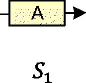
For the example of Figure 1, we might have a system with 90% reliability R = 0.9, and 10% unreliability F = 0.1 using (1). This simple formulation works easily for such a problem as rolling a six-sided die and defining a ‘6’ result as operating and all other results as failures. When describing a more sophisticated system, such as a desktop computer, house, etc. then the reliability relates to an unrepairable failure in the normal operating lifespan. Such thinking leads naturally into discussion of failure rates and average lifespans. These are understood to be moments of some probability distribution as a function of time. There are infinitely many probability distributions, but engineering practice is constrained by two principles in its choice of which to use. Firstly, the engineer is usually conversant with only a handful of the simplest functions such as polynomials and exponentials, for which calculus is easy. Secondly some distributions pertain to a physical cause: The Gaussian bell-curve describes a diffusion process, top-hat for white-noise, binomial relates to permutations and combinations, Poisson for rare events, the Weibull for mechanical fracture and the extreme-order to tail-end phenomenon. However, most applications of reliability engineering use the exponential for the simplicity of single-parameter sampling. (2) $$R=e^{-{\left(t/s\right)}^{\beta }}$$(2)

The Weibull probability distribution (2) is in general a 3-parameter distribution (i.e. replace t by t − τ where τ is the start time), s is the scale factor (for example quantifying time t in hours or years) and β is the shape factor. The exponential distribution is simply (2) in the special case β = 1 applied to the ‘normal working life’ of a system. In that case, λ = 1/s is the failure rate for a mean time to failure. (3) $$R=e^{-\lambda t}$$(3)

On Figure 2 the two-block networks can be seen and the basic ideas of series and parallel (also known as Redundant) operations in a process.

Figure 2. Series (left) and parallel (right) networks.

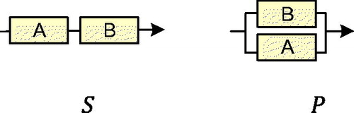
Considering the series system first; the system can only function if both sub-systems A ‘AND’ B are functioning. The word ‘AND’ being mathematically equivalent to multiplication we obtain the system total reliability as a ‘structure function’ of the failure rates of the subnets (4)(4) $$R_T=R_A{R}_B=e^{-{\lambda }_{A}t}{e}^{-{\lambda }_{B}t}=e^{-\left({\lambda }_A+{\lambda }_B\right)t}$$(4) . (4) $$R_T=R_A{R}_B=e^{-{\lambda }_{A}t}{e}^{-{\lambda }_{B}t}=e^{-\left({\lambda }_A+{\lambda }_B\right)t}$$(4)

This leads easily to computing the expected failure time (5)(5) $$\mathit{mttf}=\overline{t}=\underset{-\mathrm{\infty }}{\overset{\mathrm{\infty }}{\int }}tf\mathrm{d}t=\underset{0}{\overset{\mathrm{\infty }}{\int }}{R}_{T}dt=\underset{0}{\overset{\mathrm{\infty }}{\int }}{e}^{-\left({\lambda }_A+{\lambda }_B\right)t}dt=\frac{1}{\left({\lambda }_A+{\lambda }_B\right)}$$(5) from the probability density function $f=dF/dt.$ (5) $$\mathit{mttf}=\overline{t}=\underset{-\mathrm{\infty }}{\overset{\mathrm{\infty }}{\int }}tf\mathrm{d}t=\underset{0}{\overset{\mathrm{\infty }}{\int }}{R}_{T}dt=\underset{0}{\overset{\mathrm{\infty }}{\int }}{e}^{-\left({\lambda }_A+{\lambda }_B\right)t}dt=\frac{1}{\left({\lambda }_A+{\lambda }_B\right)}$$(5)

In this simple case the mean time to failure equates to the sum of the individual failure rates. The same can be said for series with more than two components. For the parallel system on Figure 2 the same procedure can be followed to obtain (6)(6) $$R_T=e^{-{\lambda }_{A}t}+e^{-{\lambda }_{B}t}-e^{-\left({\lambda }_A+{\lambda }_B\right)t}$$(6) (6) $$R_T=e^{-{\lambda }_{A}t}+e^{-{\lambda }_{B}t}-e^{-\left({\lambda }_A+{\lambda }_B\right)t}$$(6) and (7) $$\mathit{mttf}=\frac{1}{{\lambda }_A}+\frac{1}{{\lambda }_B}-\frac{1}{\left({\lambda }_A+{\lambda }_B\right)}$$(7)

Immediately one sees that the mttf can be obtained from the structure function by replacing exponentials by reciprocals and sums. This is similar to the laws of indices and is a good case for engineers to only use the exponential probability distribution.

If one knows the failure rates (also known as hazard rates) for use in Equations (6)(6) $$R_T=e^{-{\lambda }_{A}t}+e^{-{\lambda }_{B}t}-e^{-\left({\lambda }_A+{\lambda }_B\right)t}$$(6) and (7)(7) $$\mathit{mttf}=\frac{1}{{\lambda }_A}+\frac{1}{{\lambda }_B}-\frac{1}{\left({\lambda }_A+{\lambda }_B\right)}$$(7) , then the inverse problem is to select a value of time ‘t’ corresponding to a particular reliability $R_T\in \left\{0.68,0.95,0.997\right\}$ which are of course values ingrained when learning about (totally unconnected) Gaussian-symmetrical problems.

The value of ‘t’ from (6)(6) $$R_T=e^{-{\lambda }_{A}t}+e^{-{\lambda }_{B}t}-e^{-\left({\lambda }_A+{\lambda }_B\right)t}$$(6) is not trivially obtained by algebra. Either it is read from a graph-plot or the one-block estimate (3) is used in the form $t=-ln\left(R\right)/\lambda$ where $\lambda =1/\mathit{mttf}$ is an estimated bulk or characteristic-failure rate and equivalently a characteristic time for failures and repairs (Sifonte & Reyes-Picknell, 2017).

For systemic analysis we treat all the hazard rates as equal ${\lambda }_A={\lambda }_B=\dots =\lambda$ so that Equations (4)–(7) become (8)(8) $$\begin{array}{cc}\mathrm{S}\mathrm{eries}& \mathrm{P}\mathrm{arallel}\\ R=x^2, \mathit{mttf}=\frac{1}{2\lambda }& R=2x-x^2, \mathit{mttf}=\frac{3}{2\lambda } \end{array}$$(8) where $x=e^{-\lambda t}$ for brevity. (8) $$\begin{array}{cc}\mathrm{S}\mathrm{eries}& \mathrm{P}\mathrm{arallel}\\ R=x^2, \mathit{mttf}=\frac{1}{2\lambda }& R=2x-x^2, \mathit{mttf}=\frac{3}{2\lambda } \end{array}$$(8)

2. Names and labels for the different networks

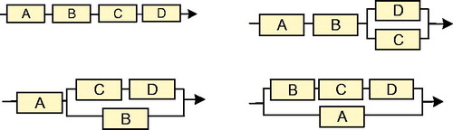
To distinguish the two networks, we do not have particular names and there is no database or standard list of networks, names and their properties. Since Figure 1 shows the one block network, and Figure 2 the two possible two-block networks, shown on Figure 3 are the four possible three block networks. Labelled pictures for n = 1 to 5 are given as Table A1 in the Appendix.

Figure 3. Three block networks with labels.

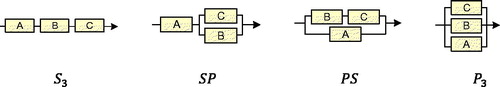
This can be developed from the simplest networks and extended as more complicated examples are worked into a simple list. To that extent, comparing Figures 1 and 2 the reader will imagine a simple chain of n-blocks in a series. Such can be denoted S_n. Similarly, n-blocks in parallel can be denoted P_n. Since the basic building unit of higher order networks is combinations of two or more things, there is no need to use a suffix ‘2’ for two blocks. This is to say that the simple series of 1, 2, 3, etc blocks can be denoted S₁, S, S₃, … S_n. This explains the labelling used on Figures 1, 2 and part of Figure 3. But it is necessary to explain also how SP and PS are chosen on Figure 3.

Every network has a ‘structure function’ which formulaically expresses the combination reliability in terms of the parts. This can be obtained using the ‘top down’ method by iteratively applying three system laws:

1. Continuity $R+F=1$ for any system or subsystem

2. Series rule $R_S=R_1{R}_2$

3. Parallel rule $F_P=F_1{F}_2$

The continuity of probability requires a system to be either failed or reliable. This rule can be easily relaxed, but that is beyond this paper for example to account for ‘spurious’ failures. The series rule is easily understood from Figure 2 considering electric current flowing down a wire with two light bulbs connected in series. For the entire system to be ‘alight’ both bulbs must be functioning. The reliability of the system is equal to the reliability of bulb 1 ‘AND’ bulb 2. The AND operator being equivalent to multiplication. Similarly, for the parallel system of Figure 3 and rule 3, there are no lights (total system failure) only if there is failure of bulb 1 ‘AND’ bulb 2.

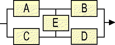
Consider the SP-labelled network of Figure 3, where A, B, and C refer to the components and $R_X$ is the reliability of component ‘X’ (probability it will operate correctly upon demand). (9) $$R_T=R_{\mathit{ABC}}$$(9) ‘total/system reliability equals the reliability due to the components A, B, C, D and E’. A suffix T is used in (9) for the total/system to avoid confusion with a series configuration (S and P suffices used throughout this paper). (10) $$\begin{array}{cc}=R_A{R}_{BC}& \text{rule}\mathrm{ }2\\ =R_A\left(1-F_{BC}\right)& \text{rule}\mathrm{ }1\\ =R_A\left(1-F_B{F}_C\right)& \text{rule}\mathrm{ }3\\ =R_A\left(1-\left(1-R_B\right)\left(1-R_C\right)\right)& \text{rule}\mathrm{ }1\end{array}$$(10)

For a network that is overall a series the sequence of rules is 2–1–3–1– repeatedly, for a parallel network the sequence is 1–3–1–2– (out of phase). This sequence has a mnemonic ‘STOP’ for ‘series-starts-2 but start-1 for parallel’.

As a time dependent function of failure rates $R_x=e^{-{\lambda }_{x}t}$ (11) $$R_T=e^{-{\lambda }_{A}t}\left(1-\left(1-e^{-{\lambda }_{B}t}\right)\left(1-e^{-{\lambda }_{C}t}\right)\right)$$(11) (12) $$R_T=e^{-\left({\lambda }_A+{\lambda }_B\right)t}+e^{-\left({\lambda }_A+{\lambda }_C\right)t}-e^{-\left({\lambda }_A+{\lambda }_B+{\lambda }_C\right)t}$$(12) (13) $$\mathit{mttf}=\frac{1}{{\lambda }_A+{\lambda }_B}+\frac{1}{{\lambda }_A+{\lambda }_C}-\frac{1}{{\lambda }_A+{\lambda }_B+{\lambda }_C}$$(13)

Then the characteristic failure rate is $\lambda =1/\mathit{mttf}$ and $t=-ln\left(R\right)/\lambda .$ For assuring a 95% system reliability $ln\left(0.95\right)\approx 0.051.$ The scheduled time until replacement would be (14) $$t_{\mathit{maintenance}}\approx \frac{\mathit{mttf}}{20}$$(14)

Note that MTTF is used to characterise non-repairable systems/components where the strategy is run-to-failure rather than repair. In ‘shorthand’ form, dropping the suffix notation, Equation (10)(10) $$\begin{array}{cc}=R_A{R}_{BC}& \text{rule}\mathrm{ }2\\ =R_A\left(1-F_{BC}\right)& \text{rule}\mathrm{ }1\\ =R_A\left(1-F_B{F}_C\right)& \text{rule}\mathrm{ }3\\ =R_A\left(1-\left(1-R_B\right)\left(1-R_C\right)\right)& \text{rule}\mathrm{ }1\end{array}$$(10) becomes (15) $$T=AB+AC-\mathit{ABC}$$(15)

Equation (15)(15) $$T=AB+AC-\mathit{ABC}$$(15) evaluates ‘T’ as total system reliability rather than ‘S’ to avoid confusion of system and series. In systemic form, where all the R’s are equal (16) $$\begin{array}{cc}R=2x^2-x^3& \mathrm{w}\mathrm{here} x=e^{-t/\mathit{mttf}}\end{array}$$(16)

There is another way to express the network from its structure function, which is seen from example (16) as a polynomial. This can then be represented easily as the ordered set of coefficients of powers of ‘x’. (17) $$R_{\mathrm{SP}}=\mathrm{\mid }0,2,-1\mathrm{〉}=\mathrm{〈}0,0,2\mathrm{\mid }$$(17)

The two vector forms (17) correspond to the polynomial coefficient and polynomial roots representations and are co-spaces. This paper is concerned primarily with the former and a Dirac bracket notation is mainly used to distinguish the two (Dirac, 1939). The root-form ‘CoBras’ also have the complications of irrational and complex values. Hence, this paper is concerned with R-kets. In Appendix, Table A2 lists the R-ket ‘states’ up to n = 5 blocks. To make a more precise analogy the Dirac bracket is normally used to represent an amplitude function, which is crudely described as the non-commutative and complex-valued square root of a probability density function. The systemic structure functions, such as Equation (12)(12) $$R_T=e^{-\left({\lambda }_A+{\lambda }_B\right)t}+e^{-\left({\lambda }_A+{\lambda }_C\right)t}-e^{-\left({\lambda }_A+{\lambda }_B+{\lambda }_C\right)t}$$(12) could be readily differentiated to obtain f-kets, which in turn could be processed for the complex square roots to give amplitude functions. The CoBras do not relate as directly to Dirac brackets.

3. On the subject of moments

There are two main measures of risk in practice. For example, in health and safety the risk is usually the expected loss across a range of possible scenarios. This does not represent all applications of risk assessment. For example, on the stock markets the risk is more heavily associated with the variance of share pricing (Black & Scholes, 1973; Menezes & Oliveira, 2015) . A crude example of a health and safety risk assessment problem that uses variance as the measure of risk is concerned with mental care patients. In this case each patient is subjectively assessed in terms of how far from ‘normal’ they have behaved. Normal is interpreted to mean the care-resources they require. Risk is then the expected deviation from whatever a patient needs classed as ‘normal’.

The mttf is the first raw moment of a probability distribution of failure (to operate correctly upon demand) as a function of time. In reliability, availability, maintainability and safety engineering (RAMS), the engineer will compute the mttf to set maintenance intervals and may also obtain the standard deviation as a ‘plus/minus’ measure even though standard deviation is defined for the Gaussian distribution. The two ‘established’ moments are measures of position and spread. The entropy is in contrast a measure of how organised is a distribution within its bounds.

To illustrate this, Figure 4 shows two different distributions of ‘bricks’ with different degrees of randomness/disorder. The entropy is a measure of how much structure exists within a disperse population. It is most widely understood from thermodynamics, or information theory.

Figure 4. Two distributions of 15 ‘bricks’. (b) is more ordered and has lower entropy than (a).

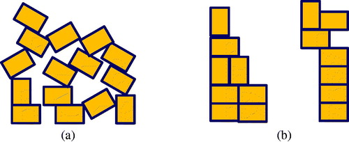
In this paper there are a range of networks examined in terms of the structural complexity. Different moments will be computed for each network. It is a logical question if entropy could be revealing as a measure of complexity. If this is the case, then entropy should increase with the number of components.

4. Computing the systemic moments of exponential-pdf networks

Computing the mean from a structure function was described with Equation (5)(5) $$\mathit{mttf}=\overline{t}=\underset{-\mathrm{\infty }}{\overset{\mathrm{\infty }}{\int }}tf\mathrm{d}t=\underset{0}{\overset{\mathrm{\infty }}{\int }}{R}_{T}dt=\underset{0}{\overset{\mathrm{\infty }}{\int }}{e}^{-\left({\lambda }_A+{\lambda }_B\right)t}dt=\frac{1}{\left({\lambda }_A+{\lambda }_B\right)}$$(5) and the standard deviation is (18). (18) $$\begin{array}{cc}\sigma =\sqrt{\overline{t^2}-{\overline{t}}^2}& \mathrm{w}\mathrm{ith} \mathrm{mean}-\mathrm{square} \end{array}\overline{t^2}=\underset{-\mathrm{\infty }}{\overset{\mathrm{\infty }}{\int }}{t}^{2}fdt$$(18)

The reader will note the mathematical grammar distinguishing

There is not a well-known short-cut formula for the mean-square, so this is often computed from the structure density $f=-\frac{dR}{dt}$ literally using (18). However, the practicing engineer doing that calculation soon sees a pattern, which is very clear in terms of R-kets.

From the appended Table A2 (R-kets) there are some obvious patterns. There is not a term for $x^0$ in these vectors, because the basic ‘building block’ is a single block corresponding to at least a power $x^1.$ From (11) it is immediately apparent that there is an assumption of 100% reliability at time zero. In R-ket form this means the coefficients of any network must sum to unity. However, because these are not probability density vectors, they are not of unit length. Any real-world system that is expressed as a combination of parts (n-vector) can be expanded in terms of the R-kets of the same degree (the state space is spanned).

The last coefficient of any R-ket, the rightmost term is ±1 which is hereafter called the ‘parity’ of a network. Consider, for explaining this, the networks $S_1,\mathrm{ }P,\mathrm{ }{P}_3,\mathrm{ }{P}_4,P_5$ as shown on Table 1.

Table 1. R-kets of ‘pure’ parallel networks with n = 1 to 5 components.

$S_1$	1
$P$	2	−1
$P_3$	3	−3	1
$P_4$	4	−6	4	−1
$P_5$	5	−10	10	−5	1

Each additional parallel element introduces a factor −1. This is not seen for the series networks $S_1,\mathrm{ }S,\mathrm{ }{S}_3,\mathrm{ }{S}_4.$ Apparently, the parity is an indicator of parallelisation. The same is seen starting from any network and considering a similar network with ‘one extra’ parallel sub-net.

The single block network labelled S₁ here is not really a series or parallel permutation but fits the pattern rather like hydrogen fits into the modern periodic table of elements.

The first few coefficients in any R-ket, up until a zero or negative number is reached, describes the number of tie sets of that order. For example, $\mathit{SPPSP}$ is a six-block network with $P$ in series with $\mathit{PSP}:$

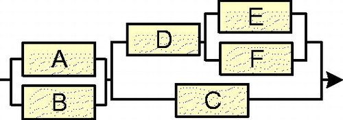
On Figure 5 there are visibly three parallel pairs within the structure of the network explaining its negative parity, even though it is a series of two sub-nets when formulating the structure function. The network/state $\mathit{SPPSP}$ has two second order tie paths and three third order tie paths.

Figure 5. The SPPSP $|0,2,3,-8,5,-1\mathrm{〉}$ network, n = 6, arbitrarily selected as example.

As described under Equation (13)(13) $$\mathit{mttf}=\frac{1}{{\lambda }_A+{\lambda }_B}+\frac{1}{{\lambda }_A+{\lambda }_C}-\frac{1}{{\lambda }_A+{\lambda }_B+{\lambda }_C}$$(13) the R-ket can be processed to obtain the density function in vector form. Keeping to the arbitrarily chosen example $SP(\mathit{PSP})$ the R-ket and f-ket can be found as (16)(14) $$t_{\mathit{maintenance}}\approx \frac{\mathit{mttf}}{20}$$(14) by expanding the R-ket, differentiating, and then reformulating as a vector. (19) $$\begin{array}{c}R=\mathrm{\mid }0,2,3,-8,5,-1\mathrm{〉}\\ R=2e^{-2\mathrm{\lambda }t}+3e^{-3\mathrm{\lambda }t}-8e^{-4\mathrm{\lambda }t}+5e^{-5\mathrm{\lambda }t}-e^{-6\mathrm{\lambda }t}\end{array}$$(19) (20) $$f=-\frac{dR}{dt}=\lambda \mathrm{\mid }0,4,9,-32,25,-6\mathrm{〉}$$(20)

This calculation to obtain (20)(20) $$f=-\frac{dR}{dt}=\lambda \mathrm{\mid }0,4,9,-32,25,-6\mathrm{〉}$$(20) is significantly faster as a vector maths problem. Consider that a vector is converted into a new vector by the application of a matrix operator. In this example the matrix operator represents differentiation acting upon the R-ket column vector. (21) $$\mathrm{\lambda }\left(\begin{array}{cc}\begin{array}{ccc}1& 0& 0\\ 0& 2& 0\\ 0& 0& 3\end{array}& \begin{array}{ccc}0& 0& 0\\ 0& 0& 0\\ 0& 0& 0\end{array}\\ \begin{array}{ccc}0& 0& 0\\ 0& 0& 0\\ 0& 0& 0\end{array}& \begin{array}{ccc}4& 0& 0\\ 0& 5& 0\\ 0& 0& 6\end{array}\end{array}\right)\left(\begin{array}{c}\begin{array}{c}\mathrm{ }0\\ \mathrm{ }2\\ \mathrm{ }3\end{array}\\ \begin{array}{c}-8\\ \mathrm{ }5\\ -1\end{array}\end{array}\right)=\mathrm{\lambda }\left(\begin{array}{c}\begin{array}{c}\mathrm{ }0\\ \mathrm{ }4\\ \mathrm{ }9\end{array}\\ \begin{array}{c}-32\\ \mathrm{ }25\\ -6\end{array}\end{array}\right)$$(21)

The operator here is a diagonal n × n matrix containing the first n integers. This is hereafter denoted ‘Z’ as in Equation (22)(22) $$\begin{array}{cc}Z=\left(\begin{array}{cc}\begin{array}{cc}1& 0\\ 0& 2\end{array}& \begin{array}{cc}\dots & 0\\ \dots & 0\end{array}\\ \begin{array}{cc}⋮& ⋮\\ 0& 0\end{array}& \begin{array}{cc}\ddots & ⋮\\ \dots & n\end{array}\end{array}\right)& Z^{-1}=\left(\begin{array}{cc}\begin{array}{cc}1& 0\\ 0& \frac{1}{2}\end{array}& \begin{array}{cc}\dots & 0\\ \dots & 0\end{array}\\ \begin{array}{cc}⋮& ⋮\\ 0& 0\end{array}& \begin{array}{cc}\ddots & ⋮\\ \dots & \frac{1}{n}\end{array}\end{array}\right)\end{array}$$(22) . The matrix has the Natural numbers as eigenvalues and the eigenvectors are the cartesian orthonormal basis. Using this definition, it is found $f=\lambda ZR$ and $R=\frac{1}{\lambda }{Z}^{-1}f.$ (22) $$\begin{array}{cc}Z=\left(\begin{array}{cc}\begin{array}{cc}1& 0\\ 0& 2\end{array}& \begin{array}{cc}\dots & 0\\ \dots & 0\end{array}\\ \begin{array}{cc}⋮& ⋮\\ 0& 0\end{array}& \begin{array}{cc}\ddots & ⋮\\ \dots & n\end{array}\end{array}\right)& Z^{-1}=\left(\begin{array}{cc}\begin{array}{cc}1& 0\\ 0& \frac{1}{2}\end{array}& \begin{array}{cc}\dots & 0\\ \dots & 0\end{array}\\ \begin{array}{cc}⋮& ⋮\\ 0& 0\end{array}& \begin{array}{cc}\ddots & ⋮\\ \dots & \frac{1}{n}\end{array}\end{array}\right)\end{array}$$(22)

It is also useful at this point to introduce a unit row-vector $\overline{1}=\mathrm{⟨}1,\mathrm{ }1,\mathrm{ }1,\mathrm{ }\dots .,\mathrm{ }1|,$ which has the effect of summing diagonal elements of such a matrix when applied as a scalar product. (23) $$\begin{array}{ccc}\overline{t}=⟨\mathrm{⟨}|1|{\lambda }^{-1}{Z}^{-1}R\mathrm{〉}⟩& \overline{t^2}=2⟨\mathrm{⟨}|1|{\lambda }^{-2}{Z}^{-2}R\mathrm{〉}⟩& \sigma ={\lambda }^{-1}\sqrt{\overline{t^2}-{\left(\overline{t}\right)}^2}\end{array}$$(23)

Using the above example $R=\mathrm{\mid }0,2,3,-8,5,-1\mathrm{〉}$ it is found $\overline{t}=\frac{5}{6\lambda },$ $\overline{t^2}=\frac{91}{90{\lambda }^2}$ and $\sigma =\frac{1}{6\lambda }\sqrt{\frac{57}{5}}\approx \frac{0.563}{\lambda }.$ In this formulation the computation of moments from structure function does not even require exponential expressions. Appended Table A3 gives the mean and standard deviations for the configurations on appended Tables A1 and A2 and entropy as explained below. To be precise the moments are of the form $\overline{t}=\frac{a}{\lambda },$ $\sigma =\frac{b}{\lambda }$ where a and b are the ‘mean parameter’ and ‘standard deviation parameter’ given on the tables. This parameter is the single value that identifies the distinct networks.

Table 2. Series upgrading effects on network properties/moments.

Configuration	R-ket						ΣS	Degeneracy, Ω/ε	o	λ*mttf	λσ
S1	1						1	1	1	1	2.7183
S	0	1					2	2	2	0.5	1.36
S3	0	0	1				3	6	3	0.3333	0.906
S4	0	0	0	1			4	24	4	0.25	0.68
S5	0	0	0	0	1		5	120	5	0.2	0.544

5. Systemic entropy and quantum numbers

The mathematical definition of entropy used in this paper is the common one from thermodynamics and information theory (Guenault, 2007). (24) $$S=-\underset{-\mathrm{\infty }}{\overset{\mathrm{\infty }}{\int }}\mathit{fln}\left(f\right)dt$$(24)

For example, state/network $P_3$ on Figure 3 has R-ket $\mathrm{\mid }3,-3,1\mathrm{〉}$ and density function $f\left(t\right)=3{\lambda e}^{-\lambda t}-6\lambda e^{-2\lambda t}+3\lambda e^{-3\lambda t}=3\lambda x{\left(1-x\right)}^2$ where $x=e^{-\lambda t}.$ It is convenient to change the variable of integration $dx=-\lambda \mathit{xdt}$ and use $1-x=y$ for the final integral. (25) $$S=-\underset{-\mathrm{\infty }}{\overset{\mathrm{\infty }}{\int }}f\left[ln\left(3\lambda \right)+ln\left(x\right)+2ln\left(1-x\right)\right]dt=ln\left(3.437/\lambda \right)$$(25)

The logarithm in (24)(24) $$S=-\underset{-\mathrm{\infty }}{\overset{\mathrm{\infty }}{\int }}\mathit{fln}\left(f\right)dt$$(24) separates the factors of the density function to give a series of simpler integrals (25)(25) $$S=-\underset{-\mathrm{\infty }}{\overset{\mathrm{\infty }}{\int }}f\left[ln\left(3\lambda \right)+ln\left(x\right)+2ln\left(1-x\right)\right]dt=ln\left(3.437/\lambda \right)$$(25) . A couple of standard integrals (26)(24) $$S=-\underset{-\mathrm{\infty }}{\overset{\mathrm{\infty }}{\int }}\mathit{fln}\left(f\right)dt$$(24) resolves many of the calculations, but for irreducible quadratic factors a numerical integration has been used in this paper. (26) $$\begin{array}{cc}{I}_n=\underset{0}{\overset{\infty }{\int }}{t}^n{e}^{-\lambda t}dt=\frac{n!}{{\lambda }^n}& I_n=\underset{0}{\overset{1}{\int }}{z}^{n}ln\left(z\right)dz=\frac{-1}{{\left(n+1\right)}^2}\end{array}$$(26)

The result (25)(25) $$S=-\underset{-\mathrm{\infty }}{\overset{\mathrm{\infty }}{\int }}f\left[ln\left(3\lambda \right)+ln\left(x\right)+2ln\left(1-x\right)\right]dt=ln\left(3.437/\lambda \right)$$(25) is of the form $S=ln\left(c/\lambda \right)$ and ‘c’ is the entropy parameter on Table A3 that identifies the network uniquely. The final appended Table A4 again lists these ‘states’ alongside the number ‘n’ of components and the number of complex pairs of roots corresponding to Table A3. The three ‘index summation’ columns refer to the number of series ‘S’ and parallel ‘P’ letters in the label/name of the state as measures of how the state is constructed internally. Thus $P_3{S}^3$ is short for $P_3{S}_2{S}_2{S}_2$ for which $\sum P=3,$ $\sum S=6$ and $\mathrm{\Sigma }=\sum P+\sum S=9.$

The next three columns of Table A4 refer to the permutations of labellings that can be applied to a given state in analogy to statistical physics. For example, on configuration SP, the three boxes can be labelled a, b, c. There are six permutations of the letters alone: abc, acb, bac, bca, cab, cba this number is labelled Ω. If we assign components reliabilities $R_A=0.9,$ $R_B=0.8,$ $R_C=0.7$7 then for these six micro-states there are only 3 distinct values for total system reliability, and entropy (described as energy state on the table). Systemically there would only be one energy state. The number of micro-states with the same entropy is the degeneracy.

The final column of Table A4 is called ‘tie order’ and refers to the R-ket representation in comparison to the tie sets of the network/state. For example, PS has two second degree/order tie paths. The R-ket is $\mathrm{\mid }0,2,-1\mathrm{〉}$ with the ‘0, 2’ expressing that there are zero first order tie paths and 2 second order tie paths. The parity bit ‘−1’ does not reveal any tie paths. In this example the tie paths were given in the first two numbers of the vector, so the tie-order was recorded as 2. A canonical Boolean structure function could also be used, but this confuses the addition ‘+’ operator with the ‘OR’ operator and can lead to drastically erroneous estimates in risk assessment.

Whilst these characteristic values of the ‘states’ are not the same as the quantum numbers used to describe electronic configurations of atoms, the correlation of these numbers with the moments is examined below to look for any obvious ‘periodicity’.

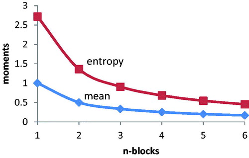
The data from Tables A3 and A4 were used to plot the graphs below to establish the two main aims of this paper; firstly to examine entropy as a moment by comparing it to the more usual mean and standard deviation, and secondly to examine the entropy of the set of states for any apparent trends using the broadly named quantum numbers above.

Table 3. Parallel upgrading effects on network mean/moment λ*mttf.

S1	P	P3	P4	P5	P6
2.718	3.69	4.06	4.25	4.37	4.44

Table 4. ‘Progressive parallelisation’ effects on network mean/moment λ*mttf.

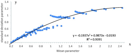
On Figure 6 it is seen that the standard deviation is 94% correlated with the mean for n = 1 to 6 networks. This means that one can often be used to predict the other, introducing only a small error. The same cannot be said for non-systemic networks. The upper limits of the spread of ‘dots’ on Figure 6 correspond to networks that are purely series and purely parallel combinations. There is also a visible a band-structure with gaps on Figure 6. The points for a given number of blocks are spread along the entire length of the best fit line and the gaps would disappear if larger numbers of blocks are introduced. The bands correspond to ‘upgrading’ described below.

Figure 6. Comparing the systemic mean and standard deviation of n < 7 exponential reliability SP-networks.

Figure 7 looks like a better correlated form of Figure 6. This can be understood because entropy involves an integration over a logarithm. Rather like plotting experimental data on logarithmic axis improves apparent correlations. Comparing Figures 6 and 7 there does not seem to be any amazing benefit for the work of computing the more complicated type of moment. Figure 8 compares standard deviation to entropy

Figure 7. Comparing systemic entropy to systemic mean for n < 7 SP-nets.

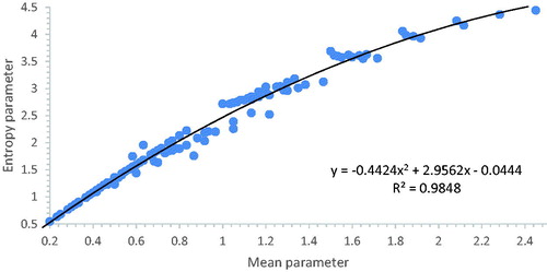
Figure 8. Complexity compared to uncertainty: plot of entropy and standard deviation.

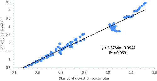
From Figures 6 and 7, it might be expected that Figure 8 would approximate to a straight line with some ‘fine structure’ due to the banding. This is indeed the case and evidently the systemic entropy is roughly 3.4 times the standard deviation for about the first hundred networks on Tables 1–4. The correlation here is 97% and the data for Figure 8 was to only four significant figures accuracy from the tables.

The thermo-dynamical entropy is depicted here as an ensemble average over only a small number of network sub-components. The mathematical extension to very large systems would better exploit the analogy to statistical physics.

6. Systemic upgrading

For want of a better name, this short section is concerned with the systemic entropy changes when a single block is added (or removed) from a network. A limited number of scenarios have been examined for this paper.

6.1. Series upgrading

This is exemplified by the series of states $S_1,$ $S,$ $S_3,$ $S_4,$ etc. It is simply a matter of adding one extra block onto the end of a network. The R-kets, ΣS, degeneracy and moments are given on Table 2.

There is little surprise on Table A1 that the series-sum and order of tie-path increase exactly with the number of blocks in a network, or that the degeneracy is the factorial of the number of blocks for a simple series. The main interest from Table A1 is the effect on the R-ket is to introduce an extra zero on the left because the structure function is ‘enhanced’ as R → xR when an additional reliability is placed in series. This can be mathematically represented by a matrix that transforms the network to the upgraded network in R-ket form. This is simply an (n + 1)×n rectangular matrix composed of a row of zeros and the n-identity matrix. (27) $$U_{\mathit{series}}=\left(\begin{array}{cc}\begin{array}{cc}0& 0\\ 1& 0\end{array}& \begin{array}{cc}\dots & 0\\ \dots & 0\end{array}\\ \begin{array}{cc}0& 1\\ \begin{array}{c}⋮\\ 0\end{array}& \begin{array}{c}⋮\\ 0\end{array}\end{array}& \begin{array}{cc}\dots & 0\\ \begin{array}{c}\ddots \\ \dots \end{array}& \begin{array}{c}⋮\\ 1\end{array}\end{array}\end{array}\right)$$(27)

The mean and standard deviation are the same for simple series using exponential distributions in systemic terms. These moments decrease as 1/n as shown on Figure 9, as the number of blocks is increased. This is a well-known effect for the mean, but decreasing entropy, and thus complexity, for longer network chains is novel.

Figure 9. Moments decrease as 1/n for series upgrading.

6.2. Parallelisation

This is exemplified by the following changes of states: s₁–p–p₃–p₄– etc. which gives a series of vectors $|1〉,$ $|2,-1〉,$ $|3,-3,1〉,$ $[4,-6,4,-1⟩⟩.$ The pattern here is of the form $|a,b,c,d〉$ → $|1+a,b-a,c-b,d-c,-d〉$ which is (28)(28) $$U_{\mathit{parallel}}=\left(\mathrm{ }{\begin{array}{c} 2\\ -1\\ 0\\ 0\\ 0\\ ⋮\\ 0\end{array}\mathrm{ }\begin{array}{c} 1\\ 1\\ -1\\ 0\\ 0\\ ⋮\\ 0\end{array}\mathrm{ }\begin{array}{c} 1\\ 0\\ 1\\ -1\\ 0\\ ⋮\\ 0\end{array}\mathrm{ }\begin{array}{c}\dots \\ \dots \\ \dots \\ \dots \\ \ddots \\ \ddots \\ \dots \end{array}\mathrm{ }\begin{array}{c} 1\\ 0\\ 0\\ 0\\ 0\\ 1\\ -1\end{array}}^{\mathrm{ }}\right)$$(28) in operator form. (28) $$U_{\mathit{parallel}}=\left(\mathrm{ }{\begin{array}{c} 2\\ -1\\ 0\\ 0\\ 0\\ ⋮\\ 0\end{array}\mathrm{ }\begin{array}{c} 1\\ 1\\ -1\\ 0\\ 0\\ ⋮\\ 0\end{array}\mathrm{ }\begin{array}{c} 1\\ 0\\ 1\\ -1\\ 0\\ ⋮\\ 0\end{array}\mathrm{ }\begin{array}{c}\dots \\ \dots \\ \dots \\ \dots \\ \ddots \\ \ddots \\ \dots \end{array}\mathrm{ }\begin{array}{c} 1\\ 0\\ 0\\ 0\\ 0\\ 1\\ -1\end{array}}^{\mathrm{ }}\right)$$(28)

Equation (28)(28) $$U_{\mathit{parallel}}=\left(\mathrm{ }{\begin{array}{c} 2\\ -1\\ 0\\ 0\\ 0\\ ⋮\\ 0\end{array}\mathrm{ }\begin{array}{c} 1\\ 1\\ -1\\ 0\\ 0\\ ⋮\\ 0\end{array}\mathrm{ }\begin{array}{c} 1\\ 0\\ 1\\ -1\\ 0\\ ⋮\\ 0\end{array}\mathrm{ }\begin{array}{c}\dots \\ \dots \\ \dots \\ \dots \\ \ddots \\ \ddots \\ \dots \end{array}\mathrm{ }\begin{array}{c} 1\\ 0\\ 0\\ 0\\ 0\\ 1\\ -1\end{array}}^{\mathrm{ }}\right)$$(28) includes the parallel ‘unit’ $|2,-1〉.$ For example: (29) $$U_{\mathit{Parallel}}{R}_S=\left(\mathrm{ }{\begin{array}{c} 2\\ -1\\ 0\end{array}\mathrm{ }\begin{array}{c} 1\\ 1\\ -1\end{array}\mathrm{ }}^{\mathrm{ }}\right)\left(\begin{array}{c}0\\ 1\end{array}\right)|0,1⟩⟩=R_{PS}$$(29)

The entropy change due to this ‘parallel upgrading’ proceeds as follows:

This is the same pattern as the total system reliability for n-blocks in parallel. This asymptotically tends to a maximum value as 1 − 1/n.

6.3. Parallel expansion

The example state changes for this are: S₁ – SP – S₃P² – S₄P³ giving a series of vectors $|1⟩⟩,$ $|0,2,-1⟩⟩,$ $[0,0,4,-4,1⟩⟩,$ $[0,0,0,8,-12,6,-1⟩⟩.$ The operator is (30)(30) $$U_{\mathit{parallel}}=\left(\mathrm{ }{\begin{array}{c} 0\\ 2\\ -1\\ 0\\ 0\\ ⋮\\ 0\end{array}\mathrm{ }\begin{array}{c} 0\\ 0\\ 2\\ -1\\ 0\\ ⋮\\ 0\end{array}\mathrm{ }\begin{array}{c}0\\ 0\\ 0\\ 2\\ -1\\ ⋮\\ 0\end{array}\mathrm{ }\begin{array}{c}\dots \\ \dots \\ \dots \\ \dots \\ \dots \\ \ddots \\ \ddots \end{array}\mathrm{ }\begin{array}{c} 0\\ 0\\ 0\\ 0\\ 0\\ 2\\ -1\end{array}}^{\mathrm{ }}\right)$$(30) and the pattern is $|a,b,c,d⟩⟩$ → $|0,2a,2b-a,2c-b,2d-c,-d⟩⟩.$ (30) $$U_{\mathit{parallel}}=\left(\mathrm{ }{\begin{array}{c} 0\\ 2\\ -1\\ 0\\ 0\\ ⋮\\ 0\end{array}\mathrm{ }\begin{array}{c} 0\\ 0\\ 2\\ -1\\ 0\\ ⋮\\ 0\end{array}\mathrm{ }\begin{array}{c}0\\ 0\\ 0\\ 2\\ -1\\ ⋮\\ 0\end{array}\mathrm{ }\begin{array}{c}\dots \\ \dots \\ \dots \\ \dots \\ \dots \\ \ddots \\ \ddots \end{array}\mathrm{ }\begin{array}{c} 0\\ 0\\ 0\\ 0\\ 0\\ 2\\ -1\end{array}}^{\mathrm{ }}\right)$$(30)

For example (31) $$U_{\mathit{parallel}}{R}_P=\left(\begin{array}{cc}\begin{array}{c}\begin{array}{c}\mathrm{ }0\\ \mathrm{ }2\end{array}\\ \begin{array}{c}-1\\ 0\end{array}\end{array}& \begin{array}{c}\begin{array}{c}\mathrm{ }0\\ \mathrm{ }0\end{array}\\ \begin{array}{c}2\\ -1\end{array}\end{array}\end{array}\right)\left(\begin{array}{c}2\\ -1\end{array}\right)=\left(\begin{array}{c}\begin{array}{c}0\\ 4\end{array}\\ \begin{array}{c}-4\\ 1\end{array}\end{array}\right)=R_{{SP}^2}$$(31)

The entropies of the sequence S₁ – SP – S₃P² – S₄P³ are 2.72–1.78–1.40– decreasing as 1/n the same as a series of individual blocks.

6.4. Series reduction

By similar choices of networks, the inverse problems can be easily developed. Series reduction, for want of a name, means removing a single component from the end of a chain, opposite to series upgrading. This is again a combination of the identity matrix, this time the operator includes a column rather than a row of zeros. (32) $$U_{\mathit{series}}^{-1}=\left(\begin{array}{c}\begin{array}{cc}\begin{array}{cc}0& 1\\ 0& 0\end{array}& \begin{array}{ccc}0& \dots & 0\\ 1& \dots & 0\end{array}\end{array}\\ \begin{array}{cc}\begin{array}{cc}⋮& ⋮\\ 0& 0\end{array}& \begin{array}{ccc}⋮& \ddots & ⋮\\ 0& \dots & 1\end{array}\end{array}\end{array}\right)$$(32)

For example (33) $$U_{\mathit{series}}^{-1}{R}_{S_4}=\left(\begin{array}{cc}\begin{array}{cc}0& 1\\ 0& 0\\ 0& 0\end{array}& \begin{array}{cc}0& 0\\ 1& 0\\ 0& 1\end{array}\end{array}\right)\left(\begin{array}{c}0\\ 0\\ 0\\ 1\end{array}\right)=R_{S_3}$$(33)

6.5. Progressive parallelisation

This is exemplified by the series of states $S_4,$ $S_{3}P,$ $\mathit{SPS},$ $P{S}_3$ (Figure 10).

Figure 10. The four n = 4 configurations illustrating ‘progressive parallelisation’.

Clearly there are many such patterns to explore in any future study. The operator for this one is yet incompletely specified (33) such that the columns contain 2, −1 save the first, which is to be chosen to simplify the inverse matrices. (34) $$\begin{array}{cc}{U}_{pp,2}=\left(\begin{array}{cc}a& 2\\ b& -1\end{array}\right)& U_{pp,3}=\left(\begin{array}{ccc}a& 1/2& 0\\ b& 3/2& 2\\ c& -1& -1\end{array}\right)\\ & U_{pp,4}=\left(\begin{array}{c}a\\ b\\ c\\ d\end{array}\begin{array}{c} 1\\ -1/2\\ 3/2\\ -1\end{array}\begin{array}{c}0\\ 1/2\\ 3/2\\ -1\end{array}{\begin{array}{c} 0\\ 0\\ 2\\ -1\end{array}}^{}\right)& \end{array}$$(34)

To examine the entropy changes caused by this ‘enhancement’ consider a sequence of states:

This is clearly following the pattern of more and more parallel in a network.

7. Non SP-networks

There are some networks that cannot be Boolean-reduced to combinations of series and parallel parts only. The best known of these is the simplest, the bridge network (Figure 11). (34) $$\begin{array}{cc}\begin{array}{c}T=\left(AB+CD\right)+\left(\mathit{ADE}+\mathit{BCE}\right)\\ -\left(\mathit{BCDE}+\mathit{ACDE}+\mathit{ABDE}+\mathit{ABCE}+\mathit{ABCD}\right)\\ +2A\mathit{BCDE}\end{array}& R_{B_1}=|0,2,2,-5,2〉\end{array}$$(34) (35) $$\begin{array}{ccc}\overline{t}=49/60\lambda & \sigma =\sqrt{41}/12\lambda & s=ln\left(0.3756/\lambda \right)\end{array}$$(35)

Figure 11. The n = 5 bridge configuration $B_1.$

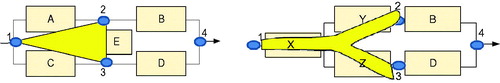
7.1. Transform the network into SP-form

There are two ways widely known to obtain a structure function for non SP-systems. There is an analogy to impedance in electronic circuits. On Figure 12, a triangle is superimposed onto the bridge network, and its equivalent Y-shaped subnetwork is shown (Kennelly, 1899). To complete the analogy, it is a matter of some algebra to obtain {X,Y,Z} and (A,C,E} in terms of each other. (36) $$\begin{array}{cc}X=\frac{AC}{A+C+E}\hspace{1em}& A=\frac{XY+XY+YZ}{Z}\\ Y=\frac{AE}{A+C+E}\hspace{1em}& C=\frac{XY+XY+YZ}{Y}\\ Z=\frac{CE}{A+C+E}\hspace{1em}& E=\frac{XY+XY+YZ}{X}\end{array}$$(36)

Figure 12. The ‘triangle-Y’ transformation.

7.2. Hybridisation

The network is imagined to be a synthesis of two networks: one where the bridge element has failed ($P{S}^2$) and one where the bridge element is 100% reliable ($S{P}^2$). This is denoted here as $S{P}^2\curvearrowright P{S}^2$ and is mathematically achieved from the R-kets as $B_1=xS{P}^2+\left(1-x\right)P{S}^2$ where ‘$x$’ is the reliability of the bridging element. Recall that multiplication by ‘$x$’ previously had the effect of right-shifting the R-ket and inserting an extra zero. (37) $$\begin{array}{c}{B}_1=xS{P}^2+P{S}^2-xP{S}^2\\ =|0,0,4,-4,1〉⟩+|0,2,0,-1,0〉⟩-|0,0,2,0,-1〉⟩\\ =|0,2,2,-5,2〉⟩\end{array}$$(37)

In this way it is a question if any two networks could be bridged together, one superimposed on the other. The reader could try this exhaustively, then rule-out any pre-existing networks such as S₁ $\curvearrowright$ S = SP and note that for any network $A\mathrm{ }\curvearrowright A=A.$ Furthermore, feasible bridges (i.e. Ones that can be drawn) would have a parity of ±2 requiring that appropriate networks to combine should have compatibly opposite parities. This still leaves a number of new networks to rule-out and this paper only suggests that this may possibly be explained in terms of the polynomial roots.

8. Relaxing the exponential assumption

The Weibull distribution (2)(2) $$R=e^{-{\left(t/s\right)}^{\beta }}$$(2) introduces that extra one parameter to complicate everything above in this paper. All the R-kets now need to be pre-multiplied by $\alpha =\frac{\beta }{s}{\left(\frac{t}{s}\right)}^{\beta -1}$ so that, for example, $B_{P{S}^2}=\propto |0,2,0,-1,0〉⟩.$ The moments are found to be (38)(37) $$\begin{array}{c}{B}_1=xS{P}^2+P{S}^2-xP{S}^2\\ =|0,0,4,-4,1〉⟩+|0,2,0,-1,0〉⟩-|0,0,2,0,-1〉⟩\\ =|0,2,2,-5,2〉⟩\end{array}$$(37) (38) $$\begin{array}{cc}\overline{t}=⟨⟨1|z^{-1-\frac{1}{\beta }}|R〉⟩& \overline{t^n}=⟨⟨1|z^{-{\left(1+\frac{1}{\beta }\right)}^n}|R〉⟩\end{array}$$(38)

To apply this method to the systematic (i.e. Not systemic) problem, the coefficients of the vectors would no longer refer to integer powers of ‘x’ and the vectors/matrices would have different lengths. This is beyond the scope of this paper.

9. Discussion

This paper has introduced a labelling system to distinguish SP-networks of arbitrary order, but it requires modification to encompass non SP-networks (hybrids) and cumbersome use of parenthesis appears to be needed for higher order networks. A set of tables was given of the first n = 5 networks and their properties. Non-integer numbers of components are beyond the scope of this paper. Another way to represent the networks, using cartesian vectors, was reviewed and it was found that the standard moments were easily computed from this, along with a series of characterising numbers. The moment ‘systemic entropy’ was compared to systemic means and standard deviations and no real advantage was obtained, save that it is ‘understood’ to represent complexity of a network. Entropy changes with simple changes to the system were explored.

The paper reviewed non SP-networks and how hybridisation is represented in vector form. Finally, the exponential distribution was relaxed to a Weibull distribution and it was found that the vector form was changed only by a multiple.

In conclusion any real system can be understood to be a hybrid, distributed across a range of states. The mean, standard deviation and other moments are measures of system risk. Risk itself is a quantum state of a system/process and there are analogies with statistical physics. The risk manager, armed with this study, can consider how specifying one step of a process into a series of two smaller steps will reduce entropy due to the increase in information given, yet back-up systems increase uncertainty. Furthermore, whilst a system may be designed to precisely represent one network state, the reality will always be a diffusion across different specifications, mainly with variations of clarity of subsystems.

There are many aspects of this work that can be pursued in analogy to statistical physics: amplitude functions, different distributions and distribution moments and quantum numbers, etc. But the future work envisioned is concerned with the fault tree and event tree forms of block diagrams, higher order bridges, Karnaugh graphs and applying the network-entropy to the complexity of buildings for purposes of fire safety evacuation modelling.

Abbreviations
MTTF	=	Mean time to failure
STOP	=	Series-Two-One-Parallel
RAMS	=	reliability, availability, maintainability and safety
R-ket	=	Column vector of the polynomial coefficient representation of systemic reliability structure function

Disclosure statement

No potential conflict of interest was reported by the author(s).

Additional information

Notes on contributors

Tony Lee Graham

Dr Graham is a Senior Lecturer in Fire Engineering. After studying theoretical physics he moved into modelling of fire dynamics. He has been researching fire dynamics for over two decades. He primarily teaches fire dynamics and probabilistic risk assessment and has taught over 150 classes in three countries. His research is within the area of fire and hazards science and is a member of the Centre for Fire and Hazards Science. Tony is a member of Institute of Physics, Energy Institute, Combustion Institute and Institution of Fire Engineers. He is a Chartered Physicist and Engineer and is a Senior Fellow of the Advance Higher Education Academy UK.

Khalid Khan

Dr Khan is currently a Senior Lecturer in Engineering Mathematics in the school of Engineering. He teaches on a range of mathematics modules within the Fire degree programmes and contributes to other mathematics teaching within the School and Faculty. Dr Khan is research active within the Centre for Fire Hazard Studies. Dr Khan’s research interests are in the area of mathematical modelling of system behaviour in a range of applications. His current work focuses on fire suppression using sprinkler systems and on mathematical models of collective motion of self-propelled particles in homogeneous and heterogeneous mediums. Dr Khan has currently over thirty publications and is also a member of two journal review panel boards.

Hamid Reza Nasriani

Dr Nasriani is currently a Senior Lecturer in Oil & Gas Engineering in the school of Engineering. He teaches on a range of oil & gas modules within the Oil & gas degree programme and contributes to other modules teaching within the School of Engineering and School of Management. Dr Nasriani is research active within the area of Numerical modelling, Simulation, Unconventional formations, Hydraulic Fracturing and Clean-up efficiency of Hydraulic Fractures.

Appendix

Configurations/possible system states

This list is NOT exhaustive.

Table A1. List of block networks n = 1 to 6 with SP-names and labelled blocks.

Table A2. List of states and R-kets.

Table A3. ‘Moment factors’ for the configurations on Table A1^a.

Configuration	Mean	SD	Entropy
	λ * mttf	λ *σ	S
S1	1.0000	1.0000	2.718
S	0.5000	0.5000	1.360
P	1.5000	1.1180	3.690
S3	0.3333	0.3333	0.906
P3	1.8333	1.1667	4.060
PS	1.1667	0.9574	2.942
SP	0.6667	0.5774	1.780
S4	0.2500	0.2500	0.680
P4	2.0830	1.1932	4.251
S3P	0.4167	0.3819	1.127
P3S	1.5830	1.0830	3.619
PS3	1.0833	0.9610	2.789
SP3	0.7500	0.6292	1.999
PS^2	0.7500	0.5590	1.847
SPS	0.5833	0.5069	1.557
SP^2	0.9167	0.6292	2.182
PSP	1.2500	0.9465	3.032
S5	0.2000	0.2000	0.544
P5	2.2833	1.2098	4.366
SP4	0.8000	0.6683	2.132
P4S	1.8833	1.1418	3.964
S4P	0.3000	0.2828	0.814
PS4	1.0500	0.9708	2.737
P3S3	1.5333	1.0960	3.597
S3P3	0.4500	0.4113	1.218
S3P^2	0.5333	0.4295	1.401
SP3P	1.0500	0.6652	2.389
SPS3	0.5500	0.4924	1.471
S3PS	0.3833	0.3468	1.034
PS3S	0.6333	0.4910	1.957
P3S^2	1.2833	0.9293	2.967
PSP3	1.3000	0.9469	3.114
P3SP	1.6333	1.0682	3.610
SP3S	0.7000	0.5831	1.859
PS3P	1.1167	0.9500	2.819
SPSP	0.6167	0.5188	1.637
SPS^2	0.4667	0.383	1.227
PSPS	0.8667	0.5972	1.759
PSPS	1.2000	0.9434	2.934
PSPP	1.3833	0.9239	3.070
SPPS	0.7833	0.560	1.892

a Table A3 uses shading to visually distinguish different values of network components. The table is significant in showing trends in the moments as the number of series and parallel sub-systems increases, and that the moments are broadly of equal value within the ‘systemic’

Table A4. Characteristic values for the configurations on Table A1^a.

Configuration	n	Complex pairs	Index summation			Microstates	Energy states	Degeneracy	Tie order
			ΣP	ΣS	Σ	Ω	ε1	Ω/ε	o
S1	1	0	0	1	1	1	1	1	1
S	2	0	0	2	2	2	1	2	2
P		0	2	0	2	2	1	2	1
S3	3	0	0	3	3	6	1	6	3
P3		1	3	0	3	6	1	6	1
PS		0	2	2	4	6	3	2	2
SP		0	2	2	4	6	3	2	2
S4	4	0	0	4	4	24	1	24	4
P4		1	4	0	4	24	1	24	1
S3P		0	2	3	5	24	6	4	3
P3S		1	3	2	5	24	6	4	1
PS3		1	2	3	5	24	4	6	3
SP3		1	3	2	5	24	4	6	2
PSS		0	2	4	6	24	3	8	2
SPS		0	2	4	6	24	12	2	3
SPP		0	4	2	6	24	3	8	2
PSP		1	4	2	6	24	12	2	2
S5	5	0	0	5	5	120	1	120	5
P5		2	5	0	5	120	1	120	1
SP4		1	4	2	6	120	5	24	2
P4S		1	4	2	6	120	10	12	1
S4P		0	2	4	6	120	10	12	4
PS4		1	2	4	6	120	5	24	4
P3S3		2	3	3	6	120	10	12	1
S3P3		1	3	3	6	120	10	12	3
S3PP		0	4	3	7	120	15	8	3
SP3P		1	5	2	7	120	10	12	2
SPS3		1	2	5	7	120	20	6	4
S3PS		0	2	5	7	120	60	2	4
PS3S		1	2	5	7	120	10	12	3
P3SS		1	3	4	7	120	15	8	2
PSP3		1	5	2	7	120	10	12	2
P3SP		1	5	2	7	120	30	4	2
SP3S		1	3	4	7	120	30	4	2
PS3P		2	4	3	7	120	30	4	3
SPSP		1	4	4	8	120	60	2	3
SPSS		0	2	6	8	120	15	8	3
PSSP		1	4	4	8	120	30	4	2
PSPS		2	4	4	8	120	60	2	3
PSPP		1	6	2	8	120	15	8	2
SPPS		0	4	4	8	120	30	4	3

a Table A4 uses shading to visually distinguish different values of network components. The table shows different ways to evaluate the degree of series and parallel within a network; and the number of different ways to draw the same network with equal system reliability. These numbers help to establish a logical sequence in the list of different networks.

MTTF: Mean time to failure; STOP: Series-Two-One-Parallel; RAMS: reliability, availability, maintainability and safety; R-ket: Column vector of the polynomial coefficient representation of systemic reliability structure function

References

- Black, F., & Scholes, M. (1973). The pricing of options and corporate liabilities. Journal of Political Economy, 81(3), 637–654.
- Dirac, P. A. M. (1939). A new notation for quantum mechanics. Mathematical Proceedings of the Cambridge Philosophical Society, 35(3), 416–418.
- Guenault, T. (2007). Statistical physics. Student Physics Series. Springer.
- Kennelly, A. E. (1899). Equivalence of triangles and three-pointed stars in conducting networks. Electrical World and Engineer, 34, 413–414.
- Menezes, R., & Oliveira, Á. (2015). Risk assessment and stock market volatility in the Eurozone: 1986–2014. Journal of Physics: Conference Series, 604, 012014. https://doi.org/10.1088/1742-6596/604/1/012014
- Saleh, J. H., & Marais, K. (2006). Highlights from the early (and pre-) history of reliability engineering. Reliability Engineering & System Safety, 91(2), 249–256. https://doi.org/10.1016/j.ress.2005.01.003
- Sifonte, J. R., & Reyes-Picknell, J. V. (2017). Reliability centered maintenance-reengineered. CRC Press.