Investment Decisions and Depreciation Choices under a Discretionary Tax Depreciation Rule

Abstract

Prior studies have shown limited impact of the US bonus depreciation rules on firm investments during economic downturns. In this article we study the effects of a set of more flexible rules – discretionary tax depreciation (DTD) – introduced in the Netherlands during the 2009–2011 economic crisis. Our simulation results show DTD, which allows firms to accelerate and also to postpone depreciation, to be much more effective than bonus depreciation in reducing the expected value of tax payments, especially in crisis periods. Using a sample of 325 clients of a single office of a Dutch accounting firm, we show that DTD has led to higher investments in assets qualifying for discretionary depreciation for firms that faced the highest marginal tax rate. For other firms, the additional investments crowd out investments in assets that do not qualify for DTD. Our analysis on the actual depreciation choices reveals that firms postpone depreciation when facing losses or loss carry forwards, or to smooth taxable income under the progressive tax system. Our results suggest that a fiscal policy that permits firms to postpone depreciation, as well as to accelerate, may stimulate investment.

1. Introduction

Often during an economic downturn firms lower their level of investment. Governments may launch initiatives to try to counter this. One possibility is for them to introduce more favorable business tax regulations, such as the bonus depreciation program initiated by the US Congress following September 2001. Under that program firms were permitted to immediately depreciate (expense) an additional 30% of qualifying investments (in 2002) which was increased to 50% in 2003. In this way, they could defer tax payments to later periods to decrease the present value of their tax payments and improve their current cash position. Klemm (2010) calls for studies that shed more light on the impact of such incentive systems. A number of studies have analyzed whether the bonus depreciation program did in fact lead to higher levels of investment. House and Shapiro (2008) found a small positive effect of bonus depreciation on the level of investment,¹ while the study of Hulse and Livingstone (2010) yielded mixed findings. Other studies suggested reasons for why such programs were not more successful. Edgerton (2010) argues that since such tax incentive programs are initiated when firms have low cash flows, they simply are unable to use the additional tax benefits. Hanlon and Heitzman (2010) caution that although bonus depreciation might lead to higher investments in categories covered by the program, there is a risk of crowding out investments in other assets, as illustrated by Huston (2010). Finally, Knittel (2007) points out that during times when such programs are in effect many firms may have low profits or even loss carryovers, in which case the option to accelerate depreciation is of little value. Taken together, the question of whether the bonus depreciation rule was effective remains by and large unanswered.

In our study, we examine the effects of a temporary regulation instituted by the Dutch government to stimulate investment during the financial crisis of 2009–2011. A discretionary tax depreciation (DTD) rule was introduced that applied to specific types of assets. Under this rule, firms could choose to depreciate covered assets almost completely flexibly, the only constraint being that in the year of investment depreciation was restricted to a maximum of 50% of the depreciable amount. So, firms could take bonus depreciation, but could also choose not to depreciate in the current year in favor of realizing the tax benefits later. In other words, the program introduced in the Netherlands offered firms the possibility of depreciating a higher percentage immediately, like the US bonus depreciation program, but unlike what was offered by the Internal Revenue Services (IRS), firms also had the option of depreciating at a less than normal level (e.g. determined by straight line depreciation) in favor of shifting depreciation deductions to later years in which they were allowed to depreciate at any rate. The option to depreciate less than normal meant that firms incurring losses, or that were making little or no profit, could benefit by banking additional depreciation for use in the future. Adding bonus depreciation to the loss carryforward is not comparable as loss carryovers may expire unused, but depreciation may under this rule be postponed forever (see also Aarbu & MacKie-Mason, 2003, p. 230). Not depreciating at all implies that a higher percentage of the loss carryover can be used. In fact the reported valuation allowances in the US suggest that many deferred tax assets (among which are loss carryforwards) will in the end not yield any tax benefits and expire unused (Poterba, Rao, & Seidman, 2011). We therefore expect that the flexibility of this regulation makes it effective in stimulating investment even at times when firms are less profitable and have low effective tax rates.

Using Monte Carlo simulations, we show that indeed in crisis situations – scenarios where income is highly uncertain and low in the short term – the DTD rule still yields a large increase of the expected present value of tax deductions (EPTD), whereas bonus depreciation has, in line with criticism explained above, very limited effects. To analyze (i) the effects on firm investments and (ii) the use of the discretion allowed, we were granted access to data on 325 small and mainly agricultural Dutch firms from 2009 through 2011, the three years the Netherlands had in place the DTD rule. Our population consists of all of the clients of the largest office of a Dutch accounting firm.

We have two research questions. First, whether the DTD program in the Netherlands was successful in stimulating investment – success being an increase in investments over the expected level taking into account possible crowding out effects with respect to investments in assets not covered by the program. In order to control for selection effects, we analyze what types of firms were more likely to invest in qualifying assets. Second, we examine how firms used the flexibility offered under the program. We analyze which variables influenced tax depreciation choices (e.g. loss carryforwards, marginal tax rates, firm profits), and how firms allocated depreciation charges over time under the progressive tax system of the Netherlands.

We find that the 2009–2011 Dutch DTD rule was indeed to some extent successful in stimulating investment. In general, compared to expected levels of investment based on firm level investment determinants and controlling for whether the firm invested, there was no greater level of investment for firms that invested in those assets that qualify for DTD. However, for firms that faced the highest marginal tax rate, there was a greater level of investment, which suggests that these greater investments were either accelerated or newly-planned. In general, we find evidence that firms’ investments in qualifying assets crowded out investments in assets that did not qualify for DTD, but in line with the earlier result, this effect is not found for firms with the highest marginal tax rate. This result is robust when we control for self-selection.

In the progressive tax system in our setting marginal tax rates explain a significant amount of the variation in utilization of depreciation discretion; when firms incur losses or have a tax loss carryforward they do postpone depreciation charges. We also find evidence that under the progressive tax system firms use depreciation to smooth taxable income over a number of years, which has been shown to be an optimal strategy (Wielhouwer, De Waegenaere, & Kort, 2002). Firms that would move into a lower tax bracket were they to depreciate maximally on average forego current tax savings and thus smooth taxable income. We find that especially firms with more cash and less risk of having lower marginal tax rates in future years smooth taxable income. We note that, although flexible depreciation schemes are often argued to affect only the timing of tax payments (Klemm, 2010), in non-linear tax systems it could affect the amount of tax payments as well.

Our study adds to the literature in several ways. First, we show that DTD may indeed overcome some of the limitations of bonus depreciation in times of crisis, and provide evidence of some positive effects of this fiscal policy on the level of investment. Second, we explicitly investigate the possible crowding out effects. Previous studies on the effectiveness of bonus depreciation have focused on the overall effects on investment at either the level of the firm (Hulse & Livingstone, 2010) or at more macro levels (House & Shapiro, 2008), the only exception being, to our knowledge, Huston (2010) who hand-collected data on the nature of the assets for a sample of 104 firms. Our data, like that of Huston, include investments in all assets together with a distinction whether the assets qualified for DTD. This allows us to investigate potential crowding out effects in more detail. Third, we study the interaction between facing a high marginal tax rate and investing in assets with accelerated depreciation possibilities and in this way show that the effectiveness of these regulations are firm specific. This indicates that distributional concerns should be taken into account when considering such policies to stimulate investments. Fourth, our data allow us to study how flexibility in taking depreciation is actually used by firms. Knittel (2007) showed that a considerable share of small firms do not take advantage of the benefits offered by bonus depreciation, and Cohen and Cummins (2006) that only around 55% of them do actually use it. In studying the underutilization of tax depreciation by Norwegian firms, Aarbu and MacKie-Mason (2003) found that underutilization decreased after decoupling tax and financial accounting. Our study provides insight on why and when firms choose not to depreciate to the maximum extent permitted. We provide evidence that firms are willing under a progressive tax system to forego current tax savings in order to reduce their future tax burden, especially if their current cash position allows such postponement.

Taken together, these findings suggest that DTD, that is, a more flexible system that, rather than allowing only accelerated depreciation, gives firms the option to postpone depreciation in combination with the possibility of depreciating at an accelerated rate in later years, can indeed be effective in stimulating (i.e. increasing or accelerating) investment, especially under a progressive tax system. Our results show that flexibility is indeed used in both directions.

In the next section we review related literature and develop our hypotheses. In Section 3 we explain the DTD rule instituted in the Netherlands. In Section 4 we provide Monte Carlo simulation results to compare the effects of DTD with those of bonus depreciation. In the final three sections we describe our sample, data and models; report the results of our empirical analysis; and conclude.

2. Literature Review and Hypotheses

2.1. Does Flexibility in Tax Depreciation Stimulate Investments?

The literature on the effects of tax depreciation on investment goes back to at least Hall and Jorgenson (1967) who measured the effect of tax depreciation on the cost of investments and empirically investigated the relationship between tax policy and investment in capital. A number of studies since have analyzed effects on the level of investment of temporary regulations that allow increases in depreciation rates. For instance, for two years following 11 September 2001 US firms were able to take advantage of bonus depreciation. In 2002 the regulations allowed them to take an additional 30% of the investment in the year of investment. This bonus depreciation rate was increased to 50% in 2003. The remainder of the investment was to be depreciated in the normal way. Similar bonus depreciation rules are in place since 2008. Cohen, Hansen, and Hassett (2002) provide a theoretical basis for the effect of such rules: they decrease a firm’s cost of capital and hence should result in higher investment. Several empirical studies analyze whether extended depreciation possibilities help to maintain investment levels.

Hulse and Livingstone (2010) use 1990–2006 Compustat data to attempt to establish whether the level of investment was actually higher than expected in 2002 and 2003 in the USA. They find little effect. The level was not significantly higher in 2002 and even significantly lower in 2003. The level was only significantly higher at the end of 2001, when firms anticipated retroactive implementation of bonus depreciation. House and Shapiro (2008) also find using data from the Bureau of Economic Analysis that most of the positive effects on the level of investment took place in the final quarter of 2001. Cohen and Cummins (2006) conclude that bonus depreciation was not effective. Eichfelder and Schneider (2014) study a bonus depreciation possibility for investments in Eastern Germany after the reunification. They find a statistically significant increase in investments in the region during the program, but document that this is partially driven by speeding up investments as there was a significant decrease in investments after the regulation expired.

Edgerton’s (2010) analysis of the potential stimulating effect of temporary bonus depreciations shows that tax asymmetry, that is, only firms with positive taxable income pay tax, leads to a 4% lower effectiveness of bonus depreciation, and also that declines in cash flows decrease effectiveness by 24%. This means that temporary bonus depreciation regulations are actually least effective when they are most needed, that is during periods of economic downturn. Edgerton’s (2010) results are especially important when considering the bonus depreciation rules instituted by the USA which were applicable only in the year in which the investment was made, rendering the opportunity of little value for firms not subject to tax in that year and for those with a loss carryforward. In addition to this, Hanlon and Heitzman (2010) argue that investments that are made as the result of such bonus depreciation programs are likely to crowd out other investments. This is supported by the results of Huston (2010), who shows for a sample of 104 firms that investments in assets covered by the program increased, while investments in other assets decreased. Finally, Edgerton (2012) suggests that the effectiveness of tax depreciation incentives may be limited because of the tendency of managers to focus on accounting earnings which are not affected by tax depreciation (see also Shackelford, Slemrod, & Sallee, 2011). Indeed, when surveyed, managers of large firms indicated that for them tax depreciation does not carry a great deal of weight when they are making investment decisions (Porcano, 1984, 1987; Rose & O’Neil, 1985).

The 2009–2011 DTD program in the Netherlands offered firms the opportunity to take additional depreciation not only in the year an investment is made but also in later years. Such flexibility makes DTD more effective during a downturn as firms are able to realize the tax benefit in the future when profits are expected to be higher. Moreover, under the rules of the Dutch program, firms could postpone depreciation, so that these depreciation charges are not added to the loss carryforward. They could completely flexibly depreciate in later profitable years or use depreciation to avoid moving into a higher tax bracket. As we will see from the simulation results reported in Section 4, such flexibility can have large effects on the expected present value of tax payments. Our sample consists of non-listed firms only, in which managerial focus on accounting earnings may be much less (Kosi & Valentincic, 2013). All and all, we expect the flexible depreciation rules that we consider to stimulate investment. Moreover, the higher the tax rate a firm faces, the more benefits the flexible depreciation rule yields, relatively. So we expect the stimulating effect to be strongest for firms with the highest marginal tax rate. There is however no reason to expect that there is no partial crowding out of investments that do not qualify for discretionary depreciation as cash may be limited. This leads to the following hypotheses.

Hypothesis 1a: The discretionary tax depreciation program stimulated overall firm investments.

Hypothesis 1b: The discretionary tax depreciation program stimulated overall firm investments more when a firm’s marginal tax rate is high.

Hypothesis 1c: Investments in assets qualifying for the program partially crowd out other investments.

2.2. How is Flexibility in Tax Depreciation Actually Used?

The empirical literature on utilization of tax depreciation flexibility is limited, a notable exception being Aarbu and MacKie-Mason (2003) who examined why some Norwegian firms forwent tax depreciation deductions. Based on a sample of approximately 16,800 firm-years collected from government agency Statistics Norway, they found that during years when uniform reporting of tax and book depreciation was required around 40% of firms underutilized by 10–20% on average the tax depreciation options available. In 1992 when depreciation rules were changed and separate reporting was allowed, the percentage of firms underutilizing the tax depreciation options was cut in half, and of the 20% of firms still not taking full advantage, average underutilization fell to 9%. Underutilization was higher among firms with loss carryovers, those that had low performance, and those for which tax compliance costs were high due to different accounting and tax systems. They found that the impact of low performance on underutilization was greater for smaller firms than for medium sized and large firms. The explanation provided for this result is that smaller firms more likely use the same reporting conventions for both tax and accounting reports in order to reduce administrative costs. In line with this thinking, we expect that utilization of flexibility is positively associated with the marginal tax savings of depreciation, because deviating from the normal depreciation scheme imposes an additional administrative burden, that should be offset by the benefits of reduced tax payments. This is more likely when facing a high marginal tax rate. A lower marginal tax rate yields lower benefits of more accelerated depreciation. Similarly, Aarbu and MacKie-Mason (2003, p. 230) argue that ‘Tax loss carryforwards compete with tax deductions. Loss carryforwards expire, while depreciation can be postponed forever’, so that we expect firms to postpone depreciation when they face losses or have loss carryforwards.

The operations research and accounting literature has studied how specific firm characteristics affect the choice of tax depreciation rules. Major effects are: the time value of money (Wakeman, 1980), income uncertainty (Berg, De Waegenaere, & Wielhouwer, 2001; De Waegenaere & Wielhouwer, 2002), tax loss carryovers (Kulp & Hartman, 2011) and the progressivity of the tax system (Wielhouwer et al., 2002). Most of this literature assumes that choices have to be set ex ante and cannot be changed.² The intuition behind the importance of income uncertainty is that depreciation charges may exceed cash flows, yielding a loss in tax deductions (or a loss carryover, which under the tax code of many countries cannot be used unlimitedly to offset future taxable profits). However, under DTD, depreciation charges can be determined ex post. Hence, firms know precisely their earnings and taxable income so that they can avert foregoing tax deductions as depreciation can be increased or decreased depending on actual income.

Berg et al. (2001) and Wielhouwer et al. (2002) have shown that it is optimal for firms to smooth their taxable income under a progressive tax system. In such a system, DTD may thus affect not only the timing but also the amount of tax payments. When firms might face a higher marginal tax rate in the future, they have incentives not to use all the flexibility available, which means that firms with lower marginal tax rates, having reason to believe that they might face higher rates in the future, are likely to have lower utilization rates. Most of the firms in our sample are subject to a highly progressive income tax system. This allows us to investigate whether firms will forego current tax benefits when there is the possibility that they may face a higher marginal tax rate the following year. We test whether firms save their right to tax deductions for the future by analyzing utilization of firms that are able to move into a lower tax bracket by depreciating maximally. We expect that when they are approaching the low end of a tax bracket, for instance they are nearing the point where they would move out of the 52% bracket to the 42% one, they depreciate less, because the option to depreciate might be of more value later.

In sum, we expect utilization of depreciation to increase with the marginal tax rate, and to decrease when there is a loss carryforward or a loss in the current year. We also expect that firms postpone some depreciation charges when full utilization would make them fall into a lower tax bracket. This leads to the following hypotheses regarding the utilization rate of tax depreciation, that is, the actual fraction used of the totally permitted tax depreciation.

Hypothesis 2a: Firms subject to a higher marginal tax rate have a higher utilization rate.

Hypothesis 2b: Firms with a loss carryforward or a loss in the current year have a lower utilization rate.

Hypothesis 2c: Firms that would be in a lower tax bracket with full utilization have a lower utilization rate.

3. DTD as Applied in the Netherlands

From 2009 to 2011 firms in the Netherlands were able to depreciate up to 50% of the total depreciable amount of new investments in the investment year and the residual tax base completely flexible in the following years.³ For example, if a firm chose to depreciate in the investment year only 30% then in the second year the remaining 70% could be depreciated. Clearly this is more flexible than what was possible under the bonus depreciation system offered in the USA, as it meant that Dutch firms that had no tax to pay, because they carried forward a loss or had a loss in the current year, could save depreciation deductions for later years. Together with the introduction of this DTD rule in The Netherlands, the carryback possibility was extended from one to three years, but under the condition that when the carryback option was used, the carryforward period was reduced from nine to six years. The Dutch applied the rule to 2009, then extended it to 2010, and then again to 2011. Prior studies have found that extending an option step-by-step in this way prompts firms to make timely decisions about making additional investments, something that they might not do if it were known from the beginning that an option would be available in subsequent years, an outcome which dilutes the effectiveness of tax rules (Knittel, 2007).

We will refer from this point to assets that qualified under the DTD rules in place in the Netherlands from 2009 to 2011 as DTD-assets, and to investment in such assets as DTD-investment. Some examples of such investments are new computers, machinery, and trucks. DTD was only not permitted on assets to be rented to third parties, used assets, intangible assets, land, buildings, roads and tracks, cars and motorcycles, or animals. We elaborate on the details related to our sample in Section 5.1.

4. Benefits of Bonus Depreciation and Discretionary Depreciation

In order to compare the benefits of discretionary depreciation to those of bonus depreciation, we estimate the EPTD using Monte Carlo simulation under different expectation scenarios of the future. Temporary flexibility in tax depreciation rules can stimulate investment by increasing the EPTD so that the net present value of an investment is increased. Hall and Jorgenson (1967) assumed positive taxable income in calculating the EPTD under different tax depreciation rules. We, on the other hand, estimate the EPTD assuming uncertain, and thus possibly negative, income where, under bonus depreciation rules and under DTD rules, depreciation charges may be set ex post depending on income realization.

For our simulation we assume that future income before taxes is normally distributed. We estimate the EPTD based on the average of 25,000 simulations. Under bonus depreciation firms may take an additional depreciation of 30% or 50% in year one, and under DTD we model the Dutch rule, which limits depreciation in year one to 50% of the investment. We consider a period of five years, and compare tax payments to a benchmark of straight line depreciation, so that under the two bonus depreciation rules maximum depreciation is 50% and 70%, respectively.⁴ To shed more light on the possible effects of these rules, we also compare the results to the EPTD under the most flexible rule possible, that is, immediate expensing (full depreciation in the first year) is permitted together with unlimited loss carryforward. For the other rules we assume however that carrying forward losses is not permitted.⁵

We calculate the EPTD when the firm optimally plans its tax depreciation, meaning that because depreciation charges are set ex post, depreciation is set equal to the maximum allowed when income exceeds that maximum. Otherwise, total income is depreciated to make taxable income equal to zero, unless the income is lower than the minimum depreciation allowed; in that case the minimum depreciation charge is taken, which means that a part of it is lost for tax saving purposes. That minimum is 20% of the investment in year one under bonus depreciation as depreciating less than the benchmark of straight line (SL) depreciation is not allowed. Under DTD the minimum is zero. Thus, both bonus depreciation and DTD are options under which a firm is never worse off than under SL depreciation. These real options are thus optimally used given the realizations in each simulation-scenario.

First, note that when income is certain, the present value of tax deductions under each depreciation regime can be calculated exactly. Consider for example an investment of 100,000 and a yearly pre-tax income of the same amount. In this case, there will never be a taxable loss, even when depreciating maximally. Assuming a discount rate of 10%, the EPTD under SL equals 75,816, and with immediate depreciation 90,909, a difference of 19.9%. Bonus depreciation at an additional 30% yields EPTD of 81,476. Bonus depreciation at an additional 50% (EPTD = 85,249) yields a 12.4% increase compared to SL, while DTD (EPTD = 86,777) results in a 14.5% higher EPTD than SL. Thus, without uncertainty, the fact that DTD allows for more accelerated depreciation in the second year, is more advantageous than depreciating 20% more in the first year. Nonetheless, DTD and bonus depreciation (at 50%) both do capture more than half of the possible reduction in tax burden when allowing full flexibility.

The above scenario may apply to businesses that have large positive revenue streams. For other firms, especially small ones, not only are profits uncertain but sometimes they may be insufficient to cover depreciation charges. During an economic downturn especially, there may be considerable uncertainty and an expectation of low profits in the near future. Table 1 summarizes results for different income distributions and discount rates. We again set the amount of the investment at 100,000. We assume that if there is a residual depreciation amount at the end of the planning horizon, it can be used in year six. However, for DTD we also report results without this residual value of any future tax deductions.

Table 1. Comparing outcomes under bonus and discretionary depreciation schedules

EPTD under different scenarios
						Straigh Line	Bonus +30%	Bonus +50%	Discretionary (no residual)	Discretionary (+ residual)	Immediate exp + CF
Scen. 1	year	µ	σ	r = 5%	E[PV Tax deductions]	86,582	87,663	87,663	89,917	89,917	89,917
	1	30,000	1000		% of investment	87%	88%	88%	90%	90%	90%
	2	30,000	1000		% Incr. compared to SL		1%	1%	4%	4%	4%
	3	30,000	1000	r = 10%	E[PV Tax deductions]	75,809	77,695	77,695	81,430	81,430	81,430
	4	30,000	1000		% of investment	76%	78%	78%	81%	81%	81%
	5	30,000	1000		% Incr. compared to SL		2%	2%	7%	7%	7%
Scen. 2	year	µ	σ	r = 5%	E[PV Tax deductions]	69,414	73,457	73,826	85,086	86,518	88,404
	1	30,000	20,000		% of investment	69%	73%	74%	85%	87%	88%
	2	30,000	20,000		% Incr. compared to SL		6%	6%	23%	25%	27%
	3	30,000	20,000	r = 10%	E[PV Tax deductions]	60,770	65,406	65,865	76,806	77,889	79,526
	4	30,000	20,000		% of investment	61%	65%	66%	77%	78%	80%
	5	30,000	20,000		% Incr. compared to SL		8%	8%	26%	28%	31%
Scen. 3	year	µ	σ	r = 5%	E[PV Tax deductions]	63,644	63,662	63,662	82,139	82,143	85,463
	1	0	20,000		% of investment	64%	64%	64%	82%	82%	85%
	2	20,000	20,000		% Incr. compared to SL		0%	0%	29%	29%	34%
	3	40,000	20,000	r = 10%	E[PV Tax deductions]	54,091	54,114	54,114	71,004	71,007	73,736
	4	60,000	20,000		% of investment	54%	54%	54%	71%	71%	74%
	5	40,000	20,000		% Incr. compared to SL		0%	0%	31%	31%	36%

Notes: μ = taxable profit before depreciation, σ = level of uncertainty of taxable profit, r = rate of return to compute present variable of tax deductions, SL = is straight line depreciation.

Depreciation rules

Straight Line = yearly straight line depreciation based on asset lifetime of five years.

Bonus + 30% = 30% more depreciations (compared to SL) in the first investment year.

Bonus + 50% = 50% more depreciations (compared to SL) in the first investment year.

Discretionary (no residual) = discretionary deprecations with the restriction ≤ 50% depreciation in the first year. No residual value assumed.

Discretionary (+residual) = discretionary deprecations with the restriction ≤ 50% depreciation in the first year. Any residual tax base of assets is used in year 6.

Immediate exp + CF = firms can immediately expense the investment in the first year and have an unlimited loss carryforward possibility.

We calculate the results for both a 5% and a 10% discount rate. The present value of pre-tax income is comparable across the scenarios. It varies from 129,570 to 133,397 when discounting at 5% per year, and from 112,399 to 116,789 when discounting at 10% a year. This implies that the NPV of the investment with a tax rate of 30% is around zero at a 5%, and positive at a 10% discount rate.

In scenario 1, we assume that future profit distributions are stable and that uncertainty is low. The benefits of changing tax depreciation are limited as depreciation is spread out evenly under SL depreciation and expected taxable income using SL depreciation is quite low in each year. We now change cash flow distributions so that the scenarios start resembling crisis situations. Scenario 2 has increased uncertainty (variance) compared to scenario 1, which implies that losses are more likely. This reduces the expected value of tax deductions. DTD however limits the reduction to a large extent: the EPTD is more than 25% greater under DTD than under SL. Bonus depreciation also is more effective because it is possible to use the potential upside of increased uncertainty in year one. However, the EPTD under DTD is more than 10,000, i.e. 10% of the investment, higher than under bonus depreciation.

The third cash flow scenario shows, in addition to increased uncertainty under scenario 2, a pattern of increasing income in the first couple of years. This scenario reflects investment projects that do not yield high returns in their initial years and is representative of the situation that firms face in a crisis when expected income may be relatively low in the short term. At both discount rates the benefits of bonus depreciation are negligible. DTD is much more effective in reducing the expected present value of tax payments. The EPTD increases with 16% of the investment under DTD, but with less than 1% under bonus depreciation. A major part of the benefits under maximum flexibility is still obtained with DTD.

The overall results clearly indicate that the effect of DTD on the EPTD is quite large and, contrary to under bonus depreciation, much of the potential reduction in tax payments is expected to be realized even in situations with high uncertainty and low expected cash flows in the near future. The differences between the different rules decrease when carryforward possibilities are extended.

5. Data and Models

5.1. Sample

We were granted access to (anonymized) data of the 325 clients of the largest office of WEA Accountants, a relatively small accountancy firm in the Netherlands that specializes in the agricultural sector and therefore has mainly clients from this industry. The data we analyzed is from 2009 to 2011, the period during which the Netherlands offered DTD. All firms are private firms and 88% of the firms are proprietorships or partnerships. The other firms pay corporate tax and owners pay a dividend tax when profits are distributed as dividends. For all firms we got access to data on firm level. This implies that it details the exact choices with respect to depreciation that are made on firm level. For proprietorships and partnerships, these data are input for their individual tax returns. We do not have access to individual tax returns which may include for example other subtraction items such as gifts for charities etc. The initial data were gathered for all firms audited by WEA in both 2009 and 2010. At a later stage data for 2011 became to some extent available. Therefore, for 2011 there are no data for 70 firms as these may have switched auditor or have been permitted to file their tax return with a delay so that data were not available yet when these data were collected mid 2011.⁶ Some of the models require investment data from the year prior to the introduction of the new rules, which reduces the sample sizes somewhat for some of the analyses. We will elaborate on this when describing the statistics for each of the models.

The firms are mainly within the agricultural sector. The businesses include livestock, floriculture, agriculture, horticulture, but also services and trade firms. Trade can be with respect to cattle, flowers, vegetables, etc. Services may include, for example, consultancy specialized in greenhouses. Although animals do not qualify for DTD, many investments of these firms may be eligible for DTD. One may think of trucks, greenhouses, computers, tractors, investments related to water supply systems, etc.

5.2. Model Specification and Variable Measurement

5.2.1. Does discretionary depreciation stimulate investments?

To analyze both whether DTD stimulates investment and if it engenders crowding out effects, we analyze its impact on total investment levels and also on investments that did not qualify for DTD. Our sample consists of 869 firm-years (318 firms).⁷ Prior studies that test the impact of bonus depreciation on investment levels (House & Shapiro, 2008; Hulse & Livingstone, 2010) simply use firms’ total investment without taking in account that many assets do not qualify for bonus depreciation. We have the luxury to be able to distinguish between assets that qualify for DTD and assets that do not qualify, and use this distinction in our hypothesis tests: we test whether investments in DTD-assets are unexpectedly high. We control for three sets of factors that could affect firms’ investment level. First, we control for variables that prior studies have shown to influence investment levels (Hulse & Livingstone, 2010; Richardson, 2006; Shin & Kim, 2002). Second, to determine whether making DTD-investments is more beneficial for some firms than for others, and whether firms that do make such investments also have higher overall levels of investment, we control for the impact of a possible self-selection bias on the results by using the Heckman two step procedure (Heckman, 1976). We explain the procedure in the next subsection. Finally, any investment, also absent any tax incentives, would increase total investments and therefore we use both an investment indicator (InvYN_it) and an indicator when investments are made that qualify for discretionary depreciation (Use_it) in explaining the level of investments. This Use_it variable indicates whether we find support for our expectation. Including both an investment indicator and an investment in DTD-assets indicator is a conservative method to exclude the possibility that a mechanical relationship is driving the results. Including only the variable Use to explain the investment level could lead to a mechanical relationship as unobserved variables may be related to the investment decision as such and not specifically to the decision whether to invest in DTD-assets. Including a – by construction endogenous – control variable indicating whether the firm invested at all (InvYN_it), captures these unobserved factors and as a consequence, the variable Use indicates whether the investments in DTD-assets are over and above any expected investments by observed and unobserved factors***.

To test hypothesis 1b, we include an interaction variable between an indicator whether the firm faced the highest marginal tax rate in the previous period and whether it invested in DTD-assets.⁸

In sum, we use the following two specifications: (1) (2) in which;

• TotInv_it= total investments of firm i in year t,

• NDTDInv_it= investments in assets that did not qualify for the discretionary depreciation of firm i in year t,

• Use_it = equal to 1 if firm i invested in DTD-assets in year t, and 0 otherwise,

• InvYN_it= equal to 1 if firm i invested in any type of assets in year t, and 0 otherwise,

• MTR52_it⁹,¹⁰= equal to 1 when owners are subject to the highest marginal tax rate of 52%,

• NetInc_it−1= income after depreciation, interest, and taxes for firm i in year t-1,

• WCap_it−1= working capital of firm i in year t-1, determined by short term assets minus short term liabilities,

• TA_it−1= total assets for firm i in year t-1,

• Debt_it−1= total level of debt for firm i in year t-1,

• FA_it−1= fixed assets for firm i in year t-1.

• TLCF_it= equal to 1 when firm i in period t has a loss carryforward from prior years (in the case of multiple partners, the variable is equal to 1 if at least one partner has a loss carryforward),

• Y2009; Y2010 = year dummies for 2009 and 2010, respectively,

• Prod_i= equal to 1 when firm i is a production firm and 0 when it is a trade or service firm.

As in prior studies (Jackson, Lui, & Cecchini, 2009; Richardson, 2006; Shin & Kim, 2002), we scale the metric variables, except for size itself, by the size variable TA_it−1. If DTD stimulated investments, then β₁ is expected to be significantly positive (Equation (1)). The variable Use_it indicates whether the firm invested in DTD-assets. When this investment was merely an investment in those assets instead of in non-qualifying assets, then β₁ will be zero. A positive coefficient implies that investments exceed the investments level that would be expected based on firm level characteristics. Note that this is a conservative (and thus somewhat biased) estimate as the variable InvYN_it may capture part of the effect of Use on the total level of investments as these variables are correlated.¹¹ A positive sign of β₁ does however not imply that there is no crowding out, only that crowding out is not complete. Crowding out is tested by Equation (2), in which β₁< 0 indicates that the regulation led to some substitution of non-qualifying investments to DTD-investments.

MTR52_it−1, NetInc_it−1, WCap_it−1, TA_it−1, Debt_it−1, and FA_it−1 are measured at t₋1 because firms base the level of their investment on their financial position at the start of the year (Richardson, 2006). In addition, measuring variables at period t would lead to a mechanical relationship, for example because firms that invest in period t are likely to have a lower level of cash at the end of that year. Based on prior research we expect β₅, β₆, β₇, β₉, and β₁₀ to be positive, because firms invest more when they have better performance, have more working capital, are larger, have more fixed assets, and a higher tax loss carryforward. In contrast, we expect β₈ to be negative because firms that have high debt have a harder time raising additional capital. It should however be noted that private capital of owners is also highly relevant in determining the possibility of raising new capital as they would be personally liable when failing to repay. Therefore, high debt can be indicative of the fact that a firm has larger personal wealth on which it may call and this may increase the possibility of attracting capital. Further, based on prior studies we expect that β₁₁ > 0 because firms often have a stable investment pattern.¹² Given that we have a sample of small firms it is possible that their investment patterns are not very stable as there may be relatively many observations with no investments at all. We note that adding investments from the previous period as a control variable also captures omitted firm-specific variables that can consistently explain across the sample variation in levels of investment. This rules out the possibility that firms that invest in DTD-assets have a pattern of higher investments in every year. Finally, we control for industry differences (Prod_i), because investment patterns might differ between production firms and trade and service firms.¹³ To control for correlated errors, as we have observations from firms in multiple years, we use clustered robust standard errors, clustered by firm (Petersen, 2009).

5.2.2. Self-selection bias: which firms invest in DTD-assets?

In the first step of the Heckman procedure, the selection model, we test which firms are more likely to invest in DTD-assets. To examine which firms benefit more from DTD we, based on the literature on bonus depreciation, selected variables that capture the tax status of the firm (e.g. MTR, carryforwards) and add those to investment decision variables such as working capital, income and industry. We estimate a probit regression based on the 869 firm-year observations. We use the following specification: (3) in which,

• Use_it= equal to 1 if firm i invested in DTD-assets in year t, and 0 otherwise,

• Partners_it = number of partners for firm i in year t,

• MTR_it−1= marginal tax rate for firm i in year t-1.

The MTR_it−1 is based on profit before discretionary depreciation as this is most relevant in determining the possible benefit of additional depreciation flexibility. Other variables are as defined before.

When firms have lower income in the previous year or a loss carryforward from prior years they have less of an incentive to invest in DTD-assets, thus β₁ and β₆ are expected to be negative (see also Cohen & Cummins, 2006). When they have more working capital we expect them to have a greater ability to invest, hence β₂ is expected to be positive. Further, DTD is more beneficial when the marginal tax rate before depreciation is higher as obviously the reduction in the tax to be paid is greater the higher the tax rate. Therefore we expect that β₁₁ > 0. Based on evidence provided in Knittel (2007), we expect that larger firms will invest in DTD-assets more often (β₃ > 0) because they are likely to invest more and in a more diverse range of assets, they are also more likely to be aware of any new tax regulations, and finally, because the administrative costs of applying DTD are relatively less important for them. We expect that β₅ > 0 because firms with more fixed assets tend to invest more. Debt is expected to have a similar effect on Use as it has on investments. The number of partners could affect the decision whether to make use of the regulation and invest in qualifying assets at that point in time because with more partners it is more likely that the regulation is known or brought up within meetings. We therefore expect β₁₀ > 0.

Because we have multiple observations for the same firm we calculate z-values based on Huber-White standard errors. Based on the predicted values of this Probit regression (Equation (3)) we estimate the inverse Mills ratio, which we enter in Equations (1) and (2).¹⁴

5.3. Utilization Rate of Discretionary Depreciations

To analyze how firms that have made DTD-investments use the flexibility of discretionary depreciation, we run a regression based on 330 firm-year observations for the 147 firms that invested in at least one year in a DTD-asset. We include only those firm-years in which the firm has DTD-assets that are not completely depreciated for tax purposes. The regression specification is: (4) in which

• Utiliz_it= utilization rate of the firm i in year t,

• Loss_it = equal to 1 when firm i had a loss before discretionary depreciation in year t,

• MTR52_it= equal to 1 when owners are subject to the highest marginal tax rate of 52%,

• MTR42_it= equal to 1 when owners are subject to the highest marginal tax rate of 42%,

• MTR33.5_it= equal to 1 when owners are subject to the highest marginal tax rate of 33.5%.

Because we include indicator variables for these three marginal tax rates under the individual tax regime and an indicator variable for loss-making firms, the reference group consists of profitable firms under the corporate tax regime.

PotThres_it= equal to 1 when a firm would enter a lower tax bracket when utilizing the maximum depreciable amount. This variable thus equals 1 when income minus the maximum allowable discretionary depreciation results in a different marginal tax rate than income before taking discretionary depreciation.

All other variables are as defined above.

We calculate the utilization rate by dividing the actual discretionary depreciation by the maximum allowable depreciable amount. Let DepreciableAmount_t be the total amount of a DTD-investment in year t that is to be depreciated. DepreciableAmount_t is determined by DTDInvestment_t – residual value_t – reinvestment reserve_t. This reinvestment reserve correction is because when an investment is a reinvestment that replaces an old asset, the profit on the sale of the old asset can be subtracted from the depreciable amount from the new asset to prevent the firm from immediately paying taxes over the profit realized over the old asset. The maximum allowable depreciation in the year of investment was 50%, hence in 2009 the maximum allowable depreciation is calculated as DepreciableAmount_t/2. The maximum amount in 2010 equals that part of the depreciable amount from investments in 2009 not actually taken, plus 50% of the depreciable amount of the investment in 2010. In 2010 the maximum allowable depreciation is thus (DepreciableAmount_t−1 – Depreciation_t−1) + (DepreciableAmount_t)/2. Finally, in 2011 the maximum allowable depreciation amount is the total of all residual depreciable amounts from 2009 to 2010, plus 50% of the investment in 2011.¹⁵

Following the hypotheses, we expect β₁ and β₂ to be negative (H2b) and expect that β₃ > β₄ > β₅ (H2a). Income smoothing (H2c) would be consistent with a significantly negative β₆, indicating that firms that might move into a lower tax bracket if they fully depreciated have a lower utilization rate, which implies that they postpone more to future years.

As we have observations for multiple years we use clustered robust standard errors, clustered by firm (Petersen, 2009). Finally, because utilization rates are bounded between 0% and 100% we also ran a Tobit regression (with Huber White adjusted standard errors), which led to similar results.

6. Results

6.1. Descriptives

Descriptives of the variables are reported in Table 2. As the two sets of analyses use different samples, we also provide two panels with descriptives.

Table 2. Descriptives

Panel A investments (N = 869)	Mean	Med	SD	Min	Max
TotInvit	69,500	12,500	210,443	0	3,768,090
NDTDInvit	54,184	6,015	194,312	0	3,432,649
Useit	0.31			0	1
InvYNit	0.75			0	1
MTR52it−1	0.20			0	1
NetIncit−1	56,112	39,718	100,372	−602,020	770,738
WCapit−1	43,161	12,564	200,281	−1,096,626	2,836,956
TAit−1	855,788	502,139	912,540	638	6,161,000
Debtit−1	611,412	348,701	742,502	288	6,058,060
FAit−1	606,605	322,831	737,209	0	5,602,000
TLCFit	0.23			0	1
Y2009t	0.36			0	1
Y2010t	0.37			0	1
Prodit	0.64			0	1
Lossit	0.18			0	1
MTRit−1	33	42		0	52
Partners	1.62	2	1.05	0	8
Panel B utilization (N = 330)	Mean	Med	SD	Min	Max
Utilizit	0.63	0.83	0.39	0	1
Lossit	0.09			0	1
NetIncit	104,692	69,897	121,439	−192,915	809,556
TLCFit	0.18			0	1
MTR52it	0.35			0	1
MTR42it	0.34			0	1
MTR33.5it	0.15			0	1
Y2009t	0.27			0	1
Y2010t	0.42			0	1
TAit	1,454,764	1,279,004	1,043,792	7,093	6,114,406
Threspotit	0.26			0	1
Thresit	0.16			0	1
Prodit	0.90			0	1

Results from Panel A show that on average 22% of total investments fall under the DTD rules ((69,500–54,184)/69,500). In 75% of the firm-years firms invest in assets, and in 31% of the firm-years these investments relate to DTD-assets. Among firms that invested in DTD-assets, Panel B shows an average utilization rate of 63% of the maximum depreciable amount. Comparing descriptives from Panels A and B shows that firms that invest in DTD-assets, performed better (NetInc_it is 104,692 vs. 56,012), less often had a loss carryforward (18% vs. 23%), and were larger in size (TA_it is 1,454,764 vs. 855,788).

6.2. Does Discretionary Depreciation Stimulate Investments?

In this section we analyze whether the discretionary depreciation rule led to higher levels of investment and whether DTD-investments crowded out non-DTD-investments. Results are reported in Table 3.

Table 3. Impact of discretionary depreciation on investments

		TotInv	TotInv	NDTDinv	NDTDinv
	Exp	(1)	(2)	(3)	(4)
Intercept		−0.21	−0.79	−0.23	−0.82
		(−1.66)*	(−2.53)**	(−1.85)*	(−2.61)*
Useit	+ (1),(2),	0.01	−0.01	−0.07	−0.09
	− (3),(4)	(0.42)	(−0.21)	(−2.84)***	(−3.21)***
InvYNit		0.25	0.25	0.24	0.24
		(5.52)***	(5.57)***	(5.28)***	(5.32)***
MTR52it−1	−	−0.16	−0.17	−0.15	−0.17
		(−4.04)***	(−4.36)***	(−3.90)**	(−4.23)***
Use*MTR52	+	0.11	0.19	0.12	0.11
		(2.35)**	(2.19)**	(2.68)***	(2.55)**
NetInc it−1	+	0.28	0.28	0.28	0.28
		(10.76)***	(11.21)***	(10.23)***	(10.64)***
WCapit−1	+	0.02	0.06	−0.00	0.04
		(0.08)	(0.24)	(−0.01)	(0.15)
TA it−1	+	−0.00	−0.00	0.00	−0.00
		(−0.50)	(−2.37)**	(0.85)	(−1.96)*
Debt it−1	−	0.12	0.13	0.12	0.13
		(2.24)**	(2.32)**	(2.27)**	(2.34)**
FAi,t−1	+	0.04	−0.00	0.05	0.00
		(0.35)	(−0.06)	(0.44)	(0.03)
TLCF	+	−0.04	0.04	−0.03	0.04
		(−0.92)	(0.88)	(−0.89)	(0.90)
Inv i,t−1	+	0.04	0.04	0.03	0.03
		(0.31)	(0.33)	(0.21)	(0.24)
Y2009t	?	−0.03	−0.05	−0.02	−0.04
		(−0.74)	(−1.05)	(−0.44)	(−0.77)
Y2010t	?	−0.05	−0.12	−0.03	−0.11
		(−1.32)	(−2.15)**	(−0.88)	(−1.88)**
Prodit		−0.00	−0.11*	0.01	−0.10
		(−0.10)	(−1.82)	(0.21)	(−1.65)
Inverse Mills			0.76		0.76
			(2.49)**		(2.51)**
N		868	868	868	868
R^2		0.54	0.55	0.54	0.55

Notes: *,**,*** indicate significance at the 10%, 5%, 1% level. Between brackets (t-values) are based on clustered (by firm) robust standard errors (Petersen, 2009).

In this table we report the results of regression models where the dependent variable is either total investment (Columns 1 and 2) or NDTD investments (Columns 3 and 4). Columns 1 and 3 report the results of Equations (1) and (2), respectively. In Columns 2 and 4, the Inverse Mills ratio is included in the model to control for selection effects.

Main regression models: (1)

Column 1 reports the results of Equation (1) in which the dependent variable is the total investments of firms scaled by total assets at t-1. In contrast to hypothesis H1a, we find that firms that make a DTD-investment (Use_it = 1) do not have a higher level of investments. However, consistent with H1b we find that the interaction between Use_it and MTR52_it is significantly positive which means that firms with a high marginal tax rate invest more due to the DTD-program. Combining the results for H1a and H1b we find that the DTD program stimulates investments only for firms that face a high marginal tax rate, which is expected as the benefits are highest for those firms. The regulation compensates for the discouraging effect of the high marginal tax rate on investments. Facing the highest marginal tax rate lowers investments by 16% of total assets, but the regulation stimulates investments by 11% of total assets.¹⁶

For the control variables we find that firms invested significantly more when they had higher profits (NetInc_it−1), or higher debt at t₋1. Debt seems to capture whether owners are creditworthy rather than being a reflection of difficulty in raising capital. Working capital (WCap_it−1), size (TA_it−1), percentage of fixed assets (FA_it−1), and the existence of a tax loss carryforward (TLCF_it) are not significant at the 10% level. Differences between years are also not significant. The coefficient of the level of investment from the prior year (TotInv_t−1) is only 0.04 and not significant. This suggests that the firms in our sample do not have a very stable investment pattern. Production firms do not invest more than non-production firms.¹⁷ The model explains 54% of the variation in the levels of investment.

In Column 2 we report the results we obtain when we control for a possible selection bias.¹⁸ The inverse Mills ratio is significant, but including this variable in the model has no impact on the results we find for our hypothesis. Results are thus robust to controlling for selection effects by means of the Heckman procedure. The results for the selection model (i.e. the first step of the Heckman procedure) are discussed in Section 6.3.

To explore whether DTD-investments have reduced non-DTD-investments we also run the models with non-DTD-investments instead of total investment levels as the dependent variable (Columns 3 and 4). The results indicate that firms that invest in DTD-assets (Use_it = 1) do invest less in non-DTD-assets. The fact that the coefficient of Use_it is statistically lower than zero leads us to accept H1c and to conclude that there is evidence that DTD-investments crowd out investments in other assets. This effect is however not observed for firms in the highest tax bracket. The coefficient for Use_it*MTR52_it−1 is greater than the absolute value of the coefficient for Use_it. Again, controlling for selection effects (including the inverse Mills ratio) in the model leads to the same results (Column 4).¹⁹ The coefficients for the determinants of the level of investment (NetInc_it−1, WCap_it−1, TA_it−1, Debt_it−1, FA_it−1, and TLCF_it−1) are very similar to those obtained when total investments is the dependent variable.

We conclude that DTD did not stimulate investment in general, but only led to higher investments for firms that faced the highest marginal tax rate. The DTD program crowded out investments in assets that did not qualify for DTD, again except for the firms with the highest marginal tax rate.

6.3. Selection Bias: Which Firms Invest in DTD-assets?

Table 4 reports the results for Equation (3), the selection model from the Heckman procedure.

Table 4. Who invests in qualifying assets?

	Use	Use
N = 869	(1)	(2)
Intercept	−2.20
	(−9.96)***
NetIncit−1	−0.15
	(−1.36)
Lossit		0.18
		(0.60)
WCapit−1	−0.27	−0.20
	(−1.03)	(−0.82)
TLCFit	−0.47	−0.46
	(−3.42)***	(−3.39)***
MTRit−1	0.01	0.01
	(2.19)***	(1.52)
TAit−1	0.00	0.00
	(6.78)***	(7.10)***
Debtit−1	−0.07	−0.06
	(−0.66)	(−0.59)
Y2009t	0.17	0.18
	(1.22)	(1.26)
Y2010t	0.55	0.55
	(4.11)***	(4.16)***
Prod	0.77	0.80
	(5.82)***	(5.95)***
Partners	0.10	0.09
	(1.72)*	(1.68)*
FAt−1	0.27	0.37
	(1.06)	(1.56)
N	869	869
McFadden R^2	0.25	0.27

Notes: *,**,*** indicate significance at the 10%, 5%, 1% level. Between brackets (z-values) based on Huber White standard errors are reported.

In this table we report the results of Probit regression models where the dependent variable is use of the regulation. Column 1 reports results of Equation (3), which is the selection model in the two-step Heckman procedure. In Column 2 we replaced the NetInc variable with the variable Loss_it−1 measuring whether the firm had a loss before discretionary depreciation in the previous year.

Main Probit regression model: (3)

Consistent with Knittel (2007), we find that larger firms invest in DTD-assets more often than smaller ones. Furthermore, we find that firms that pay a higher marginal tax rate also invest more often in DTD-assets (β₄ > 0). DTD-investments were greater in earlier years, although only the difference between 2010 and 2011 is significant. Having a loss carryforward significantly negatively affects the likelihood of a firm investing in DTD-assets. Although discretionary depreciation allows firms to first use any loss carryover and postpone depreciation, of course having no loss carryover at all makes discretionary depreciation relatively more attractive. Production firms invest in DTD-assets significantly more often. There were no significant differences in the total investments of production firms and trade and services ones. However, large investments generally made by production firms, machines for instance, qualified for DTD, while the large investments normally made by trade firms, such as animals and buildings, did not qualify. In addition, when a firm is owned by multiple partners it is more likely that one of them is aware of the DTD program and hence that they use the regulation. This effect is significant at the 10% level. We do not find that profit before depreciation has a positive effect on use beyond the effect of the marginal tax rate (Column 1) or that loss-making firms invest in DTD-assets significantly less often (Column 2). Finally, we also find no significant association between investing in DTD-assets and firms’ working capital, amount of debt, and percentage of fixed assets.

6.4. Utilization Rate of Discretionary Depreciation

In this subsection we report on our analysis of how flexibility in discretionary depreciation was used. The median (mean) rate of utilization is 83% (63%) but with considerable variation.²⁰ The median of our small sample is similar to the mean rate of 80% found in the large sample of Aarbu and MacKie-Mason (2003). Figure 1 shows the distribution of the utilization rates in our sample. The most common utilization rate is 100% meaning that the firms depreciated the maximum amount allowed. Nonetheless, many firms had a rate close to 0% which means that they postponed depreciation, or a rate around 20–25%, the usual depreciation charges in the agricultural sector according to our accountancy firm. In Table 5 we report the results for the determinants of the utilization rates.

Figure 1. Frequency distribution of utilization. Frequencies of utilization rates of DTD

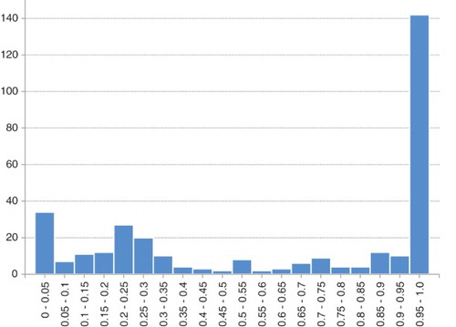
Table 5. Determinants of discretionary depreciation utilization

N = 330	Utilization	Utilization	Utilization	Utilization
	(1)	(2)	(3)	(4)
Intercept	0.65	0.51	0.65	0.69
	(8.02)***	(6.29)***	(8.30)***	(9.07)***
Lossit	−0.23		−0.25	−0.29
	(−2.06)**		(−2.29)***	(−2.66)***
NetIncit		0.00
		(1.72)*
TLCFit	−0.27	−0.27	−0.27	−0.25
	(−4.14)***	(−4.07)***	(−4.17)***	(−4.16)***
MTR52it	0.16	0.27	0.18	0.12
	(1.89)*	(3.63)***	(2.19)***	(1.54)
MTR42it	−0.05	0.09	−0.03	−0.06
	(−0.55)	(1.33)	(−0.39)	(−0.72)
MTR33.5it	−0.24	−0.08	−0.23	−0.23
	(−2.41)**	(−0.88)	(−2.38)**	(−2.46)***
PotThreshit			−0.12	−0.39
			(−2.46)**	(−7.66)***
Threshit				0.44
				(7.46)***
TAit	−0.00	−0.00	−0.00	−0.00
	(−1.08)	(−1.33)	(−0.65)	(−0.59)
Y2009t	0.08	0.07	0.06	0.04
	(1.47)	(1.42)	(1.13)	(0.74)
Y2010t	0.13	0.12	0.12	0.11
	(3.29)***	(3.11)***	(2.99)***	(2.78)***
Prod	0.01	−0.01	0.02	0.02
	(0.18)	(−0.17)	(0.23)	(0.28)
R^2	0.31	0.31	0.33	0.41

Notes: *,**,*** indicate significance at the 10%, 5%, 1% level. Between brackets we report t-values based on are based on clustered (by firm) robust standard errors (Petersen, 2009).

In this table we report the results of regression models where the dependent variable is utilization rate of discretionary depreciation. Column 1 reports results of the main model without the smoothing effect. In Column 2 we replace the loss variable with the actual profit number. Column 3 reports results of Equation (4). In Column 4, we also include the variable Thresh_itwhich is 1 for firms that due to discretionary depreciation move to a lower tax bracket.

Main regression model: (4)

Column 1 shows the results without the smoothing indicator. As predicted in H2b and consistent with Aarbu and MacKie-Mason (2003), firms with a loss carryforward have lower utilization rates, as do firms that made a loss (Loss_it = 1). Furthermore, as predicted in H2a, when the owner of a firm has a higher marginal tax rate (before depreciation), the firm has a higher utilization rate (β₃ > β₄ > β₅). A Wald test shows that these differences are statistically significant (F-value = 47.68, df_2,320, p < .01). Let us consider for example firms in the highest tax bracket. If we assume that they have no loss carryforward (and they clearly did not make a loss), we find a rate of utilization equal to 81% (0.65 + 0.16) in 2011 if we ignore the contribution of insignificant variables; in 2010 it was even higher (94%). In Column 2, we measure performance by income instead of by a loss dummy and find that firms that are more profitable have higher utilization rates. When firms make a small profit or no profit at all, it does not pay for them to depreciate large amounts. They can better save that tax deduction for the future. Larger firms have lower utilization rates, although this result is insignificant in most of the models. Utilization rates in 2009 and 2010 are higher than those in 2011, although only the difference with 2010 is significant.

In Column 3, we report our finding that firms that would end up in a lower tax bracket, for instance that would be subject to a 42% tax rate rather than a 52% one, if they depreciated maximally (PotThresh_it = 1), had a lower utilization rate. Firms file their tax form of a year during the next year and therefore already have some indication about their profit in the ongoing year. Clearly, when such firms approach a lower tax bracket threshold they have an incentive to save depreciations, as we predicted in H2c. The average utilization of these firms is 12% less. This suggests that firms used the DTD rule to smooth their taxable income, which can be very valuable in a progressive tax system (Berg et al., 2001; Wielhouwer et al., 2002). We show in a separate online Appendix that this indeed may reduce expected tax payments. Column 4 reports results when adding a dummy variable indicating whether the firm not only could but also did enter a lower tax bracket due to discretionary depreciation (Thresh_it = 1). The descriptive statistics show that in 26% of the firm-years firms would fall into a lower tax bracket if they depreciated maximally (PotThresh = 1). Yet, only 16% do fall into a lower bracket after depreciation, i.e. 10% do not. The fact that the coefficient of Thresh_it is similar to that of PotThresh_it indicates that firms that do not smooth their taxable income, that is they continue to depreciate despite the decrease in the marginal tax benefit, behave in a way that is similar to firms that would be in a given tax bracket regardless of their depreciation charge. However, firms that decide to save the right to depreciate shift on average 39% of the available depreciation charge to future years.

Why do some firms, sometimes, bank the right to depreciate in order to smooth profits, while others decide to use-up the depreciation options despite the decline in marginal value? To answer this we looked at the 85 firm-years that could have ended-up being in a lower tax bracket by fully depreciating (i.e. PotThresh_it = 1). Figure 2 shows how they are distributed over the marginal tax rate categories.

Figure 2. Distribution of smoothing vs. not smoothing over the marginal tax rate categories. Panel A: absolute frequencies. Panel B: relative frequencies

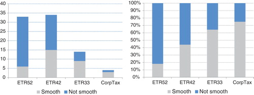
As we show in both panels of Figure 2, smoothing occurs in each category, although smoothing occurs more frequently when the marginal tax rate is lower. This may be for several reasons. First, at the lowest marginal tax rate (33.5%) smoothing does not reduce current tax payments because both when smoothing and when not smoothing the marginal tax rate will be zero. Therefore the opportunity costs of smoothing are low. More depreciation is most likely added to the loss carryforward, and the gain in another year is at least 33.5% when a profit is made. Note however that not smoothing is not necessarily irrational as there may be some carryback possibilities (on which data are not available). Second, the lower the current marginal tax rate, the higher the possible gain of a tax saving in the future. Finally, not depreciating is more risky in higher tax brackets. It is possible for a firm to be subject to a lower marginal tax rate in the future. Hence, the risk of smoothing increases with the marginal tax rate.

In order to further explore what drives smoothing we use the following regression equation: (5) in which

• Smooth_it = (1-Thresh_it) = equal to 1 if firm i in period t has the same marginal tax rate (MTR) before and after depreciation, and 0 if it has not.

• MTRvar_i = the number of changes in tax brackets over the 4 years of data for firm i.

Other variables are as defined before.

Table 6 reports the results of this regression.

Table 6. What determines whether a firm smoothes?

N = 85	Smooth
	(1)
Intercept	2.94
	(2.18)**
TLCFit	1.25
	(1.56)
WCapit	0.00
	(1.88)*
MTR52it	−3.98
	(−2.88)***
MTR42it	−2.49
	(−1.86)*
MTR33.5it	−1.70
	(−1.22)
MTRvar	−1.49
	(−2.50)**
R^2	0.22

Notes: *,**,*** indicate significance at the 10%, 5%, 1% level. Between brackets (z-values) based on Huber White standard errors are reported.

In this table we report the results of a logit regression model of Equation (5). The dependent variable is an indicator whether a firm that could smooth taxable income, actually did smooth its taxable income. (5)

We find that firms with lower levels of working capital, which may for an important part consist of cash, save depreciation less often. This is to be expected as they are more likely to be in need of cash and therefore are more likely to choose to lower their current tax payments if they can. We find too that firms that have a higher variation in marginal tax rates (MTRvar) smooth less often. A higher MTRvar indicates that the tax rate for the next year is more uncertain in which case one would expect there to be a preference for paying less tax immediately. Firms with a higher marginal tax rate are also less likely to smooth (β₃ > β₄> β₅), which is confirmed by a significant Wald test (F = 6.60, df_2,78, p < .01). To provide further descriptive evidence whether smoothers and non-smoothers made the right choice, we analyze whether next year’s tax rate of these firms was higher, equal, or lower than the current tax rate. Since for this analysis we need the tax rate for the next year, we only have 43 observations left. Only 1 firm of the 29 firms (out of these 43) that did not smooth had a higher tax rate in the next year; 16 had an equal tax rate and 12 had a lower tax rate in the next year. For the remaining 14 observations that did smooth, 2 ended up with a higher tax rate in the next year, and 5 with a lower tax rate. Overall, 6 of the 43 firms may have made with hindsight the wrong decision: 1 did not smooth and ended up in a higher bracket next year, and 5 did smooth and ended up with a lower tax rate next year.

7. Conclusion

In this paper we use a sample of relatively small, agricultural firms to investigate the utilization and eventual effects of DTD rules introduced in the Netherlands during the economic crisis of 2009–2011 to stimulate investments. Compared to the bonus depreciation possibilities introduced in the US in 2001, in the Netherlands firms were given the option to (i) depreciate more accelerated also in later years following an investment and (ii) depreciate less, that is, to postpone depreciation, which could make the rule also valuable for firms with low profits, a loss, or a loss carryforward.

Using Monte Carlo simulations, we find that in many circumstances, especially when income is uncertain or low in the near future, the discretionary depreciation options as offered by the Dutch program lead to higher expected present values of tax deductions which increases the expected net present value of investments in case of limited carryforward possibilities. Our empirical results indicate that due to this rule, investments in assets that qualify for this DTD, crowded out investments that did not qualify. Only for firms that faced the highest marginal tax rate, this effect is not found. These firms invested more due to the regulation. In that sense, the regulation was limitedly successful in stimulating investments.

Generally, the firms that invested in assets for which DTD was admitted were larger, paid a higher marginal tax rate, and less often had a loss carryforward. These results together indicate that also distributional concerns should be taken into account when offering temporary flexibility in depreciation. Although one could argue that this regulation distorts competition and unfairly benefits firms with high marginal tax rates, one could also argue that competition was already distorted due to the progressive tax system and the regulation only removes an unfair burden for these high marginal tax rate firms. Our results indicate that the additional investments of these firms due to DTD more or less offset the disincentive that these firms in general have.

Finally, our results show that firms used the flexibility of DTD to smooth their taxable income under the progressive tax system, that is, firms did not depreciate to the maximum permitted in order to save depreciation charges for the future when they may face a higher tax bracket. Firms that could end up in a lower tax bracket by depreciating maximally, on average depreciated 12% less of the available depreciable amount. Those who decided to smooth, shifted on average 39% to future years. Whether firms decided to smooth taxable income depended on their cash position, the marginal tax rate, and the risk of being subject to a lower marginal tax rate in the future.

In our study, we consider whether the regulation was effective by investigating whether firms in general, and firms with a high marginal tax rate specifically, invest more than expected based on observed and unobserved factors. Moreover, the data allow to study crowding out effects in detail which is not possible when considering total levels of investments only. The limitation is, however, that our data do not allow to study this question by means of a difference-in-difference design as these detailed data are not available over a long time period. Although this is a limitation of the study, a complete design is difficult anyway as the crisis was global so that a comparison with levels in the absence of the regulation are not available. For future research it may be interesting to compare investment levels between countries with and without these regulations that did all face an economic crisis.

Our analyses is based on a population consisting of relatively small private firms in only one sector (agriculture). For this population we had access to details about the distinction between the types of assets invested in and the actual tax depreciation rates chosen by the firms. This allows us to answer questions on crowding out in more detail and to analyze the actual use of depreciation flexibility, but it might limit the generalizability of the results. Knittel (2007) indeed points to differences between take-up rates of bonus depreciation across industries. Firms in an industry consisting of many small firms with low investment levels, such as agriculture, make less use of bonus depreciation than firms in an industry with a small number of large firms. This suggests that results in other industries may be different and that the regulation may yield stronger effects in many other industries. We believe that our results can be generalized to firms with similar characteristics (relatively small private firms, with owners that face a progressive tax rate) as the incentives are not specific to the agricultural industry.

The results of our study may inform policy makers regarding stimulating effects of flexible depreciation possibilities. One argument that has been made against the effectiveness of merely bonus depreciation is that it is of low value for firms that are not profitable or that have a loss carryforward. An important difference between the bonus depreciation approach in the US and DTD as instituted in the Netherlands is that the second approach gives firms the option of not only accelerating depreciation, but also of postponing depreciation to later years, years in which higher depreciation was also allowed. This may be even more important during economic downturns as higher income is only expected in later years. Our sample indicates that postponing was in fact used. Under the progressive tax system that applies in our study firms used this flexibility for example to smooth taxable income. Taken together, our results suggest that a more flexible set of depreciation options compared to accelerated depreciation alone is valuable to firms and could be effective in stimulating investments especially in a progressive tax system.

Acknowledgements

We thank the Noord-Holland office of WEA Accountants & Adviseurs for generously providing access to data. We thank as well Jeroen Hauwert for collecting that data. Further, we thank Anja De Waegenaere, John Robinson, Richard Sansing, Sondra Grace, and the participants of workshops at VU University Amsterdam and Tilburg University and also attendees of the EIASM 3rd Münster Workshop of Current Research on Taxation. Their comments on earlier drafts were most helpful. Finally, we thank the handling editor (Martin Jacob) and both reviewers for their constructive comments.

Supplemental Data and Research Materials

Supplemental data for this article can be accessed on the Taylor & Francis website, doi: 10.1080/09638180.2017.1286250

Notes

1 Although such tax incentives may affect asset prices (e.g. Edgerton, 2011), these benefits are unlikely to be offset completely in the short run by these implicit taxes (House & Shapiro, 2008).

2 One exception is De Waegenaere and Wielhouwer (2011), who study the optimal tax depreciation method choice when the firm may with some probability switch to another depreciation method.

3 Cf. Regeling 10 Mei. 2010 nr. DB 2010/103M, Staatscourant 2010, 7724l https://www.rijksoverheid.nl/documenten/besluiten/2010/05/19/wijziging-van-de-uivoeringsregeling-willekeurige-afschrijving-2001. At the start of the regulation, firms were allowed to depreciate 50% in the first year and only maximally 50% in the second year (cf. Regeling 10 December 2008 nr. DB 2008/697M, Staatscourant 2008, nr. 246). In May 2010, the rule was made more flexible, retroactive to 1 January 2009.

4 Using longer asset lives will increase the expected benefits from bonus and discretionary depreciation as the benchmark of straight line depreciation defers tax deductions to later periods. DTD will also become more beneficial compared to bonus depreciation as under bonus depreciation the residual tax base of the asset is divided over more years, while under DTD the firm has the option to depreciate entirely the investment in earlier years.

5 When losses can be carried forward, deductions in excess of taxable income are not necessarily lost but may be compensated in future years. This implies that differences between depreciation methods become less important. The depreciation method is however still relevant when the loss carryover period is limited (Kulp & Hartman, 2011). When loss carryforward is limited, DTD has an additional advantage: depreciation can be postponed until the loss carryover is fully used up which reduces the probability of the loss carryover expiring unused.

6 The firms that have missing values for 2011, on average invested more in 2009 and 2010, were more profitable and used the regulation more often. Analyzing our models without observations from 2011 does however lead to the same conclusions.

7 The sample is reduced from 325 to 318, because for 7 firms we do not have complete carryforward information.

8 Including indicator variables for many marginal tax rates and their interactions leads to multicollinearity issues. We therefore confine our attention to the highest marginal tax rate.

9 During the period of the study the relevant tax percentages were 33.5% (≈0–18,000 euro’s), 42% (≈18,000–55,000), or 52% (>≈55,000) for individuals. The exact thresholds differ slightly over years. The corporate tax rates are 20% (income 0–200,000 euro’s) and 25% (2011), 25.5% (2010, 2009) (income >200,000). In 2008, the cutoff value was 275,000 instead of 200,000.

10 To calculate the effective tax rate for partners of a partnership, we assume that firm profit is divided evenly between the partners.

11 In addition, the inclusion of the InvYN_it could bias the estimates for the control variables in Equation (1).

12 The DTD program started in 2009, and therefore in 2008 it is impossible to distinguish between DTD and NDTD-assets. In Equation (2), we therefore use the total investments as the values for NDTDinv_t−1 for 2008. We also replaced these values with 78% of the total investments which led to similar results. 78% is the sample average of NDTD-assets.

13 Untabulated results show that there is no industry related difference between service and trade firms. We therefore combined these two groups to increase the size of the reference group.

14 We used the Heckman two steps procedure in which the inverse Mills ratio is computed as follows. First the predicted values of the first step are computed. Then the inverse Mills ratio is computed as with z (Z) the pdf (cdf) of the standard normal distribution. We use two non-overlapping independent variables between the selection and substantive equation (i.e. the exclusion restrictions), being MTR_it−1 and Partners_it.

15 We capped the utilization rate at 100%, although the rate of some firms surpassed that. The reason that some observations have utilization rates higher than 100% is some misunderstanding concerning the reinvestment reserve in combination with discretionary depreciation. Not capping them, or excluding those observations from the analysis altogether would not change the qualitative interpretation of the results.

16 Although 11% of total assets is quite a large effect, so is the negative effect of the marginal tax rate itself. This 11% may be explained partly by some firms making very large investments relative to their assets.

17 We use an indicator variable to control for production firms vs. non-production firms. Additionally, we replaced this variable with seven indicator variables for industry: livestock; agriculture; horticulture and floriculture; other agricultural production; services; trade; other non-agricultural production. This did not affect the results.

18 Lennox, Francis, and Wang (2012) warn for the problem of high multicollinearity between the inverse Mills ratio and the main variable of interest. To mitigate this problem, in our specifications we include independent variables in the selection model that are not included in the treatment effect model (i.e. the so-called exclusion restrictions). As a result, the Variance Inflation Factor of the inverse Mills ratio is only 4 in our study.

19 Equations (1) and (2) only differ in their dependent variable and the independent variable Inv_i,t−1. Errors of both equations could be correlated especially when both equations would have the same omitted variables. Therefore we also estimated a Seemingly Unrelated Regression model. This analysis also shows that Use_it is significantly negative for Equation (2) but not significant for Equation (1). In addition, a Wald test shows that the coefficient for Use_it in eq.1 is significantly larger than the Use_it coefficient in Equation (2) (χ² = 112, p < .01).

20 The firms are advised by different auditors of the firm and it would therefore be possible that we find ‘auditor effects’ in the utilization rates. The utilization rate is however not significantly different for the 19 different auditors.

References

- Aarbu, K. O., & MacKie-Mason, J. K. (2003). Explaining underutilization of tax depreciation deductions: Empirical evidence from Norway. International Tax and Public Finance, 10, 229–257. doi: 10.1023/A:1023835513759
- Berg, M., De Waegenaere, A., & Wielhouwer, J. L. (2001). Optimal tax depreciation with uncertain future cash-flows. European Journal of Operational Research, 132, 197–209. doi: 10.1016/S0377-2217(00)00132-6
- Cohen, D., & Cummins, J. (2006). A retrospective evaluation of the effects of temporary partial expensing. Finance and Economics Discussion Series, Divisions of Research & Statistics and Monetary Affairs, Federal Reserve Board, Washington, DC.
- Cohen, D. S., Hansen, D.-P., & Hassett, K. A. (2002). The effects of temporary partial expensing on investment incentives in the United States. National Tax Journal, 55, 457–466. doi: 10.17310/ntj.2002.3.05
- De Waegenaere, A., & Wielhouwer, J. L. (2002). Optimal tax depreciation lives and charges under regulatory constraints. OR Spectrum, 24, 151–177. doi: 10.1007/s00291-002-0096-0
- De Waegenaere, A., & Wielhouwer, J. L. (2011). Dynamic tax depreciation strategies. OR Spectrum, 33, 419–444. doi: 10.1007/s00291-010-0214-3
- Edgerton, J. (2010). Investment incentives and corporate tax asymmetries. Journal of Public Economics, 94, 936–952. doi: 10.1016/j.jpubeco.2010.08.010
- Edgerton, J. (2011). The effects of taxation on business investment: New evidence from used equipment (Working Paper). Federal Reserve Board.
- Edgerton, J. (2012). Investment, accounting, and the salience of the corporate income tax (No. w18472). National Bureau of Economic Research.
- Eichfelder, S., & Schneider, K. (2014). Tax incentives and business investment: Evidence from German bonus depreciation (CESifo Working Paper No. 4805). Center for economic studies & Ifo Institute.
- Hall, R. E., & Jorgenson, D. W. (1967). Tax policy and investment decisions. American Economic Review, 57, 391–414.
- Hanlon, M., & Heitzman, S. (2010). A review of tax research. Journal of Accounting and Economics, 50, 127–178. doi: 10.1016/j.jacceco.2010.09.002
- Heckman, J. J. (1976). The common structure of statistical models of truncation, sample selection, and limited dependent variables. Annual Economic Social Measures, 5, 475–492.
- House, C. L., & Shapiro, M. D. (2008). Temporary investment tax incentives: Theory with evidence from bonus depreciation. American Economic Review, 98, 737–768. doi: 10.1257/aer.98.3.737
- Hulse, D. S., & Livingstone, J. R. (2010). Incentive effects of bonus depreciation. Journal of Accounting and Public Policy, 29, 578–603. doi: 10.1016/j.jaccpubpol.2010.06.008
- Huston, G. R. (2010). The implications of increased depreciation allowances on firms’ capital expenditures and leasing transactions (Working Paper). Florida State University.
- Jackson, S. B., Lui, X., & Cecchini, M. (2009). Economic consequences of firms’ depreciation method choice: Evidence from capital investments. Journal of Accounting and Economics, 48, 54–68. doi: 10.1016/j.jacceco.2009.06.001
- Klemm, A. (2010). Causes, benefits, and risks of business tax incentives. International Tax and Public Finance, 17, 315–336. doi: 10.1007/s10797-010-9135-y
- Knittel, M. (2007). Corporate response to accelerated tax depreciation: Bonus depreciation for tax years 2002–2004 (OTA Working paper series).
- Kosi, U., & Valentincic, A. (2013). Write-offs and profitability in private firms: Disentangling the impact of tax-minimisation incentives. European Accounting Review, 22, 117–150. doi: 10.1080/09638180.2012.661938
- Kulp, A., & Hartman, J. C. (2011). Optimal tax depreciation with loss carry-forward and backward options. European Journal of Operational Research, 208, 161–169. doi: 10.1016/j.ejor.2010.06.040
- Lennox, C. S., Francis, J. R., & Wang, Z. (2012). Selection models in accounting research. The Accounting Review, 87, 589–616. doi: 10.2308/accr-10195
- Petersen, M. A. (2009). Estimating standard errors in finance panel data sets: Comparing approaches. Review of Financial Studies, 22, 435–480. doi: 10.1093/rfs/hhn053
- Porcano, T. M. (1984). The perceived effects of tax policy on corporate investment intentions. Journal of the American Taxation Association, 6, 7–19.
- Porcano, T. M. (1987). Government tax incentives and fixed asset acquisitions: A comparative study of four industrial countries. Journal of the American Taxation Association, 9, 7–23.
- Poterba, J., Rao, N., & Seidman, J. (2011). Deferred tax positions and incentives for corporate behavior around corporate tax changes. National Tax Journal, 64, 27–57. doi: 10.17310/ntj.2011.1.02
- Richardson, S. (2006). Over-investment of free cash flow. Review of Accounting Studies, 11, 159–189. doi: 10.1007/s11142-006-9012-1
- Rose, C. C., & O’Neil, C. J. (1985). The viewed importance of investment tax incentives by Virginia decision makers. Journal of the American Taxation Association, 7(1), 34–43.
- Shackelford, D. A., Slemrod, J. & Sallee, J. M. (2011). Financial reporting, tax, and real decisions: Toward a unifying framework. International Tax and Public Finance, 18, 461–494. doi: 10.1007/s10797-011-9176-x
- Shin, H., & Kim, Y. H. (2002). Agency costs and efficiency of business capital investment: Evidence from quarterly capital expenditures. Journal of Corporate Finance, 8, 139–158. doi: 10.1016/S0929-1199(01)00033-5
- Wakeman, L. M. (1980). Optimal tax depreciation. Journal of Accounting and Economics, 2, 213–237. doi: 10.1016/0165-4101(80)90003-8
- Wielhouwer, J. L., De Waegenaere, A., & Kort, P. M. (2002). Optimal tax depreciation under a progressive tax system. Journal of Economic Dynamics and Control, 27, 243–269. doi: 10.1016/S0165-1889(01)00034-3