Bent Hansen’s theory of inflation 1951¹

Abstract

Bent Hansen’s analysis of repressed and open inflation was to some extent based on microeconomics, he analysed the interaction between wage and price inflation and discussed economic policy problems when there were goals in addition to that of curbing inflation. Hansen was influenced by Erik Lindahl who, like the other members of the Stockholm School was critical to the quantity theory of money. Hansen’s book contains early analyses of spill-over effects and building blocks of the supply multiplier.

Keywords:

• Inflation
• Stockholm School
• quantity theory

JEL CODES:

• B22
• B25
• E31

The Keynesian  theory had its root in the persistent unemployment of the 1930s whereas excess demand and repressed or open inflation dominated during the years after WWII. However, despite advances in monetary analysis during the 1950s and 60’s it was not until around 1970 that the income-expenditure model was seriously challenged. The discussions of Phelps (1967) and Friedman (1968) about the possible existence of a natural (or equilibrium) rate of unemployment can be seen as a symbol of the new orientation of macroeconomic research. Here the long run rate of unemployment was not a function of aggregate demand (variations in demand would instead lead to movements along the short-run Phillips curve) but depended instead on frictions and structural imbalances in the economy.

In spite of this general picture there was much research done during the 1940s, 50 s and 60 s of the mechanisms behind inflation, with Keynes (1940) as one of the contributions. Bent Hansen’s analysis of repressed and open inflation is a good example of this research.² It was to some extent based on microeconomics, analysed the interaction between wage and price inflation and discussed economic policy problems when there were goals in addition to that of curbing inflation. Hansen was influenced by Erik Lindahl who, like the other members of the Stockholm School,³ was quite critical to the quantity theory of money.

I first give a back-ground to Hansen’s work and an overview of the analysis and results of his dissertation A Study in the Theory of Inflation. After that follows a section on the public defense of his thesis with special reference to the problem of disequilibrium dynamics. In the rest of the paper the following items are treated: spill-over and multiplier effects, the quantity theory of money and finally expectations and the real rate of interest. A summary concludes the paper.

The back-ground

The world-wide inflation of the Korea crises had not yet occurred when Hansen began his work in 1948. The subject of the dissertation was nevertheless of current interest because of the extensive inflation during and after WWII, see Brown (1955). It is true that Keynesianism was advancing strongly in the end of the 1940s. Here national income and employment were pointed out as important endogenous variables. The price level was not in the same way central to the analysis. Keynes himself had on the other hand already in 1940 in How to Pay for the War analysed situations with overfull employment.

Inflation could be analysed from several starting-points. One was the quantity theory of money which Hansen p. 1 repudiated with the argument that inflation then was identified by an increased volume of money. A flagrant example according to Hansen referring to Bresciani-Turroni (1937, 155 et seq.) of when this method went wrong was during the German hyper-inflation in 1923 when price level increases continued in spite of a constant quantity of money.⁴

Bent Hansen’s critical attitude to the quantity theory was probably a result of the environment in which he worked. The Swedish economists of the time were critical to the theory. Hansen’s tutor, Erik Lindahl (1929a), had published a paper in which he discussed the shortcomings of the quantity theory. Another example is Ohlin (1943) which contains a comparison between the Stockholm School approach and the quantity theory.

The critical attitude to the quantity theory can be traced back to Knut Wicksell’s monetary analysis. Wicksell’s (1898) work in monetary theory implied the development of an alternative to the quantity theory of money.⁵ Wicksell’s main interest was to explain price level fluctuations during the 1800s. He thereby took the development of the banking system and its capacity to mediate payments into account. Since the quantity of bank money was endogenous he based his explanation on the relationship between the loan rate of interest and the rate of profit. He called the latter the natural rate of interest.⁶ One argument against the quantity theory was consequently that it assumed an exogenous quantity of money and this assumption did not fit very well with the development of the modern payments system.

An alternative to the quantity theory of money was to start from the Keynesian inflation analysis in How to Pay for the War. But Bent Hansen p. 250 did not think that this was a reasonable starting point since Keynes only studied the excess demand in an aggregate goods market: “Keynes’ General Theory has, unfortunately, given rise to a habit of thought in inflation theory according to which ‘demand for commodities is also demand for labor’. We have tried to remove this bad habit of thinking from our models.” The labour market is consequently according to Hansen not a simple reflection of the goods market.

Hansen’s starting-point was instead the Swedish tradition from Knut Wicksell. In his lectures from 1906 Wicksell had stressed that increases of the general price level have the same causes as an increased price in an individual market. The price change is in both cases caused by an excess demand. Hansen’s p. 2 comment was that “the foundation was laid for an integration of the micro and macro-theory in this field”. Wicksell had also analysed the interaction between the price and wage movements during an inflation process in the central section of chapter 9B in Geldzins und Güterpreise from 1898.⁷ However, in contrast to Wicksell’s theory of the inflation process Hansen did not integrate the development of the money markets in his analysis.

Price changes according to the quantity theory of money imply comparative statics. This is in contrast to Wicksell’s cumulative process.⁸ It is true that Wicksell in his chapter 9B assumed a successive equilibration in the beginning of each period of first the labour and then of the goods market, but it did not lead to a simultaneous equilibration of the markets. The result was cumulative wage and price increases that did not eliminate the gap between the natural and the loan rate of interest. Bent Hansen’s insistence that both the aggregate goods and the labour market should be included in the analysis therefore gives a direct link to Wicksell’s cumulative process.

Bent Hansen analysed a topical problem of the late 1940-ies when he choose to study the inflation problem. He furthermore build on a long Swedish tradition. There was however a third aspect of his dissertation, the choice of method. Hansen’s investigation was built on a solid mathematical ground and his method of attacking his problem i strikingly modern. Both Knut Wicksell and Erik Lindahl used mathematics with great skill so Hansen had good precursors to follow. In addition John R. Hicks’ (1939, 1946) influential book Value and Capital contained a mathematical introduction to general equilibrium analysis and a first (static) attempt to tackle the related stability problem. Paul Samuelson’s (1947) Foundations of Economic Analysis may to begin with not have had as wide an impact as Hicks’ book, but it demonstrated the power of translating ordinary language into mathematics and in this way guarantee that the conclusions followed logically from the assumptions. Hansen (1951) referred both to Hicks (1946) and to Samuelson (1947) but the influence of the latter seems to be greater.

Despite the influence of Samuelson's Foundations which relied on analytical methods, Hansen presented his analysis to a considerable extent with diagrams. The reason was probably pedagogical, the average economist in 1951 was not supposed to master algebraic presentations and even less to understand how to solve systems of differential equations.⁹ The heavy mathematics was therefore concentrated to chapter VIII and its appendix where Hansen analysed an economy with n + 1 markets. Diagrams are however problematic when it comes to illustrate multidimensional problems such as these that appear when more than one market should be illustrated. Hansen’s solution was to present the aggregate goods market in the diagrams and to indicate how the supply side would be affected by excess demand in the aggregate labour market.

Temporary equilibrium, ex ante gaps and inflationary gaps

In temporary equilibrium the plans of the individual firms and households are coordinated during the individual period. Price changes only occur in the joint between periods. The economic agents are planning for many periods ahead but revise their plans when they receive new information in the beginning of each period. The theory of temporary and intertemporal equilibrium respectively was developed by Lindahl (1929b).¹⁰ The theory of temporary equilibrium, often attributed to Hicks was first developed by Lindahl (for a discussion, see Siven 2002).

During the 1930s the period analysis was further developed by the Stockholm School. The assumption of temporary equilibrium was often dropped and various types of disequilibrium situations were studied.¹¹

In chapter II Hansen’s discussion starts from the period analysis of the Stockholm School where each period is assumed to be so short that no price changes take place during the individual period.¹² The difference between planned purchases and expected sales in a market (monetary excess demand, i. e. quantitative excess demand multiplied by the market price) in the beginning of the period (ex ante) is registered at the end of the period (ex post)¹³ and can together with information about the course of events during earlier periods form the starting point for pricing and other planning for the next period.¹⁴

Period analysis was usually applied to situations where the plans of the different households and firms were not mutually consistent (the sum of the planned purchases of a certain commodity could differ from the sum of the expected sales of the firms) but the plans of the individual economic subjects were internally consistent. In the present case this means that they in their planning inter alia take their budget equations into consideration. These equations are according to the assumptions of the period analysis based on constant prices during the period.

If the budget equations hold and all households and firms are confronted by the same prices during the period then the sum of the monetary excess demands over all the markets of the economy will be equal to zero. For a model with one commodity and one factors market¹⁵ this means that the monetary excess demands of these two markets equals the sum of the monetary excess supplies of the claim markets and the money market.

An economy without government or international trade is analysed on pp. 36–37. Here the incomes of entrepreneurs and of workers are defined as well as saving. Hansen then shows that the difference between the investments and saving ex ante equals the sum of the ex ante commodity gap (planned purchases of commodities minus expected sales of commodities) and the ex ante factor gap (planned purchases of factors minus expected sales of factors), see equation II:5 on p. 37. Hansen called this equation the fundamental equation of the Stockholm School.¹⁶

A monetary pressure of inflation is by definition at hand if at least one of the ex ante commodity gap or the ex ante factor gap is positive and no one of the two gaps is negative. According to the fundamental equation of the Stockholm School this means that the difference between investments and saving is positive if there is a monetary pressure of inflation, but the reverse does not hold.

The discussion above is based on the period analysis of the Stockholm School and contains no behavioural assumptions except that the individual budget equations hold. In chapter III Hansen takes a first step towards analysing the actual circumstances during an inflation. The concept of inflationary gap is introduced. The difference between this concept and the ex ante gap is connected to the interpretation of demand and supply, respectively.

For demand Hansen introduced two demand concepts in addition to planned purchases, namely optimal purchases and active attempts to purchase. Optimum purchases are “those purchases which it would be worth-while to make from the point of view of a ‘rational’ calculation (of utility or costs) if the economic subject where free in this respect, within his financial resources and within that framework of legal restrictions which is assumed to be given (optimum purchases must exceed or equal planned purchases)” (p. 24). Active attempts to purchase are “the purchases which the economic subject tries to carry out by making binding offers of purchase (giving orders); the active attempts to purchase will never be less than the planned purchases, and they can be greater than the optimum purchases.” (p. 24). The signal system of the market may consequently be distorted by the excess demand since buyers may offer to purchase larger quantities than they actually need, in order to secure more of the scarce supply.

As to the supply side the expected sales is not a good measure of supply since production possibilities are in focus during inflation. The production possibilities of the firms may be restricted by the availability of labour force. This means that an excess demand in the labour market can have a direct quantitative effect on supply in the commodity market. The firms may therefore be subject to a rationing restriction in the labour market so that their effective supply function is substituted for their notional supply function.¹⁷

The supply of labour may likewise be affected by households being subject to rationing in the commodity market. It is no longer the notional supply which describes labour supply but the effective supply function. The latter function is in contrast to notional supply not only a function of prices but of rationing restrictions as well. Utility maximisation is in the latter case not only subject to the budget equation but also to one or several rationing restrictions.

In order to stress the above mentioned aspects Hansen introduced a new concept, inflationary gaps. Monetary excess demand is the basis for both ex ante gaps and inflationary gaps, but the interpretation of the demand and supply concepts are different for ex ante gaps and inflationary gaps.

Two different questions are of interest during demand inflation, how much must excess demand be decreased in order to attain equilibrium and what price increase will be generated by the excess demand?

For the first question the inflationary gap in the commodity markets is defined as optimum purchases of commodities - value of the available quantity of commodities. The inflationary gap in the factor market is analogously defined.

The second question instead gives the definition that the inflationary gap in the commodity markets is defined as active attempts to purchase - value of the available quantity of commodities. The inflationary gap in the factor market is analogously defined.

The demand and supply concepts are changed when we talk about inflationary gaps instead of ex ante gaps. The definition of a monetary pressure of inflation then changes so that a monetary pressure of inflation is at hand if there is an inflationary gap in the commodity and/or the factor market and neither of the two gaps is negative.

The result derived in chapter II that the difference between the investments and saving ex ante equals the sum of the ex ante commodity gap and the ex ante factor gap does not hold when we substitute the inflationary gap for the ex ante gap in the commodity market and in the factor market, respectively. The reason is that the demand and supply concepts that are involved in the definition of the ex ante gap are different from those in the inflationary gap, see Hansen’s discussion on pp. 72 − 78.

After discussing the three different aspects of demand, planned demand, optimum demand and active attempts to purchase, Hansen choose to abstract from the differences between the three concepts. However, he kept using the available quantity on the supply side, thereby taking rationing effects into consideration. If nothing else is said we in the following by “gap” will mean “inflationary gap” so that the effective supply function, not the notional one, is involved in the monetary excess demand.

Repressed inflation

During and after WWII both belligerent and non-belligerent countries had applied regulations of different kinds. One of the goals was to hinder excess demand in the goods and factor markets to result in price increases. In addition to direct interventions in the production process and in the distribution of the result of production, price- and wage-regulations were important instruments, see Lundberg (1953, chapter 15), Brown (1955, chapter 7) and Lindbeck (1975, chapter 2). Hansen therefore analysed both open and repressed inflation. In the latter case price- and wage regulations means that excess demand of goods and services does not affect the general price level but instead results in rationing.

Hansen’s analysis of repressed inflation is based on a model with one aggregate commodity market and one aggregate labour market. There is no international trade and no payments to and by the public sector. There is however government intervention in the form of price and wage regulation, “the state inters into certain considerations as deus ex machima” (p. 84). Hansen assumes that investment is controlled by the state.¹⁸ Two market forms are analysed, perfect competition and monopoly but only the perfect competition case will be commented on.¹⁹

In repressed inflation the price is set below the equilibrium price by the price-control authority. If in addition the wage-rate is also controlled the marginal cost curve will lie under the corresponding curve if the labour market was in equilibrium at a higher wage level. However, the labour market is not in equilibrium and this means that the firms cannot freely vary their production. The slope of the marginal cost curve is vertical at the point where the firms cannot get hold of more labour.

When analysing repressed inflation in chapter IV, Hansen used diagram 1 on p. 87 to illustrate the development in the aggregate goods market. The notional quantitative supply of commodities is under perfect competition given by the aggregated marginal cost curve (the individual marginal cost curves are summed horizontally). It is assumed that the effective supply of commodities may be smaller than the notional supply due to rationing in the labour market. This is reflected by the (effective) marginal cost curve being vertical at the quantity $Q_1$ where the firms cannot get hold of more labour, see Figure 1. This volume of production is via the aggregate production function given by the supply of labour, which is rationed due to excess demand in the labour market. The variable costs consist only of wages.²⁰

Figure 1. The aggregate perfect competitive goods market under repressed inflation. The price level is set to p₀. The supply curve consists of the aggregate marginal cost curve m. c. up to the quantity Q₁, which is the maximum possible goods production given the available quantity of labour. After that follows a vertical part B₁B₂. The quantitative excess demand in the commodity market equals D₁ - B₁, the ex ante commodity gap equals the area B₁Q₁D₀D₁ and the inflationary gap in the labour market the area B₂Q₁D₀D₁. Excess demand in the aggregate factor market is reflected in how much more goods the firms would like to produce if there was no rationing in the labour market, Q₀ - Q₁. The inflationary gap in the labour market equals the area B₂Q₁Q₀C₁ and unexpected income loss by the firms area B₁B₂C₁. The income loss is equal to the expected profit on production which could not be realised due to shortage of labour.

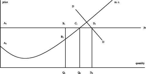
The expected sales curve is under perfect completion given by the price line. The price line reflects price control and lies below the potential equilibrium price line.²¹ The incomes of workers are given by the area under the marginal cost curve up to the volume of production $Q_1.$ Entrepreneurial incomes are likewise given by the area between the price line and the marginal cost curve up to $Q_1.$ The inflationary gap in the commodity market is a monetary excess demand and therefore indicated by an area in the figure.

The market quantitative demand for commodities is a function of the price and implicitly on total incomes and the distribution of incomes between workers and entrepreneurs which in turn depend on the wage rate. Analogous to Lindahl (1939) Hansen assumed that the marginal propensity to consume is greater for workers than for entrepreneurs. The assumption indicates a negative slope of the demand function for commodities as indicated in Figure 1.²²

The aggregate commodity market is discussed in some detail via diagrams. The conclusion is that the regulated price level (lower than the price level that would give equilibrium in the commodity market) in combination with the excess demand in the labour results in a lower quantity of production. The analysis of the commodity market was not combined by Hansen with a corresponding analysis of the labour market. Hansen however assumed that wage control results in excess demand in the labour market. The excess demand in the labour market is accentuated by the excess demand in the goods market leading to rationing of consumption and thereby to a lower supply of labour. The rationing of consumption means that the notional supply function of labour is substituted for by the effective supply function of labour.

Stabilisation policy under repressed inflation

Policy prescriptions are more complex in Bent Hansen’s analysis that in the Keynesian one. The reason is that in contrast to the Keynesian case the labour market is included in Hansen’s analysis. One example is that repressed inflation cannot be eliminated by higher taxes since it may only eliminate the inflationary gap in the commodity market whereas the inflationary gap in the labour market gap remains unaffected. The inflationary gap in the labour market will increase if prices are allowed to increase while the wage-level is fixed. The effect on the commodity-gap depends on the slope of the demand curve for commodities.

The reason for the difficulty to simultaneously eliminate the inflationary gap in the commodity and in the labour market is that more than one mean is required. The demand for commodities has to be affected in addition to letting the wage level adjust freely. An alternative is to vary government demand for labour while the price level is free to adjust. The choice of policy mix will naturally affect the real wage rate. This means that different shapings of the anti-inflation policy will have different consequences for the income distribution.²³

Open inflation

Hansen saw repressed inflation as a special case of open inflation. Prices and wages are fixed under repressed inflation either absolutely or through a highest price which is lower than the equilibrium price. Expectations are generated via a simple mechanism since one may assume that expectations are then geared to unchanged wages and prices. Prices will change under open inflation but it is still possible that the rationing mechanisms of repressed inflation may be working. This will be the case if price and wage increases are not fast enough to eliminate excess demand in the goods and factor markets. Open inflation is then studied as a non-tâtonnement process, i. e. that transactions are made before the potential equilibrium is reached, see Negishi (1962).

Hansen used two period concepts in his analysis. In chapters II to VI the length of the unit period was positive, but in chapters VII and VIII on open inflation where time derivatives were formulated the length of the period was assumed to tend to zero.²⁴ In the first set of chapters the monetary [value of] excess demand is moreover used whereas in the second set of chapters the quantitative excess demand is used. The monetary excess demand equals the price multiplied by the quantitative excess demand. The quantitative excess demand will in diagrams with quantity on the horizontal axis and price on the vertical one be depicted as the length of a line whereas the monetary excess demand will be seen as an area.

In chapter VII the assumptions of frozen prices and wages are dropped and open inflation is studied, still starting from a simple model with perfect competition, an aggregate goods and an aggregate labour market. Transactions are made outside equilibrium (non-tâtonnement). The distinction between attempted, planned and optimum demand is disregarded; demand should in principle be interpreted as active attempts to purchase, but the exact implications of this were not studied.

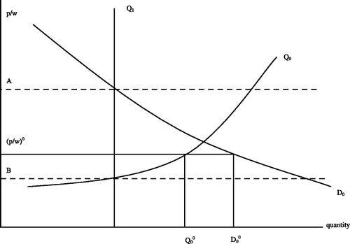
Hansen assumed that both the planned supply of goods Q₀ (which via the production function is related to the demand for labour) and the demand for goods D₀ were functions of p/w (the inverse of the real wage rate), but not of the price level. The supply of labour and consequently the actual production was assumed to be unaffected by p/w. The slope of the planned supply of commodities was positive and that of the demand for commodities was negative. The intersection of the two curves was assumed to be to the right of the actual production Q₁ so there was excess demand both in the goods and in the labour market.²⁵ The actual production, Q₁, represents the effective supply of commodities which via the production function is given by the effective supply of labour. Hansen further assumed that both the demand for labour and the demand for goods were greater than the respective supply. The price level is expected to be constant. Inflationary expectations consequently play no role in generating excess demand and thereby inflation.

There is now an inflationary gap both in the commodity and in the labour market. The rate of price increase depends on the inflationary gap in the commodity market and the rate of wage increase on the inflationary gap in the labour market.²⁶ The development of p/w consequently depends on two differential equations:²⁷ (1a) $$dp/dt=f(D_0-Q_1)$$(1a) (1b) $$dw/dt=F(Q_0-Q_1)$$(1b)

The percentage price and wage increase are equal in the stationary solution for p/w. Hansen p. 165 defined it as a quasi equilibrium since prices and wages are continuously increasing due to the excess demand for both goods and for labour. Setting $(dp/dt)/p=(dw/dt)/w$ the quasi equilibrium value of p/w is given by (2) $${(p/w)}^0=\frac{f(D_0-Q_1)}{F(Q_0-Q_1)}$$(2)

The quasi equilibrium p/w (or its inverse the real wage rate) evidently depends on how price and wage increases respectively depend on excess demand in the respective market. This means that the quasi equilibrium p/w may differ from its respective value when all markets are equilibrated. In quasi equilibrium p/w depends on the dynamic properties of the system. The capacity of the price system to collect the dispersed and fragmented information of individual economic subjects as discussed by Hayek (1945) is consequently weakened.

The distributive effect of disequilibrium can be illustrated by the thought experiment that wages are assumed to be index regulated and that the adjustment happens at regular intervals, for example once in a quarter of a year (see also the discussion on induced and spontaneous changes of prices, pp. 14–18). This means that p/w falls at regular intervals but that the system up to the next index adjustment strives to reach the quasi equilibrium. p/w will then be lower (and the real wage rate will be higher) on average than if wages were not index regulated. The quasi equilibrium can thus be manipulated and this manipulation may result in relative prices that are closer to or further removed from their equilibrium values.²⁸

Not only prices and thus the terms of the transactions are disturbed under disequilibrium. The possibilities to carry through transactions (irrespectively of the terms) are influenced. Individual firms and households are therefore affected by the exact road which the economy takes outside equilibrium. The real capital of the firms may for example be affected: “If we were further to allow for the embodiment of production decisions in some durable concrete objects, the path of the system will at any time be strewn with the remnants of past mistakes.” (Hahn 1970, 3).

Stabilisation policy under open inflation

Inflation can be eliminated if we start in a quasi equilibrium and via fiscal policy decrease the aggregate demand for goods so that the goods gap is eliminated, see Figure 2. In contrast to the case of repressed inflation it is consequently possible to close both the goods and the factor gap by only one mean, by increasing direct taxes. However, one then has to accept the effect on the real wage rate. Otherwise two means are again required, one that affects the D₀-curve, and one that affects the Q₀-curve.²⁹

Figure 2. The aggregate goods market under open inflation. Q₁ denotes production given the available labour supply, Q₀ planned supply of goods, D₀ demand for goods, A the level of p/w where the goods market is in equilibrium, B the level of p/w where the labour market is in equilibrium. (p/w)⁰ denotes the quasi-equilibrium value of p/w; here price and wage inflation are equal. In quasi equilibrium the excess demand in the goods market is given by D₀° – Q₁ and the excess demand in the labour market is implicitly given by the distance Q₀° – Q₁ (to measure excess demand in the labour market the distance measured in goods volume has to be transformed to volume of labour via the inverse of the production function).

Stability and general quasi equilibrium

The analysis of open inflation is generalised in chapter VIII in the form of a general interdependent model with n commodities, factor-services, claims et cetera. In addition there is money which also serves as the numeraire.

An appendix to chapter VIII contains a stability analysis first à la Hicks and then à la Samuelson. When applying Hicks’ method Hansen started from the assumption that all relative prices but one were at their equilibrium levels. Stability then required that an increase of the last relative price would cause excess supply in the corresponding market. On p. 210 it is pointed out that “Hicks’s conditions of stability cannot be taken as a general expression for true dynamic stability.” The problem was that Hicks did not specify a dynamic adjustment process. Hansen therefore turned to Samuelson’s method and studied the convergence of all relative prices in a system of differential equations where the rate of change of each relative price is a function of the (effective) excess demand in the respective market. Hansen studied the local stability of the system, the starting-point was assumed to be in a small neighbourhood of the equilibrium. Hansen then discussed how one could use the results of the stability analysis to draw conclusions regarding the comparative statics (Samuelson’s correspondence principle).

The rather low mathematical knowledge of the economist at the time is probably the reason why Hansen (except for a number of integrals in the chapters on repressed inflation) deported the mathematical analysis to an appendix (and illustrated the reasoning with a number of instructive diagrams). Some of the older Swedish economists were (without necessarily being unskilled in mathematics) moreover rather critical to formal analysis. One example is Lundberg (1953, 337n) who characterised Hansen work as “pure theory on an alpine level”. Hansen was however a skilled mathematician who had read and absorbed Samuelson’s Foundations. In this way Hansen was to play an important role for Swedish economic science by mediating the mathematical language which was to dominate economic analysis in the post-war period.

Determining the stationary price level

Hansen stressed (p. 162) that the model in chapter VII is inconsistent and over-determined since no price and wage level closes the model. There are three suggestions (p. 171) for making the model consistent. One suggestion is the Pigou effect,³⁰ so that demand for goods is a function of real balances, another to à la Keynes assume that lower real balances increase the rate of interest and thereby diminish the demand for goods.³¹ Investments are assumed to depend negatively on the (nominal) rate of interest. A third suggestion is that the demand for goods by the public sector is fixed in nominal terms.³² The demand for goods will then diminish when the price level increases. The above effects might according to Hansen pp. 171–172 be counteracted by depleted stocks of goods and accumulation of order stocks.

Another possibility is “to assume that the absolute price of one of the goods enters into at least one of the equations for demand or supply, for example, to assume that the supply of labour-services is a function of the money wage. But it is not possible to solve what is purely a problem of homogeneity by assuming inhomogeneity.” (p. 198). In spite of this Hansen on p. 199 discussed an equation system where the n first excess demand equations are homogenous of degree zero whereas the n + 1-th equation (excess demand for money) is homogenous of degree one in absolute prices. Hansen motivated this by referring to Walras’ law but it seems rather a way of presenting the (invalid) classical dichotomy, see Patinkin (1965, 624–629).

Walras’ law and the link to financial markets

The quasi equilibrium system is a pure real system where relative prices are determined. For the aggregate case with one goods and one factor market the real wage rate is determined. However, the goods and the factor markets are linked to the financial markets since each purchase in the goods and in the factor markets results either in a direct or in a deferred payment of equal value. The result is Walras’ law for a general equilibrium system. If all markets but one are in equilibrium then the last market will be in equilibrium as well.

Hansen’s definition of Walras’ law can be found on pp. 4–5: “The [monetary] value of excess demand for commodities and factors and claims is equal to the value of the excess supply of money. Or, as the identity can also be written, the value of excess demand for commodities, factors, claims and money is zero.” It is not stated directly that this is Walras’ law but in the index there is a reference to p. 4 under Walras’s law³³. It is also stated on p. 193 where it is formulated as “excess supply of money = value of the excess demand for all goods other than money.” Hansen’s formulation of Walras’ law is in essence the same as that of Lange (1970 [1942], 150): “Total [monetary value of] demand and total [monetary value of] supply are identically equal. […] It should be noted that Walras’s law does not require that the demand and supply of each commodity, or any of them, be in equilibrium.” Hansen referred directly to Lange (1970 [1942]) on p. 191 where Walras’ system is discussed: “That one of the equations may be derived from the others depends on what Lange has called Walras’s law.” Lange’s seminal paper is referred to on p.190.

Walras’ law builds on the consistency of the budget equations and can according to Hansen pp. 192–197 under certain conditions be generalised to hold even out of equilibrium. The requirement is that the cash budgets of the agents are consistent. The consistency requirement means for example that planned purchases may not be replaced in the analysis by active attempts to buy if these are not binding.

The value of excess demand (the ex ante gap) is defined by Hansen as the money values of planned purchases minus expected sales.³⁴ Starting from Lindahl’s (1939, 79 and 113) cash equations³⁵ Walras’ law can then be formulated in the following way: The sum of the money values of the excess demands in all markets (the money market included) equals zero. The excess demand is then defined as the difference between planned purchases and expected sales where the magnitudes are taken as they enter in the individual cash budgets. Walras’ law then does not require general equilibrium but it does require that the individual magnitudes are consistent in respect to the cash budgets (see also Barro and Grossman 1976, 58).³⁶

Walras’ law implies a connection between the goods, factor and security markets on one hand and the money market on the other. This means that the financial markets in the form of the money “market” and the security markets are formally included in Hansen’s analysis. But there is no discussion of the banking system or of individual security markets and no discussion of interest rates or security prices. Financial markets exist, at least via Walras’ law, but they are not analysed by Hansen.

Monetary equilibrium

The last chapter of Hansen’s treatise bears the title “Monetary Equilibrium”. Wicksell had according to Lindahl (1939, 246) discussed three conditions for macroeconomic equilibrium: The normal loan rate of interest should correspond to the natural rate of interest, the normal rate of interest is characterised by equilibrium between the supply and demand for saving (S = I) and the normal rate of interest implies a constant price level.³⁷ Lindahl’s discussion initiated a long discussion by Myrdal,³⁸ Ohlin and Palander, see Siven (2006). This discussion constituted one of the important themes of the Stockholm School.

Hansen’s (pp. 220 − 221) definition of monetary equilibrium was that “the sum of the values of the excess demand in all the commodity-markets is zero, and the sum of the value of the excess demand in all the factor-markets is zero.” This is in contrast to Myrdal who had defined the second condition for monetary equilibrium as equality between investment and saving ex ante. Hansen pp. 237 − 238 thought in consequence with his critique of Keynes (1940) who only took the aggregate commodity market into explicit consideration that it implies an unwarranted aggregation: “the conditions that the monetary excess demand in the composite commodity-market and the composite factor-market are each zero, imply the condition, ex ante investment = ex ante saving, assuming […] that we can identify demand with planned purchases and supply with expected sales; this assumption should usually be justified when both the inflationary gap in the commodity-markets and the factor-gap are zero. On the other hand the reverse implication is not valid. […] Myrdal’s monetary equilibrium corresponds only to the constancy of a combined commodity and factor price-index, which constitutes one of the deficiencies of Myrdal’s concept of monetary equilibrium.”

The last chapter of Hansen’s treatise also contains an analysis of how fiscal policy can be used to preserve monetary equilibrium in the event of productivity changes. The matter had been subject to a protracted discussion between Davidson and Wicksell, see Siven (1998). The question concerns whether monetary policy in the event of increased productivity should aim at a decreased price level (Davidson) or a constant price level (Wicksell). The matter was analysed by Hansen on pp. 240 − 246 where he argued that fiscal policy was a more powerful instrument then monetary policy to preserve monetary equilibrium. The reason is that fiscal policy contains several policy parameters. In Hansen’s example with decreased productivity (decreased marginal and average productivity of labour) both direct and indirect taxes can be used to affect the two gaps (the commodity-gap and the factor-gap). Hansen then shows that a combination of a decreased indirect tax and an increased income tax will imply a constant price level and preserve full employment.

Hansen’s analysis of fiscal policy in the event of productivity changes contains preliminary discussions of problems more thoroughly analysed in The Economic Theory of Fiscal Policy four years later. Here he analysed how fiscal and (to some extent) monetary policy could be used to preserve full employment and a constant price level. The last chapter of Hansen’s dissertation consequently both contains references to a long Swedish macroeconomic tradition at the same time as it points forwards to important future works.

Trygve Haavelmo’s discussion of Hansen’s analysis

Bent Hansen defended his dissertation at the University of Uppsala in May 25th, 1951. A few days later Professor Erik Lindahl wrote a pronouncement on the dissertation and the defense by Hansen dated May 29th, 1951.³⁹ Lindahl emphasised the high quality of the dissertation and stressed that the concept of quasi equilibrium was of high interest. However there had been some criticism of Hansen’s treatment of the investment-saving relationship. Moreover, the dissertation did not treat how capital accumulation was involved in the inflation process, neither the role of money. Trygve Haavelmo was first examiner⁴⁰ of Hansen’s thesis and his discussion was published i Ekonomisk Tidskrift.

Haavelmo’s main argument was that the concepts used by Hansen (for example excess demand) were not precise enough. Haavelmo (1951, 166) thought that “calculations [of differences between demand and supply] in order to get concrete contents need an addition that is not at all self-evident (but by Bent Hansen and many others is considered as self-evident), namely that it is actually the presented supply curve and the presented demand curve which constitutes the reference system for sellers and buyers in the given market situation.”

A few years later Haavelmo (1974 [1958]) continued the discussion of the relationship between the static theory in the form of demand and supply curves on one hand and the actual behaviour by the participants in the market on the other. Haavelmo pointed at two problems. The first problem concerns which actor or actors set the price (even in a competitive market) and does Jevons’ law of indifference (one price even outside equilibrium) hold? The second problem concerns the relationship between the dynamic and the static models. Haavelmo (1974 [1958], 34) thought that “The system’s dynamic motion has been regarded as no more than an appendix to the static model”. Even if Bent Hansen’s dissertation was not referred to in this second paper, Haavelmo’s discussion is highly relevant for the evaluation of Hansen’s method. Can supply and demand functions derived under the assumption of equilibrium be used for analysing price and wage changes outside equilibrium?

Disequilibrium dynamics

Supply and demand functions in them selves suggest that someone else than the market participants, for example a market administrator, sets the price. But what happens if the market is competitive but the individual agents set the price? Following Reder (1947, 126–151) Arrow (1959, 46) concluded that “Under conditions of disequilibrium, there is no reason that there should be a single market price and we may very well expect that each firm will charge a different price.” Arrow’s argument was that excess demand implies that the individual sellers acquire a certain market power since they could increase their prices without loosing their customers. The horizontal demand curve for the individual seller under perfect competition holds only under equilibrium. The seller will consequently increase the price and so will the other sellers in the market. Note also that the demand curve facing an individual seller will shift outwards when the other sellers increase their prices. The cost conditions may differ between different sellers so they may not increase their prices by the same amount. A rather irregular process starts where prices differ between different sellers and where the final equilibrium may be affected by what happened during the transition process.

Arrow’s (1959) discussion of price differences under disequilibrium forebode the macroeconomic research based on an analysis of the consequences of imperfect market knowledge. Early documentations of the research were published in Phelps (1970). An account of this development would however take us too far from Hansen’s inflation analysis.⁴¹ I will instead comment on the possibility that disequilibrium in one market may spill over to other markets.

Spill-over and multiplier effects

Both in the analysis of repressed inflation and in open inflation Hansen mentioned the possibility that workers may react to rationing in the goods market by holding back their labour supply. In chapter IV dealing with repressed inflation Hansen (p. 103) for example wrote: “Even in such circumstances the planned employment (= planned purchases = active attempts to purchase) may exceed the actual supply of labour-services, because the workers engaged by each enterprise may unexpectedly (for the enterprise) work shorter hours per period than the normal hours for the period; this is the effect of the well-known ‘absenteeism’, which has had no little importance for the volume of production in all countries which have experienced repressed inflation”.

The discussion is even more clear in chapter VII on open inflation where Hansen on p. 188 stated: “Both excess demand for labour-services by itself (which places the individual worker in a very strong market position), and excess demand for commodities by itself (which leads to difficulties for the workers in spending their money incomes in some reasonable way), make the workers inclined not to work so much. This situation has become well known in most countries since the second World War.” The supply multiplier⁴² is consequently hinted at in the above passage even under open inflation. The building blocks are there but they are not put together.

The problem was earlier treated by Hicks (1946, 266–268)⁴³ where he analysed a market with a price higher than the equilibrium price.⁴⁴ This would à la Marshall lead to a supply price higher than the demand price.⁴⁵ Producers would then be rationed, but those who could sell relatively much at the regulated price would profit from the situation. If all other markets (except the money market where there would be excess demand) were equilibrated by the price system, an increased general price level would lead to a lower relative price of the regulated market. This would lower the prices of substitutes and increase the prices of complements to the price-regulated good. His analysis was an early example of temporary equilibrium with rationing.⁴⁶

Chapter VII on open inflation is concentrated on price- and wage increases, but Hansen en passage pointed at the possibility that the aggregate excess demand in both the goods and the labour market would not only affect the price system but might in addition have quantitative effects. This is what one would expect from non-tâtonnement models when transactions are made even out of equilibrium. Grossman (1974, 510n) and Barro and Grossman (1974, 97n, 1976, 78n) referred to Hansen (1951) but only to his analysis of active attempts to purchase, not to his hint at the basic mechanism of the supply multiplier.

Hansen’s argument could have been supported by a choice theoretic discussion. The theory of rationing was developed during the same time at which Hansen wrote his dissertation. Utility maximisation under rationing implies that not only the budget equation, but also one or several rationing restrictions act as restrictions. This aspect motivated the distinction between “notional” and “effective” demand.⁴⁷ The effects of rationing during and after WWII on household demand for goods were studied in a number of papers. Rationing does not only hold back the purchases of the goods involved, it also tends to increase demand for substitutes and decrease demand for complements. The income and price elasticities will also be affected by the fact that there is rationing in some markets, see Tobin and Houthakker (1950–51) and Tobin (1952).

Hansen and the quantity theory of money

The first edition of Don Patinkin’s Money, Interest, and Prices appeared in 1956 and Hansen (1957) contains a long and appreciating review of the book. Hansen thought that Patinkin’s work of via the concept of real balances integrating neoclassical general equilibrium theory and the theory of money was very important: “It is no exaggeration to say that the quantity of money for a while tended to totally disappear from the discussion. The discussion was focussed on the rate of interest; if it even was held constant then the ‘monetary’, the ‘financial’ could completely be removed from the discussion and the interest be concentrated to the ‘real’ sector.” (Hansen 1957, 86). In a footnote to the same page Hansen added that “I can give no better example of such a chopped about theory than my own, A Study in the Theory of Inflation, London 1951.”

While being very positive to Patinkin’s achievement of “giving economic content to the quantity theory of money, integrating the theory of money and the general central economic theory” (Hansen 1957, 104). Hansen still stressed that it was problematic to assume an exogenous quantity of money. It is meaningless to talk about the effects of changes of endogenous variables: “[…] it remains to observe the development of the price level and the quantity of money which is simultaneously determined by the model” (Hansen 1957, 103).

A few years later the theory of money was developed in the direction demanded by Hansen with the appearance of Gurley and Shaw (1960). The development of a theory of finance where money was a part by Gurley and Shaw was first given a long review in Patinkin (1961) and then taken up in the second edition of Money, Interest, and Prices, Patinkin (1965). Here the concepts of inside money (money based on private domestic debt) and outside money (fiat money based on any other asset) played an important role.

Expectations of inflation and the real rate of interest

Expectations of inflation had been discussed for a long time before Hansen wrote his treatise. Fisher (1896) had for example both discussed expectations of inflation and their influence on the (nominal) rate of interest. Wicksell (1936 [1898], 3–4) discussed whether a slow rate of inflation could be preferred to a constant price level using an amusing comparison with people who keep their watches a little fast. He came to the conclusion that expectations of inflation and their effects on planning would make the two situations equivalent. Wicksell was also sceptical to expectations as an independent cause of inflation. Lindahl (1939, 182) analysed the effect on investment of anticipations of a higher price level, apparently assuming a constant nominal rate of interest.

Stabilisation might be counteracted by expectations of falling (rising) prices that could motivate people to place their purchases later (earlier) in time. The aspect was discussed by Patinkin (1948, 557–558).The analysis of expectations is for obvious reasons simple under repressed inflation. The situation is different under open inflation. Then the households and firms make according to Hansen p. 247 projections of the development of prices and wages and excess demand will be influenced by expectations: “it is better to buy while prices are lower, and better to withhold supplies until prices are higher, and it is obviously the excess demand thus created which forces up prices at the moment.” The excess demand functions and consequently current inflation are influenced by inflationary expectations. These are in turn under adaptive expectations influenced by past inflation. There is consequently a dynamic interaction between actual and expected inflation.

Patinkin’s (1948) discussion concerned the existence of automatic mechanisms that could move the economy out of an unemployment equilibrium. The reason why Patinkin did not mention the possibility that this speculative effect could be neutralised by a lower nominal rate of interest (counteracting the effect of expectations of falling prices on the real rate of interest) might be a floor (for example at the zero level) on the rate of interest, see Keynes (1973 [1936], 207). Neither did Hansen discuss why changes of inflation expectations might affect the nominal rate of interest. A possible reason might be the policy of low interest rates in Sweden during the period 1945–55.⁴⁸ The result was a falling real rate of interest during periods of high inflation. One example is the “one-time-inflation”⁴⁹ during the Korea crisis.

Theoretical complications might be another reason why Hansen did not discuss the interaction between the “real” markets on one hand and the financial markets on the other. The analytical complications in his dissertation were already great and it was not until the 1970s that the research was started regarding the role of real balances, inflationary expectations and the development of nominal interest for the equilibration of the markets in a monetary economy, see Grandmont (1983).⁵⁰

Summary and conclusion

Bent Hansen’s dissertation A Study in the Theory of Inflation from 1951 was well rooted in the Swedish tradition from Knut Wicksell and via Erik Lindahl the Stockholm School. It also incorporated the new mathematical methods introduced by John Hicks and Paul Samuelson. Besides being an intellectual achievement of high quality it was also time-bound reflecting the special circumstances of the years after WWII. The questions being analysed reflected to a large extent the current economic situation during these years.

In one sense Hansen’s work was however not in pace with time. Keynesianism was the dominating macroeconomic research project. It gave a common frame of reference to a wide area of scientific investigations. But the problem of inflation was not easy to fit into the Keynesian framework. This also meant that different research results concerning the inflation problem were less easy than for example unemployment problems to place within a common scientific idea system.

There are three central ideas in Hansen’s dissertation. Price and wage increases are (apart from spontaneous ones) driven by excess demand; inflation analysis should at least include both the aggregate commodity and the aggregate labour market; the interdependence between markets is in disequilibrium does not only dependent on relative prices but quantitative effects should be taken into account as well.

The analysis was to some extent based on microeconomics. Firms were assumed to maximise profits and their behaviour was influenced by the existence of rationing in the labour market. The same can in principle be said about households, but the effect of rationing in the goods market on their supply of labour was not analysed. The concept of optimal purchases was rather vaguely formulated.

Hansen’s treatise contains a number of problems that he choose not to develop in detail, for example cost inflation, expectations of inflation or the role of the financial markets in the inflation process. Other examples of untreated questions are hinted-upon insights that were not to be developed until 20 years later, for example the supply multiplier under repressed inflation or non-tâtonnement processes under open inflation.

Notes

1 All translations from Haavelmo (1951), Hansen (1957), Lindahl (1951) and Lundberg (1953) are my own. I wish to thank Lars Werin and two anonymous referees for helpful comments.

2 For surveys, see Bronfenbrenner and Holzman (1963), Hagger (1964), Laidler and Parkin (1975) and Frisch (1977). Hagger (1964) contains a pedagogical chapter on Hansen (1951).

3 See Ohlin (1937a, 1937b), Landgren (1960), Steiger (1971), Hansen (1981), Hansson (1982), Siven (1985), the contributions in Jonung (1991) and Boianovsky and Trautwein (2006).

4 This was before Cagan’s (1956) analysis of hyper-inflations where he showed that a high expected inflation implies a diminished demand for real balances, which in itself tends to accelerate price increases.

5 Wicksell formulated his theory already in 1889, see Boianovsky and Trautwein (2001) and Wicksell (2001 [1889]). It should be observed that Wicksell himself was not critical to the quantity theory of money.

6 The natural rate of interest is formally a relative price solved out by Wicksell (1954 [1893]) from a small stationary general equilibrium model with two goods and two factors of production. Starting from the Austrian theory the productivity of capital was assumed to depend on the time distance between factor inputs and output. In his work in monetary theory Wicksell most often simplified by equalizing an increased productivity with an increased natural rate of interest. The intuitive motivation was that he still assumed a certain gap in time between inputs and output, but that this time distance was constant. However, this meant that an important prerequisite according to Wicksell (1936 [1898], 136–137) for determining the natural rate of interest was no more at hand.

7 Lindbeck (1975, 47) stressed the importance of Wicksell’s (1999 [1925]) analysis of the interplay between price and wage increases.

8 The term cumulative process is probably due to Erik Lindahl, see Lindahl (1939, 166).

9 For a discussion of how diagrams and analytical presentations have been used in economic analysis and in the presentation of the results of the analysis, see Giraud (2010).

10 In intertemporal equilibrium the agents still plan for many periods ahead and they have full information of the economy for all future periods. In this case the price system not only coordinates the plans for the first period, but for all the following periods as well. Intertemporal equilibrium is a temporary equilibrium, but the reverse does not necessarily hold. Stationary equilibrium is a special case of intertemporal equilibrium. Parts of Lindahl (1929b) are translated into English and appears with some additions in Lindahl (1939, part III).

11 For an outline of how disequilibrium situations could be studied, see Lindahl (1939, part I). The discussion of Wicksell’s concept of monetary equilibrium was started by Lindahl (1930) who used the temporary equilibrium method. The use of an equilibrium method was criticised by Myrdal (1931) and the discussion between different Swedish economists continued for ten years, see Siven (2006).

12 The analysis in chapter II of the relationship between investment and saving ex ante on one hand and planned purchases and expected sales of commodities and factors is based on Lindahl’s (1939, 74–136) discussion of some fundamental accounting concepts.

13 The concepts of ex ante and ex post as used in economics are due to Gerhard Mackenroth who translated Gunnar Myrdal’s (1931; 1933) work on monetary equilibrium into German. Ex ante denotes planned or expected values of economic variables in the beginning of a period whereas ex post denotes the realized values of the variables registered in the end of the period.

14 The formulations planned purchases and expected sellings respectively were created during the 1930’s and the deep depression during these years. Lindahl and the other members of the Stockholm School assumed that purchase plans were always fulfilled, see the discussion by Hansen on p. 29. In his analysis of inflation Hansen defined planned purchases as “those ex ante purchases which the economic subjects have considered ‘most probable’ to be carried out”. (p. 24). For a discussion of the period analysis, see Lindahl (1939, 21–69).

15 Hansen (1951) throughout used the term commodities in place of goods and to a considerable extent factors instead of labor. The motivation is in the former case: “Everything that has a price is a ‘good’. Factor-services and other services are accordingly goods.” (p. 33n). In the later case it holds that: “It is to be noticed that we only reckon labour-services as ‘factors’, so that all goods which are not money, claims, or labour-services, are to be reckoned in the commodity-markets.” (p. 33). In Hansen (1958) the terminology is changed so two aggregate markets are analyzed, the goods market and the labor market. When describing Hansen’s model I will use “goods” and “commodities” as synonyms, “factors” and “labor” will also be used as synonyms.

16 The equation is definitional in character which also is the case of Keynes’ two fundamental equations, see Keynes (1971 [1930], 121–124).

17 Blinder (1985) gives an example where the production possibilities of firms are restricted by credit rationing.

18 Investments do not play any role in the analysis except when Hansen discusses the slope of the demand function for commodities.

19 The monopoly case is discussed by Hansen on pp. 104–114. The analysis is more complicated than for the perfect competition case but does not give any fundamental new insights.

20 There are no wage costs included in the fixed costs. Since fixed costs do not play any role in the analysis they will not be commented on.

21 The potential equilibrium price is not indicated in Figure 1.

22 Different assumptions regarding how investments (controlled by the state) are affected by a changed price may result in a negative or a positive slope for the demand curve, see pp. 92–99.

23 The analysis of the relationship between goals and means was thoroughly developed in Hansen (1958 [1955]).

24 This was necessary in order to work with differential equations. The shift from periods with a finite length to continuous analysis has a parallel in Myrdal’s (1931, 228) criticism of Lindahl’s (1930) period analysis (temporary equilibrium). Here equilibrium prices are set in the beginning of each period so that prices are constant during each period and revised at discrete intervals. Myrdal preferred instead to analyze “tendencies in a point of time” so that prices were continuously changing.

25 Note that the labor market is implicit in Figure 2 (corresponding to diagram 17 on p. 161) but the vertical actual production curve is related to the supply of labor. The planned supply of goods is furthermore related to the demand for labor. The link between the goods and the labor market is in both cases given by the production function. The presence of inflation means that the planned supply of goods and the demand for goods intersect to the right of the vertical actual production line.

26 Hansen and Rehn (1956) investigated empirically factors affecting wage drift (the difference between total wage increases and those fixed by collective agreement). They stressed the uncertainty of the results but draw the conclusion that market conditions have some effect.

27 Similarly to Hansen (1951) Paunio (1961) contains an analysis of the inflation process where both the aggregate goods and the aggregate labor market is included. Instead of Hansen’s continuous analysis Paunio used the period concept. Hansen’s differential equations were substituted for by difference equations.

28 The thought experiment is one of the few examples of the analysis of cost inflation in Hansen’s treatise. Another example is a discussion on p. 133: “It should be mentioned, lastly, that if the labour-market is organized thoroughly, the marginal cost curve may of course be displaced even higher up than to the equilibrium point (by spontaneous wage increase) and we then have a situation in which there is unemployment at the same time as an inflationary gap in the commodity-markets.”

29 The elimination of excess demand in the aggregate goods and the aggregate labor market will possibly eliminate rationing in the two markets and thereby increase effective supply of labor. The Q₁-curve will then move outwards, see the section on spill-over and multiplier effects below.

30 See Pigou (1943, 349) and Patinkin (1948).

31 See Keynes (1973 [1936], 266). Keynes’ discussion dealt however with the effect on interest rates of higher real balances.

32 The two first suggestions presumably require a system with outside money (or a mixture of inside and outside money). There is no monetary base in a system of pure inside money so abstracting from distributional effects, the real balance effect will then be zero.

33 Note that both Lange and Hansen write Walras’s law, not Walras’ law.

34 As noted in the section on “Temporary equilibrium, Ex ante gaps and inflationary gaps”, the special terminology of defining excess demand as planned purchases minus expected sales is has a background in the depression of the 1930-ths.

35 The first of these equations gives the receipts-expenditure equation for an individual economic subject (for example a household or a firm). For a household it is the budget equation. The second equation implies an aggregation of the receipts-expenditure equations of all the economic subjects of the economy. The two equations hold both ex ante (prospective values) and ex post (as registered at the end of a period). The second equation is extended to take an open economy into consideration. But abstracting from this complication and interpreting the equation in the ex ante sense; it represents the consistency requirement of the budget equations of the economic subject. Walras’ law is based on this consistency requirement.

36 This is in accord with the definition in Backhouse and Boianovsky (2013, 45) who define Walras’ law as “the law that the sum of excess demands is zero.”

37 Lindahl (1939 [1930], 246) had distilled the three equilibrium conditions from Wicksell’s Interest and Prices (1898) and Lectures volume 2 (1935 [1906]), they were not put together by Wicksell.

38 Myrdal (1931) contains a first discussion in Swedish. An extended version was published in German 1933. Here the concepts of ex ante and ex post were introduced. The English edition of 1939 follows the German one rather closely; the “proof” that the first condition for monetary equilibrium implies the second was however deleted.

39 The pronouncement written in Swedish can be obtained from the University of Uppsala.

40 There were often three examiners in the old days. The first two were serious. The third was supposed to give a somewhat humorous angle to his/her opposition.

41 So will a critical discussion of Arrow’s hypothesis that monopolistic power of the individual sellers under disequilibrium is compatible with competitive conditions under equilibrium. See Rothschild (1973, 1291–1297).

42 The Keynesian (demand) multiplier describes how much a demand impulse affects aggregate income via induced changes of effective demand for goods and labor in a situation of excess aggregate supply for both goods and labor. The supply multiplier works instead via induced changes of effective supply of goods and labor in the event of excess demand for both goods and labor, see Barro and Grossman (1974).

43 In his text Hansen referred to the first edition of Hicks’ Value and Capital, Hicks (1939). The additions, corrections and technical amendments in the second edition from 1946 do not concern us here. References to the second edition are therefore only made for convenience.

44 The reason for the non-equilibrium price could be some sort of rigidity which in the event of deflation would lead to a higher price for a particular good (or a too high wage rate) than the market-clearing price and to a lower price in the event of inflation.

45 Alternatively we could from a Walrasian perspective (for example) talk about a regulated price higher than the equilibrium price leading to excess supply in the market. The quantities are then distributed among the sellers by rationing.

46 Hicks did not analyze the general equilibrium solution in the event of rationing in some of the markets but indicated on p. 266 that price rigidity and the ensuing rationing could be the basic assumption of Keynesian economics: “Even apart from their function as stabilizers, these rigidities are undoubtedly phenomena of great economic importance; for their existence explains why disturbances of the sort we are considering produce not only large changes in prices, but also large changes in production and employment. Mr. Keynes goes so far as to make the rigidity of wage-rates the corner-stone of his system. While his way of putting it has many advantages for practical application, it seems to me that the more fundamental sociological implications are brought out better if we treat rigid wage-rates as merely one sort of rigid prices. It is hard to exaggerate the immediate practical importance of the unemployment of labour, but its bearing on the nature of capitalism comes out better if we look at it alongside the unemployment (and even the misemployment) of other things.”

47 The demand function is in the former case derived through utility maximization restricted by the budget equation. The utility function is in the latter case maximized under the restriction of both the budget equation and of at least one rationing restriction, see Clower’s (1965, 118–121) discussion of the dual decision hypothesis.

48 See Lindbeck 1975 chapter 7 for an overview of monetary policy in Sweden 1945–55.

49 A characterization of the price increases (“engångsinflationen”) during 1950–51 made by the Swedish minister of finance, Per Edvin Sköld.

50 There was moreover a direct personal link between Bent Hansen’s work during the 1950s and the development of disequilibrium macroeconomics during the1970s. Hansen was namely involved in Jean-Pascal Benassy’s dissertation work at Berkeley, see Backhouse and Boianovsky (2013).

References

- Arrow, Kenneth J. 1959. “Toward a Theory of Price Adjustment.” In The Allocation of Economic Resources, edited by Moses Abramowitz. Stanford: Stanford University Press.
- Backhouse, Roger E., and Mauro Boianovsky. 2013. Transforming Modern Macroeconomics. Cambridge: Cambridge University Press.
- Barro, Robert J., and Herschel I. Grossman. 1974. “Suppressed Inflation and the Supply Multiplier.” The Review of Economic Studies 41 (1): 87–104. doi:10.2307/2296401.
- Barro, Robert J., and Herschel I. Grossman. 1976. Money, Employment and Inflation. Cambridge: Cambridge University Press.
- Blinder, Alan S. 1985. ”Credit Rationing and Effective Supply Failures.” NBER working paper no. 1619.
- Boianovsky, Mauro, and Hans-Michael Trautwein. 2001. “An Early Manuscript by Knut Wicksell on the Bank Rate of Interest.” History of Political Economy 33 (3): 485–507. doi:10.1215/00182702-33-3-485.
- Boianovsky, Mauro, and Hans-Michael Trautwein. 2006. “Price Expectations, Capital Accumulation and Employment: Lindahl’s Macroeconomics from the 1920s to the 1950s.” Cambridge Journal of Economics 30 (6): 881–900. doi:10.1093/cje/bej003.
- Bresciani-Turroni, Constantino. 1937. The Economics of Inflation, A Study of Currency Depreciation in Post-War Economy. London: George Allen & Unwin Ltd.
- Bronfenbrenner, Martin, and Franklyn D. Holzman. 1963. “Survey of Inflation Theory.” American Economic Review 53: 593–661.
- Brown, A. J. 1955. The Great Inflation 1939–1951. London: Oxford University Press.
- Cagan, Phillip. 1956. “The Monetary Dynamics of Hyperinflation.” In Studies in the Quantity Theory of Money, edited by Milton Friedman. Chicago: The Chicago University Press.
- Clower, Robert. 1965. “The Keynesian Counterrevolution: A Theoretical Appraisal.” In The Theory of Interest Rates, edited by F.H. Hahn and F.P.R. Berchling. London: Macmillan & Co Ltd.
- Fisher, Irving. 1896. Appreciation and Interest. New York: Macmillan.
- Friedman, Milton. 1968. “The Role of Monetary Policy.” American Economic Review 58: 1–17.
- Frisch, Helmut. 1977. “Inflation Theory 1963-1975: A “Second Generation” Survey.” Journal of Economic Literature 15: 1289–1317.
- Giraud, Yann B. 2010. “The Changing Place of Visual Representation of Economics: Paul Samuelson Between Principle and Strategy, 1941-1955.” Journal of the History of Economic Thought 32 (2): 175–197. doi:10.1017/S1053837210000143.
- Grandmont, Jean-Michel. 1983. Money and Value. Cambridge: Cambridge University Press.
- Grossman, Herschel I. 1974. “The Nature of Quantities in Disequilibrium.” American Economic Review 64: 509–514.
- Gurley, John G., and Eward S. Shaw. 1960. Money in a Theory of Finance. Washington: The Brookings Institution.
- Haavelmo, Trygve. 1951. “Begrepsapparatet i Moderne Inflasjonsteori. Noen Refleksjoner i Tilknytning Til Bent Hansens Avhandling: “A Study in the theory of inflation” (Concepts in Modern Inflation Theory. Some Reflections in Connection to Bent Hansen’s dissertation: “A Study in the Theory of Inflation”).” Ekonomisk Tidskrift 53 (3): 161–175. doi:10.2307/3438387.
- Haavelmo, Trygve. 1974. “What Can Static Equilibrium Models Tell Us?” Economic Inquiry 12 (1): 27–34. doi:10.1111/j.1465-7295.1974.tb00224.x.
- Hagger, A. J. 1964. The Theory of Inflation. A Review. London: Cambridge University Press.
- Hahn, F. H. 1970. “Some Adjustment Problems.” Econometrica 38 (1): 1–17. doi:10.2307/1909237.
- Hansen, Bent. 1951. A Study in the Theory of Inflation. Translated by Reginald S. Stedman. London: George Allen & Unwin Ltd.
- Hansen, Bent and Gösta Rehn. 1956. “On Wage-Drift.” In 25 Economic Essays in Honour of Erik Lindahl. Stockholm: Ekonomisk Tidskrift.
- Hansen, Bent. 1957. “Patinkin Och Pengarna. Kvantitetsteorins Redivivius? [Patinkin and money. The renaissance of the quantity theory of money?].” Ekonomisk Tidskrift 59 (2): 85–104. doi:10.2307/3438540.
- Hansen, Bent. 1958 [1955]. The Economic Theory of Fiscal Policy. Translated by P. E. Burke. Cambridge, MA: Harvard University Press.
- Hansen, Bent. 1981. “Unemployment, Keynes, and the Stockholm School.” History of Political Economy 13 (2): 256–277. doi:10.1215/00182702-13-2-256.
- Hansson, Björn A. 1982. The Stockholm School and the Development of Dynamic Method. London: Croom Helm.
- Hayek, Friedrich A. 1945. “The Use of Knowledge in Society.” The American Economic Review 35: 519–530.
- Hicks, J. R. 1939. Value and Capital. Oxford: Oxford University Press.
- Hicks, J. R. 1946. Value and Capital. 2nd ed. Oxford: Oxford University Press.
- Jonung, Lars. 1991. The Stockholm School of Economics Revisited. Edited by Lars Jonung. Cambridge: Cambridge University Press.
- Keynes, John Maynard. 1930. A Treatise on Money. 1 The Pure Theory of Money. Reprinted 1971 as volume V of The Collected Writings of John Maynard Keynes. London: Macmillan.
- Keynes, John Maynard. 1936. The General Theory of Employment Interest and Money. Reprinted in 1973 as Volume VII of The Collected Writings of John Maynard Keynes. London: Macmillan.
- Keynes, John Maynard. 1940. How to Pay for the War. Reprinted in 1972 in Volume IX of The Collected Works of John Maynard Keynes. London: Macmillan.
- Laidler, David, and Michael Parkin. 1975. “Inflation: A Survey.” The Economic Journal 85 (340): 741–809. doi:10.2307/2230624.
- Landgren, Karl-Gustaf. 1960. Den “nya ekonomien” i Sverige [The ”new economics” in Sweden]. Diss., University of Uppsala.
- Lange, Oskar. 1970 [1942]. “Say’s Law: A Restatement and Criticism.” In Papers in Economics and Sociology 1930–1960. Oxford: Pergamon Press.
- Lindahl, Erik. 1929a. Om förhållandet mellan penningmängd och prisnivå [On the Relationship between the Quantity of Money and the Price Level]. Uppsala/Universitets Årsskrift 1929. Juridiska fakultetens minneskrift. 1–18. Uppsala: Almqvist & Wicksells Boktryckeri AB.
- Lindahl, Erik. 1929b. “Prisbildningsproblemets Uppläggning Från Kapitalteoretisksynpunkt [The place of capital in the theory of price].” Ekonomisk Tidskrift 31 (2): 31–81. doi:10.2307/3472560.
- Lindahl, Erik. 1930. Penningpolitikens Medel (Means of Monetary Policy). Malmö: Förlagsaktiebolaget.
- Lindahl, Erik. 1939. Studies in the Theory of Money and Capital. Translated by Tor Fernholm. London: George Allen & Unwin. doi:10.1093/notesj/33.3.421.
- Lindahl, Erik. 1951. “Statement on Bent Hansen’s dissertation A Study in the Theory of Inflation”. Protocol, May 29th, 1951, of the faculty of arts, Uppsala University.
- Lindbeck, Assar. 1975. Swedish Economic Policy. London: The MacMillanPress Ltd.
- Lundberg, Erik. 1953. Konjunkturer och Ekonomisk Politik. Stockholm: Konjunkturinstitutet och SNS.
- Myrdal, Gunnar. 1931. Om penningteoretisk jämvikt: En studie i den “normala Räntan” i Wicksells penninglära (On Monetary Equilibrium: A Study in the “Normal Rate” of Interest in Wicksell’s Theory of Money). Ekonomisk Tidskrift 33: 191–302.
- Myrdal, Gunnar. 1933. Der Gleichgewichtsbegriff als Instrument der geldtheoretischen Analyse. Translated by Gerhard Mackenroth. In Beiträge zur Geldtheorie, edited by Friedrich A. von Hayek. Vienna: Julius Springer.
- Myrdal, Gunnar. 1939. Monetary Equilibrium. Translated by R. B. Bryce and N. Stolper. London: Hodge.
- Negishi, Takashi. 1962. “The Stability of a Competitive Economy: A Survey Article.” Econometrica 30 (4): 635–669. doi:10.2307/1909319.
- Ohlin, Bertil. 1937a. “Some Notes on the Stockholm Theory of Savings and Investment I.” The Economic Journal 47 (185): 53–69. doi:10.2307/2225278.
- Ohlin, Bertil. 1937b. “Some Notes on the Stockholm Theory of Savings and Investments II.” The Economic Journal 47 (186): 221–240. doi:10.2307/2225524.
- Ohlin, Bertil. 1943. “Stockholmsskolan Kontra Kvantitetsteorin (The Stockholm School versus the Quantity Theory of Money).” Ekonomisk Tidskrift 45 (1): 27–46. doi:10.2307/3438288.
- Patinkin, Don. 1948. “Price Flexibility and Full Employment.” American Economic Review 38: 543–564.
- Patinkin, Don. 1956. Money, Interest and Prices. 1st ed. Evanston, IL: Row, Peterson.
- Patinkin, Don. 1961. “Financial Intermediaries and the Logical Structure of Monetary Theory.” American Economic Review 51: 95–116.
- Patinkin, Don. 1965. Money, Interest and Prices. 2nd ed. New York: Harper & Row, Publishers.
- Paunio, Jouko J. 1961. A Study in the Theory of Open Inflation. Translated by Jaakko Railo. Helsinki: Bank of Finland Institute for Economic Research Publications.
- Phelps, Edmund S. 1967. “Phillips Curves, Expectations of Inflation, and Optimal Unemployment over Time.” Economica 34 (135): 254–281. doi:10.2307/2552025.
- Phelps, Edmund S., ed. 1970. Microeconomic Foundations of Employment and Inflation Theory. New York: W. W. Norton & Co Inc.
- Pigou, A. C. 1943. “The Classical Stationary State.” The Economic Journal 53 (212): 343–351. doi:10.2307/2226394.
- Reder, Melvin Warren. 1947. Studies in the Theory of Welfare Economics. New York: Columbia University Press.
- Rothschild, Michael. 1973. “Models of Market Organization with Imperfect Information: A survey.” Journal of Political Economy 81 (6): 1283–1308. doi:10.1086/260128.
- Samuelson, Paul A. 1947. Foundations of Economic Analysis. Cambridge: Harvard University Press.
- Siven, Claes-Henric. 1985. “The End of the Stockholm School.” The Scandinavian Journal of Economics 87 (4): 577–593. doi:10.2307/3439973.
- Siven, Claes-Henric. 1998. “Two Early Swedish Debates about Wicksell’s Cumulative process.” The European Journal of the History of Economic Thought 5 (1): 120–139. doi:10.1080/10427719800000005.
- Siven, Claes-Henric. 2002. “Analytical Foundations of Erik Lindahl’s Monetary Analysis, 1924–1930.” History of Political Economy 34 (1): 111–153. doi:10.1215/00182702-34-1-111.
- Siven, Claes-Henric. 2006. “Monetary Equilibrium.” History of Political Economy 38 (4): 665–709. doi:10.1215/00182702-2006-016.
- Steiger, Otto. 1971. Studien Zur Entstehung Der Neuen Wirtschaftslehre in Schweden. Berlin: Duncker und Humblot.
- Tobin, James. 1952. “A Survey of the Theory of Rationing.” Econometrica 20 (4): 521–553. doi:10.2307/1907642.
- Tobin, James, and H. S. Houthakker. 1950–51. “The Effects of Rationing on Demand Elasticities.” The Review of Economic Studies 18 (3): 140–153. doi:10.2307/2295974.
- Wicksell, Knut. 1935 [1906]. Lectures on Political Economy. Vol. 2, Money. Translated by E. Classen. London: George Routledge.
- Wicksell, Knut. 1936 [1898]. Interest and Prices. Translated by av R. E. Kahn. London: Macmillan.
- Wicksell, Knut. 1954 [1893]. Value, Capital and Rent. Translated by S. H. Frowein. London: George Allen & Unwin Ltd.
- Wicksell, Knut. 1999 [1925]. The Scandinavian Monetary System after the [First World] War. Translated by Timothy Chamberlain. In Knut Wicksell. Selected Essays in Economics. Volume II, edited by Bo Sandelin. London: Routledge.
- Wicksell, Knut. 2001. “Knut Wicksell’s “Bank Rate of Interest as the Regulator of Prices”. Edited and translated by Mauro Boianovsky and Hans-Michael Trautwein.” History of Political Economy 33 (3): 509–516. doi:10.1215/00182702-33-3-509.