On the cozero-divisor graphs associated to rings

Abstract

Let R be a ring with unity. The cozero-divisor graph of a ring R, denoted by $\Gamma \prime (R),$ is an undirected simple graph whose vertices are the set of all non-zero and non-unit elements of R, and two distinct vertices x and y are adjacent if and only if $x\notin Ry$ and $y\notin Rx.$ In this paper, first we study the Laplacian spectrum of $\Gamma \prime ({\mathbb{Z}}_n).$ We show that the graph $\Gamma \prime ({\mathbb{Z}}_{pq})$ is Laplacian integral. Further, we obtain the Laplacian spectrum of $\Gamma \prime ({\mathbb{Z}}_n)$ for $n=p^{n_1}{q}^{n_2},$ where $n_1,n_2\in \mathbb{N}$ and p, q are distinct primes. In order to study the Laplacian spectral radius and algebraic connectivity of $\Gamma \prime ({\mathbb{Z}}_n),$ we characterized the values of n for which the Laplacian spectral radius is equal to the order of $\Gamma \prime ({\mathbb{Z}}_n).$ Moreover, the values of n for which the algebraic connectivity and vertex connectivity of $\Gamma \prime ({\mathbb{Z}}_n)$ coincide are also described. At the final part of this paper, we obtain the Wiener index of $\Gamma \prime ({\mathbb{Z}}_n)$ for arbitrary n.

Keywords:

• Cozero-divisor graph
• ring of integers modulo n
• Laplacian spectrum
• Wiener index

Mathematics Subject Classification:

• 05C25
• 05C50

1. Introduction

The study of algebraic structures through graph theoretic properties has emerged as a fascinating research discipline in the past three decades, it has provided not only intriguing and exciting results but also opened up a whole new domain yet to be explored. At the beginning, the idea to associate a graph with ring structure was appeared in [9]. The cozero-divisor graph related to a commutative ring was introduced by Afkhami et al. in [1]. The cozero-divisor graph of a ring R with unity, denoted by $\Gamma \prime (R),$ is an undirected simple graph whose vertex set is the set of all non-zero and non-unit elements of R, and two distinct vertices x and y are adjacent if and only if $x\notin Ry$ and $y\notin Rx.$ They discussed certain basic properties on the structure of cozero-divisor graph and studied the relationship between the zero divisor graph and the cozero-divisor graph over ring structure. In [2], they investigated the complement of cozero-divisor graph and characterized the commutative rings with forest, star or unicyclic cozero-divisor graphs. Akbari et al. [5], studied the cozero-divisor graph associated to the polynomial ring. Some of the work associated with the cozero-divisor graph on the rings can be found in [3, 4, 6, 8, 17, 18]. The spectral graph theory is associated with spectral properties including investigation of charateristic polynomials, eigenvalues, eiegnvectors of matrices related with graphs. Recently, Chattopadhyay et al. [11] studied the Laplacian spectrum of the zero divisor graph of the ring ${\mathbb{Z}}_n.$ They proved that the zero divisor graph of the ring ${\mathbb{Z}}_{p^l}$ is Laplacian integral for every prime p and a positive integer $l\ge 2.$ The work on spectral radius, viz. adjacency spectrum, Laplacian spectrum, signless Laplacian spectrum, distance signless spectrum etc., of the zero-divisor graphs can be found in [11, 16, 19, 20, 21, 22, 23]. The Wiener index, which is a distance based topological index, has various applications in pharmaceutical science, chemistry etc., see [12, 14, 26, 27]. Recently, the Wiener index of the zero divisor graph of the ring ${\mathbb{Z}}_n$ of integers modulo n has been studied in [7].

In this paper, we study the Laplacian spectrum and the Wiener index of the cozero-divisor graph associated with the ring ${\mathbb{Z}}_n.$ The paper is arranged as follows: In Sec. 2, we recall necessary results and fix our notations which are used throughout the paper. In Sec. 3, we study the structure of $\Gamma \prime ({\mathbb{Z}}_n).$ Section 4 deals with the Laplacian spectrum of the cozero-divisor graph of the ring ${\mathbb{Z}}_n$ for $n=p^{n_1}{q}^{n_2},$ where p, q are distinct primes. In Sec. 5, the Laplacian spectral radius and the algebraic connectivity of $\Gamma \prime ({\mathbb{Z}}_n)$ have been investigated. The Wiener index of $\Gamma \prime ({\mathbb{Z}}_n)$ has been obtained in Sec. 6.

2. Preliminaries

In this section, we recall necessary definitions, results and notations of graph theory from [25]. A graph Γ is a pair $\Gamma =(V,E),$ where $V=V(\Gamma )$ and $E=E(\Gamma )$ are the set of vertices and edges of Γ, respectively. Let Γ be a graph. The order of a graph Γ is the number of vertices of Γ. Two distinct vertices $x,y\in \Gamma$ are $\mathit{adjacent},$ denoted by $x\sim y,$ if there is an edge between x and y. Otherwise, we denote it by $x\nsim y.$ The set $N_{\Gamma }(x)$ of all the vertices adjacent to x in Γ is said to be the neighbourhood of x. A subgraph $\Gamma \prime$ of a graph Γ is a graph such that $V(\Gamma \prime )\subseteq V(\Gamma )$ and $E(\Gamma \prime )\subseteq E(\Gamma ).$ If $U\subseteq V(\Gamma )$ then the subgraph of Γ induced by U, denoted by $\Gamma (U),$ is the graph with vertex set U and two vertices of $\Gamma (U)$ are adjacent if and only if they are adjacent in Γ. The complement $\overline{\Gamma }$ of Γ is a graph with same vertex set as Γ and distinct vertices x, y are adjacent in $\overline{\Gamma }$ if they are not adjacent in Γ. A graph Γ is said to be complete if every two distinct vertices are adjacent. The complete graph on n vertices is denoted by K_n. A path in a graph is a sequence of distinct vertices with the property that each vertex in the sequence is adjacent to the next vertex of it. The graph Γ is said to be connected if there is path between every pair of vertex.

The distance between any two vertices x and y of Γ, denoted by d(x, y), is the number of edges in a shortest path between x and y. The Wiener index is defined as the sum of all distances between every pair of vertices in the graph that is the Wiener index of a graph Γ is given by $$W(\Gamma )=\frac{1}{2}\sum _{u\in V(\Gamma )}\sum _{v\in V(\Gamma )}d(u,v)$$ The diameter of a connected graph Γ, written as diam$(\Gamma ),$ is the maximum of the distances between vertices. If the graph consists of a single vertex, then the diameter is 0. The degree of a vertex $v\in \Gamma ,$ denoted by $\text{deg}(v),$ is the number of edges adjacent to v. The smallest degree among the vertices of Γ is called the minimum degree of Γ and it is denoted by $\delta (\Gamma ).$ A vertex cut-set in a connected graph Γ is a set X of vertices such that the remaining subgraph $\Gamma \setminus X,$ by removing the set X is disconnected or has only one vertex. The vertex connectivity of a connected graph Γ, denoted by $\kappa (\Gamma ),$ is the minimum size of a vertex cut set. Let ${\Gamma }_1$ and ${\Gamma }_2$ be two graphs. The union ${\Gamma }_1\cup {\Gamma }_2$ is the graph with $V({\Gamma }_1\cup {\Gamma }_2)=V({\Gamma }_1)\cup V({\Gamma }_2)$ and $E({\Gamma }_1\cup {\Gamma }_2)=E({\Gamma }_1)\cup E({\Gamma }_2).$ The join ${\Gamma }_1\vee {\Gamma }_2$ of ${\Gamma }_1$ and ${\Gamma }_2$ is the graph obtained from the union of ${\Gamma }_1$ and ${\Gamma }_2$ by adding new edges from each vertex of ${\Gamma }_1$ to every vertex of ${\Gamma }_2.$

Let Γ be a graph on k vertices and $V(\Gamma )=\{u_1,u_2,\dots ,u_k\}.$ Suppose that ${\Gamma }_1,{\Gamma }_2,\dots ,{\Gamma }_k$ are k pairwise disjoint graphs. Then the generalised join graph $\Gamma [{\Gamma }_1,{\Gamma }_2,\dots ,{\Gamma }_k]$ of ${\Gamma }_1,{\Gamma }_2,\dots ,{\Gamma }_k$ is the graph formed by replacing each vertex u_i of Γ by Γ_i and then joining each vertex of Γ_i to every vertex of Γ_j whenever $u_i\sim u_j$ in Γ (cf. [24]).

For a finite simple (without multiple edge and loops) undirected graph Γ with vertex set $V(\Gamma )=\{u_1,u_2,\dots ,u_k\},$ the adjacency matrix $A(\Gamma )$ is defined as the k × k  matrix whose $(i,j)th$ entry is 1 if $u_i\sim u_j$ and 0 otherwise. We denote the diagonal matrix by $D(\Gamma )=\text{diag}(d_1,d_2,\dots ,d_k),$ where d_i is the degree of the vertex u_i of Γ. The Laplacian matrix $\mathcal{L}(\Gamma )$ of Γ is the matrix $D(\Gamma )-A(\Gamma ).$ The matrix $\mathcal{L}(\Gamma )$ is a symmetric and positive semidefinite, so that its eigenvalues are real and non-negative. Furthermore, the sum of each row (column) of $\mathcal{L}(\Gamma )$ is zero. The eigenvalues of $\mathcal{L}(\Gamma )$ are called the Laplacian eigenvalues of Γ and are taken as ${\lambda }_1(\Gamma )\ge {\lambda }_2(\Gamma )\ge \cdots \ge {\lambda }_n(\Gamma )=0.$ The second smallest Laplacian eigenvalue of $\mathcal{L}(\Gamma ),$ denoted by $\mu (\Gamma ),$ is called the algebraic connectivity of Γ. The largest Laplacian eigenvalue $\lambda (\Gamma )$ of $\mathcal{L}(\Gamma )$ is called the Laplacian spectral radius of Γ. Now let ${\lambda }_1(\Gamma )\ge {\lambda }_2(\Gamma )\ge \cdots \ge {\lambda }_r(\Gamma )=0$ be the distinct eigenvalues of Γ with multiplicities ${\mu }_1,{\mu }_2,\dots ,{\mu }_r,$ respectively. The Laplacian spectrum of Γ, that is the spectrum of $\mathcal{L}(\Gamma ),$ is represented as $$\Phi (\mathcal{L}(\Gamma ))=\left(\begin{array}{cccc}{\lambda }_1(\Gamma )& {\lambda }_2(\Gamma )& \cdots & {\lambda }_r(\Gamma )\\ {\mu }_1& {\mu }_2& \cdots & {\mu }_r\end{array}\right).$$ Sometime we write $\Phi (\mathcal{L}(\Gamma )$ as ${\Phi }_{\mathcal{L}}(\Gamma )$ also. The following results are useful in the sequel.

Theorem 2.1.

[10] Let Γ be a graph on k vertices having $V(\Gamma )=\{u_1,u_2,\dots ,u_k\}$ and let ${\Gamma }_1,{\Gamma }_2,\dots ,{\Gamma }_k$ be k pairwise disjoint graphs on $n_1,n_2,\dots ,n_k$ vertices, respectively. Then the Laplacian spectrum of $\Gamma [{\Gamma }_1,{\Gamma }_2,\dots ,{\Gamma }_k]$ is given by (1) $${\Phi }_L(\Gamma [{\Gamma }_1,{\Gamma }_2,\dots ,{\Gamma }_k])=\underset{i=1}{\overset{k}{\cup }}(D_i+({\Phi }_L({\Gamma }_i)\setminus \left\{0\right\}))\cup \Phi (\mathbb{L}(\Gamma ))$$(1) where $$D_i=\{\begin{array}{cc}\sum _{u_j\sim u_i}{n}_j\hfill & \text{if} N_{\Gamma }(u_i)\ne \varnothing ;\hfill \\ 0\hfill & \text{otherwise}\hfill \end{array}$$ (2) $$\mathbb{L}(\Gamma )=\left[\begin{array}{cccc}{D}_1& -p_{1,2}& \cdots & -p_{1,k}\\ -p_{2,1}& D_2& \cdots & -p_{2,k}\\ \cdots & \cdots & \cdots & \cdots \\ -p_{k,1}& -p_{k,2}& \cdots & D_k\end{array}\right]$$(2) such that $$p_{i,j}=\{\begin{array}{cc}\sqrt{n_i{n}_j}\hfill & if u_i\sim u_j in \Gamma \hfill \\ 0\hfill & \text{otherwise}\hfill \end{array}$$ in (1), $({\Phi }_L({\Gamma }_i)\setminus \{0\}))$ means that one copy of the eigenvalue 0 is removed from the multiset ${\Phi }_L({\Gamma }_i)$, and $D_i+({\Phi }_L({\Gamma }_i)\setminus \{0\}))$ means D_i is added to each element of $({\Phi }_L({\Gamma }_i)\setminus \{0\})).$

Let Γ be a weighted graph by assigning the weight $n_i=|V({\Gamma }_i)|$ to the vertex u_i of Γ and i varies from 1 to k. Consider $L(\Gamma )=(l_{i,j})$ to be a k × k matrix, where $$l_{i,j}=\{\begin{array}{cc}-n_j\hfill & if i\ne j \mathit{and} u_i\sim u_j;\hfill \\ \sum _{u_i\sim u_r}{n}_r\hfill & if i=j;\hfill \\ 0\hfill & \text{otherwise}.\hfill \end{array}$$

The matrix $L(\Gamma )$ is called the vertex weighted Laplacian matrix of Γ, which is a zero row sum matrix but not a symmetric matrix in general. Though the k × k  matrix $\mathbb{L}(\Gamma )$ defined in Theorem 2.1, is a symmetric matrix but it need not be a zero row sum matrix. Since the matrices $\mathbb{L}(\Gamma )$ and $L(\Gamma )$ are similar, we have the following remark.

Remark 2.2.

$\Phi (\mathbb{L}(\Gamma ))=\Phi (L(\Gamma )).$

Let ${\mathbb{Z}}_n$ denotes the ring of integers modulo n that is, ${\mathbb{Z}}_n=\{0,1,\dots ,n-1\}.$ The number of integers which are prime to n and less than n is denoted by Euler Totient function $\varphi (n).$ An integer d, where $1<d<n,$ is called a proper divisor of n if $d|n.$ If d does not divide n then we write it as $d\nmid n.$ The number of all the divisors of n is denoted by $\tau (n).$ The greatest common divisor of the two positive integers a and b is denoted by gcd(a, b). The ideal generated by the element a of ${\mathbb{Z}}_n$ is the set $\{xa:x\in {\mathbb{Z}}_n\}$ and it is denoted by $〈a〉.$

3. Structure of the cozero-divisor graph $\Gamma \prime ({\mathbb{Z}}_n)$

In this section, we discuss about the structure of the cozero-divisor graph $\Gamma \prime ({\mathbb{Z}}_n).$ Let $d_1,d_2,\dots ,d_k$ be the proper divisors of n. For $1\le i\le k,$ consider the following sets $${\mathcal{A}}_{d_i}=\{x\in {\mathbb{Z}}_n:\text{gcd}(x,n)=d_i\}.$$

Remark 3.1.

For $x,y\in {\mathcal{A}}_{d_i},$ we have $〈x〉=〈y〉=〈d_i〉.$ Further, note that the sets ${\mathcal{A}}_{d_1},{\mathcal{A}}_{d_2},\dots ,{\mathcal{A}}_{d_k}$ forms a partition of the vertex set of the graph $\Gamma \prime ({\mathbb{Z}}_n).$ Thus, $V(\Gamma \prime ({\mathbb{Z}}_n))={\mathcal{A}}_{d_1}\cup {\mathcal{A}}_{d_2}\cup \cdots \cup {\mathcal{A}}_{d_k}.$

The cardinality of each ${\mathcal{A}}_{d_i}$ is known in the following lemma.

Lemma 3.2.

[28] $\left|{\mathcal{A}}_{d_i}\right|=\varphi \left(\frac{n}{d_i}\right)$ for $1\le i\le k.$

Lemma 3.3.

Let $x\in {\mathcal{A}}_{d_i},y\in {\mathcal{A}}_{d_j}$, where $i,j\in \{1,2,\dots ,\tau (n)-2\}$. Then $x\sim y$ in $\Gamma \prime ({\mathbb{Z}}_n)$ if and only if $d_i\nmid d_j$ and $d_j\nmid d_i.$

Proof.

First note that in ${\mathbb{Z}}_n,x\in 〈y〉$ if and only if $y|x.$ Let $x\in {\mathcal{A}}_{d_i}$ and $y\in {\mathcal{A}}_{d_j}$ be two distinct vertices of $\Gamma \prime ({\mathbb{Z}}_n).$ Suppose that $x\sim y$ in $\Gamma \prime ({\mathbb{Z}}_n).$ Then $x\notin 〈y〉$ and $y\notin 〈x〉.$ If $d_i|d_j,$ then $d_j\in 〈d_i〉=〈x〉.$ It follows that $〈y〉=〈d_j〉\subseteq 〈x〉$ and so $y\in 〈x〉,$ which is not possible. Similarly, if $d_j|d_i,$ then we get $x\in 〈y〉,$ again a contradiction. Thus, neither $d_i|d_j$ nor $d_j|d_i.$ Conversely, if $d_i\nmid d_j$ and $d_j\nmid d_i$ then we obtain $x\notin 〈y〉$ and $y\notin 〈x〉.$ It follows that $x\sim y.$ The result holds. □

For distinct vertices x, y of ${\mathcal{A}}_{d_i},$ by Remark 3.1, clearly $x\in 〈y〉$ and $y\in 〈x〉.$ It follows that $x\nsim y$ in $\Gamma \prime ({\mathbb{Z}}_n).$ Using Lemma 3.2, we have the following corollary.

Corollary 3.4.

The following statements hold:

1. For $i\in \{1,2,\dots ,\tau (n)-2\}$, the induced subgraph $\Gamma \prime ({\mathcal{A}}_{d_i})$ of $\Gamma \prime ({\mathbb{Z}}_n)$ is isomorphic to ${\overline{K}}_{\varphi \left(\frac{n}{d_i}\right)}.$

2. For $i,j\in \{1,2,\dots ,\tau (n)-2\}$ and $i\ne j$, a vertex of ${\mathcal{A}}_{d_i}$ is adjacent to either all or none of the vertices of ${\mathcal{A}}_{d_j}.$

Thus, the partition ${\mathcal{A}}_{d_1},{\mathcal{A}}_{d_2},\dots ,{\mathcal{A}}_{d_{\tau (n)-2}}$ of $V(\Gamma \prime ({\mathbb{Z}}_n))$ is an equitable partition in such a way that every vertex of the ${\mathcal{A}}_{d_i}$ has equal number of neighbors in ${\mathcal{A}}_{d_j}$ for every $i,j\in \{1,2,\dots ,\tau (n)-2\}.$

We define $\Upsilon {\prime }_n$ by the simple undirected graph whose vertex set is the set of all proper divisors $d_1,d_2,\dots ,d_k$ of n and two distinct vertices d_i and d_j are adjacent if and only if $d_i\nmid d_j$ and $d_j\nmid d_i.$

Lemma 3.5.

For a prime p, the graph $\Upsilon {\prime }_n$ is connected if and only if $n\ne p^t$, where $t\ge 3.$

Proof.

Suppose that $\Upsilon {\prime }_n$ is a connected graph and $V(\Upsilon {\prime }_n)=\{d_1,d_2,\dots ,d_k\}.$ If $n=p^t$ for $t\ge 3,$ then $V(\Upsilon {\prime }_{p^t})=\{p,p^2,\dots ,p^{t-1}\}.$ The definition of $\Upsilon {\prime }_n$ gives that $\Upsilon {\prime }_{p^t}$ is a null graph on t – 1 vertices. Thus, $\Upsilon {\prime }_n$ is not connected; a contradiction. Conversely, suppose that $n\ne p^t,$ where $t\ge 3.$ If $n=p^t$ for $t\in \{1,2\},$ then there is nothing to prove because $\Upsilon {\prime }_p$ is an empty graph whereas $\Upsilon {\prime }_{p^2}$ is a graph with one vertex only. We may now suppose that $n=p_1^{n_1}{p}_2^{n_2}\cdots p_m^{n_m},$ where p_i’s are distinct primes and $m\ge 2.$ Now let $d,d\prime \in V(\Upsilon {\prime }_n).$ If $d\nmid d\prime$ and $d\prime \nmid d,$ then $d\sim d\prime .$ Without loss of generality, assume that $d|d\prime$ with $d=p_1^{{\beta }_1}{p}_2^{{\beta }_2}\cdots p_m^{{\beta }_m}$ and $d\prime =p_1^{{\alpha }_1}{p}_2^{{\alpha }_2}\cdots p_m^{{\alpha }_m}.$ Note that ${\alpha }_i,{\beta }_i\in \mathbb{N}\cup \left\{0\right\}$ such that ${\beta }_i\le {\alpha }_i.$ Since $d\prime$ is a proper divisor of n there exists $r\in \{1,2,\dots ,m\},$ where ${\alpha }_r\le n_r,$ such that $p_r^{n_r}\nmid d\prime$ and $d\prime \nmid p_r^{n_r}.$ Clearly, $p_r^{n_r}\nmid d.$ If $d\nmid p_r^{n_r},$ then $d\sim p_r^{n_r}\sim d\prime .$ If $d|p_r^{n_r},$ then there exists $s\in \{1,2,\dots ,m\}\setminus \left\{r\right\}$ such that $d\nmid p_s$ and $p_s\nmid d.$ Also, $p_r^{n_r}\nmid p_s$ and $p_s\nmid p_r^{n_r}.$ It follows that $d\prime \sim p_r^{n_r}\sim p_s\sim d.$ Hence, the graph $\Upsilon {\prime }_n$ is connected. □

Lemma 3.6.

$\Gamma \prime ({\mathbb{Z}}_n)=\Upsilon {\prime }_n[\Gamma \prime ({\mathcal{A}}_{d_1}),\Gamma \prime ({\mathcal{A}}_{d_2}),\dots ,\Gamma \prime ({\mathcal{A}}_{d_k})],$ where $d_1,d_2,\dots ,d_k$ are all the proper divisors of n.

Proof.

Replace the vertex d_i of $\Upsilon {\prime }_n$ by $\Gamma \prime ({\mathcal{A}}_{d_i})$ for $1\le i\le k.$ Consequently, the result can be obtained by using Lemma 3.3. □

Lemma 3.7.

For a prime p, we have $\Gamma \prime ({\mathbb{Z}}_n)$ is connected if and only if either n = 4 or $n\ne p^t$, where $t\ge 2.$

Proof.

Suppose that $\Gamma \prime ({\mathbb{Z}}_n)$ is a connected graph and $n\ne 4.$ If possible, let $n=p^t$ for $t\ge 2$ then note that $V(\Gamma \prime ({\mathbb{Z}}_n))=\Gamma \prime ({\mathcal{A}}_p)\cup \Gamma \prime ({\mathcal{A}}_{p^2})\cup \cdots \cup \Gamma \prime ({\mathcal{A}}_{p^{t-1}})$ and so $x\nsim y$ for any $x,y\in V(\Gamma \prime ({\mathbb{Z}}_n))$ (see Lemma 3.3 and Corollary 3.4). Consequently, $\Gamma \prime ({\mathbb{Z}}_n)$ is a null graph; a contradiction. Thus, $n\ne p^t,$ where $t\ge 2.$ Converse follows by the proof of Lemma 3.5 and Lemma 3.6. □

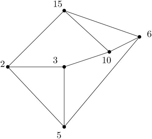
Example 3.8.

The cozero-divisor graph $\Gamma \prime ({\mathbb{Z}}_{30})$ is shown in Figure 1.

By Lemma 3.6, note that $\Gamma \prime ({\mathbb{Z}}_{30})=\Upsilon {\prime }_{30}[\Gamma \prime ({\mathcal{A}}_2),\Gamma \prime ({\mathcal{A}}_3),\Gamma \prime ({\mathcal{A}}_5),\Gamma \prime ({\mathcal{A}}_6),\Gamma \prime ({\mathcal{A}}_{10}),\Gamma \prime ({\mathcal{A}}_{15})],$ where $\Upsilon {\prime }_{30}$ is shown in Figure 2 and $\Gamma \prime ({\mathcal{A}}_2)={\overline{K}}_8,\Gamma \prime ({\mathcal{A}}_3)={\overline{K}}_4=\Gamma \prime ({\mathcal{A}}_6),\Gamma \prime ({\mathcal{A}}_5)={\overline{K}}_2=\Gamma \prime ({\mathcal{A}}_{10}),\Gamma \prime ({\mathcal{A}}_{15})={\overline{K}}_1.$

Figure 1. The graph $\Gamma \prime ({\mathbb{Z}}_{30}).$

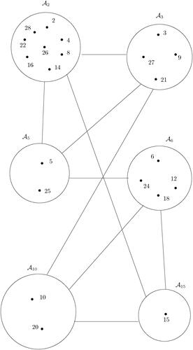
Figure 2. The graph $\Upsilon {\prime }_{3}0.$

4. Laplacian spectrum of $\Gamma \prime ({\mathbb{Z}}_n)$

In this section, we investigate the Laplacian spectrum of the $\Gamma \prime ({\mathbb{Z}}_n)$ for various n. Consider $d_1,d_2,\dots ,d_k$ as all the proper divisors of n. For $1\le i\le k,$ we give the weight $\varphi \left(\frac{n}{d_i}\right)=\left|{\mathcal{A}}_{d_i}\right|$ to the vertex d_i of the graph $\Upsilon {\prime }_n.$ Define the integer $$D_{d_j}=\sum _{d_i\in N_{\Upsilon {\prime }_n}(d_j)}\varphi \left(\frac{n}{d_i}\right)$$ The k × k  weighted Laplacian matrix $L(\Upsilon {\prime }_n)$ of $\Upsilon {\prime }_n$ defined in Theorem 2.1 is given by (3) $$L(\Upsilon {\prime }_n)=\left[\begin{array}{cccc}{D}_{d_1}& -l_{1,2}& \cdots & -l_{1,k}\\ -l_{2,1}& D_{d_2}& \cdots & -l_{2,k}\\ \cdots & \cdots & \cdots & \cdots \\ -l_{k,1}& -l_{k,2}& \cdots & D_{d_k}\end{array}\right]$$(3) where $$l_{i,j}=\{\begin{array}{cc}\varphi \left(\frac{n}{d_j}\right)\hfill & \text{if} d_i\sim d_j \text{in} \Upsilon {\prime }_n;\hfill \\ 0\hfill & \text{otherwise}.\hfill \end{array}$$

Theorem 4.1.

The Laplacian spectrum of $\Gamma \prime ({\mathbb{Z}}_n)$ is given by ${\Phi }_L(\Gamma \prime ({\mathbb{Z}}_n))={\cup }_{i=1}^k(D_{d_i}+({\Phi }_L(\Gamma \prime ({\mathcal{A}}_{d_i}))\setminus \left\{0\right\}))\cup \Phi (L(\Upsilon {\prime }_n)),$ where $D_{d_i}+({\Phi }_L(\Gamma \prime ({\mathcal{A}}_{d_i}))\setminus \{0\})$ represents that $D_{d_i}$ is added to each element of the multiset $({\Phi }_L(\Gamma \prime ({\mathcal{A}}_{d_i}))\setminus \{0\}).$

Proof.

By Lemma 3.6, $\Gamma \prime ({\mathbb{Z}}_n)=\Upsilon {\prime }_n[\Gamma \prime ({\mathcal{A}}_{d_1}),\Gamma \prime ({\mathcal{A}}_{d_2}),\dots ,\Gamma \prime ({\mathcal{A}}_{d_k})].$ Consequently, by Theorem 2.1 and Remark 2.2, the result holds. □

If $n=p^t,$ where t > 1, then the graph $\Gamma \prime ({\mathbb{Z}}_n)$ is a null graph. Let $n\ne p^t$ for any $t\in \mathbb{N}.$ Then by Lemma 3.5, $\Upsilon {\prime }_n$ is connected graph so that $D_{d_i}>0.$ By Theorem 4.1, out of $n-\varphi (n)-1$ Laplacian eigenvalues of $\Gamma \prime ({\mathbb{Z}}_n)$ note that $n-\varphi (n)-1-k$ eigenvalues are non-zero integers. The remaining k Laplacian eigenvalues of $\Gamma \prime ({\mathbb{Z}}_n)$ are the roots of the characteristic equation of the matrix $L(\Upsilon {\prime }_n)$ given in equation (3).

Lemma 4.2.

Let n = pq be a product of two distinct primes. Then the Laplacian spectrum of $\Gamma \prime ({\mathbb{Z}}_n)$ is given by $$\left(\begin{array}{cccc}0& p+q-2& p-1& q-1\\ 1& 1& q-2& p-2\end{array}\right).$$

Proof.

By Lemma 3.6, we have $\Gamma \prime ({\mathbb{Z}}_{pq})=\Upsilon {\prime }_{pq}[\Gamma \prime ({\mathcal{A}}_p),\Gamma \prime ({\mathcal{A}}_q)],$ where $\Upsilon {\prime }_{pq}=K_2,\Gamma \prime ({\mathcal{A}}_p)={\overline{K}}_{\varphi (q)}$ and $\Gamma \prime ({\mathcal{A}}_q)={\overline{K}}_{\varphi (p)}$ (cf. Lemma 3.2 and Corollary 3.4). Consequently, by Theorem 4.1, the Laplacian spectrum of $\Gamma \prime ({\mathbb{Z}}_{pq})$ is $$\begin{array}{cc}{\Phi }_L(\Gamma \prime ({\mathbb{Z}}_{pq}))\hfill & =(D_p+({\Phi }_L(\Gamma \prime ({\mathcal{A}}_p))\setminus \left\{0\right\}))\hfill \\ \hfill & \cup (D_q+({\Phi }_L(\Gamma \prime ({\mathcal{A}}_q))\setminus \left\{0\right\}))\cup \Phi (L(\Upsilon {\prime }_{pq}))\hfill \\ \hfill & =\left(\begin{array}{cc}p-1& q-1\\ q-2& p-2\end{array}\right)\cup \Phi (L(\Upsilon {\prime }_{pq})).\hfill \end{array}$$

Then the matrix $$L(\Upsilon {\prime }_{pq})=\left[\begin{array}{cc}p-1& -(p-1)\\ -(q-1)& q-1\end{array}\right]$$ has eigenvalues $p+q-2$ and 0. Thus, we have the result. □

Notations 4.3.

${({\lambda }_i)}^{[{\mu }_i]}$ denotes the eigenvalue λ_i of $\mathcal{L}(\Gamma \prime ({\mathbb{Z}}_n))$ with multiplicity μ_i.

Lemma 4.4.

For distinct primes p and q, if $n=p^{2}q$ then the Laplacian eigenvalues of $\Gamma \prime ({\mathbb{Z}}_n)$ consists of the set $\left\{{(p^2-p)}^{[(p-1)(q-1)-1]},{(pq-p)}^{[p^2-p-1]},{(p^2-1)}^{[q-2]},{(q-1)}^{[p-2]}\right\}$ and the remaining eigenvalues are the roots of the characteristic polynomial $$\begin{array}{l}{x}^4-\{(p-1)(2p+1)+(p+1)(q-1)\}{x}^3+\{p{(p-1)}^2(p+1)\\ +(p-1){(p+1)}^2(q-1)+p{(q-1)}^2+{(p-1)}^2(q-1)\}{x}^2\\ -p(p-1)(q-1)\{(p-1)(p+1)+p(q-1)\}x.\end{array}$$

Proof.

First note that $\Upsilon {\prime }_{p^{2}q}$ is the path graph given by $p\sim q\sim p^2\sim pq.$ By Lemma 3.6, $$\Gamma \prime ({\mathbb{Z}}_{p^{2}q})=\Upsilon {\prime }_{p^{2}q}[\Gamma \prime ({\mathcal{A}}_p),\Gamma \prime ({\mathcal{A}}_q),\Gamma \prime ({\mathcal{A}}_{p^2}),\Gamma \prime ({\mathcal{A}}_{pq})],$$ where $\Gamma \prime ({\mathcal{A}}_p)={\overline{K}}_{\varphi (pq)},\Gamma \prime ({\mathcal{A}}_q)={\overline{K}}_{\varphi (p^2)},\Gamma \prime ({\mathcal{A}}_{p^2})={\overline{K}}_{\varphi (q)}$ and $\Gamma \prime ({\mathcal{A}}_{pq})={\overline{K}}_{\varphi (p)}.$ It follows that $D_p=\varphi (p^2)=p^2-p$ and $D_q=\varphi (pq)+\varphi (q)=p(q-1),D_{p^2}=\varphi (p^2)+\varphi (p)=p^2-1$ and $D_{pq}=\varphi (q)=q-1.$ Therefore, by Theorem 4.1, the Laplacian spectrum of $\Gamma \prime ({\mathbb{Z}}_{p^{2}q})$ is $$\begin{array}{ll}{\Phi }_L(\Gamma \prime ({\mathbb{Z}}_{p^{2}q}))\hfill & =(D_p+({\Phi }_L(\Gamma \prime ({\mathcal{A}}_p))\setminus \left\{0\right\}))\cup (D_q+({\Phi }_L(\Gamma \prime ({\mathcal{A}}_q))\setminus \left\{0\right\}))\cup (D_{p^2}+({\Phi }_L(\Gamma \prime ({\mathcal{A}}_{p^2}))\setminus \left\{0\right\}))\hfill \\ \hfill & \cup (D_{pq}+({\Phi }_L(\Gamma \prime ({\mathcal{A}}_{pq}))\setminus \left\{0\right\}))\cup \Phi (L(\Upsilon {\prime }_{p^{2}q}))\hfill \\ \hfill & =\left(\begin{array}{cccc}{p}^2-p& pq-p& p^2-1& q-1\\ (p-1)(q-1)-1& p^2-p-1& q-2& p-2\end{array}\right)\cup \Phi (L(\Upsilon {\prime }_{p^{2}q})).\hfill \end{array}$$

Thus, the remaining Laplacian eigenvalues can be obtained by the characteristic polynomial (given in the statement) of the matrix $$L(\Upsilon {\prime }_{p^{2}q})=\left[\begin{array}{cccc}{p}^2-p& -p^2+p& 0& 0\\ -(p-1)(q-1)& p(q-1)& -(q-1)& 0\\ 0& -p^2+p& p^2-1& -p+1\\ 0& 0& -q+1& q-1\end{array}\right].$$

□

Lemma 4.5.

For distinct primes p and q, if $n=p^{n_1}q$ then the Laplacian eigenvalues of $\Gamma \prime ({\mathbb{Z}}_n)$ consists of the set $\{{(\varphi (p^{n_1}))}^{[\varphi (p^{n_1-1}q)-1]},{(\varphi (p^{n_1})+\varphi (p^{n_1-1}))}^{[\varphi (p^{n_1-2}q)-1]},{({\sum }_{i=0}^2\varphi (p^{n_1-i}))}^{[\varphi (p^{n_1-3}q)-1]},\dots ,{({\sum }_{i=0}^{n_1-1}\varphi (p^{n_1-i}))}^{[\varphi (p^{n_1-n_1}q)-1]},{({\sum }_{i=1}^{n_1}\varphi (p^{n_1-i}q))}^{[\varphi (p^{n_1})-1]},{({\sum }_{i=2}^{n_1}\varphi (p^{n_1-i}q))}^{[\varphi (p^{n_1-1})-1]},\dots ,{(\varphi (q))}^{[\varphi (p)-1]}\}$ and the remaining eigenvalues are the eigenvalues of the matrix given in equation (3).

Proof.

Note that $\{p,p^2,\dots ,p^{n_1},q,pq,p^{2}q,\dots ,p^{n_1-1}q\}$ is the vertex set of the graph $\Upsilon {\prime }_{p^{n_1}q}.$ By Lemma 3.6, $$\Gamma \prime ({\mathbb{Z}}_{p^{n_1}q})=\Upsilon {\prime }_{p^{n_1}q}[\Gamma \prime ({\mathcal{A}}_p),\Gamma \prime ({\mathcal{A}}_{p^2}),\dots ,\Gamma \prime ({\mathcal{A}}_{p^{n_1}}),\Gamma \prime ({\mathcal{A}}_q),\Gamma \prime ({\mathcal{A}}_{pq}),\Gamma \prime ({\mathcal{A}}_{p^{2}q}),\dots ,\Gamma \prime ({\mathcal{A}}_{p^{n_1-1}q})],$$ where, $\Gamma \prime ({\mathcal{A}}_p)={\overline{K}}_{\varphi (p^{n_1-1}q)},\Gamma \prime ({\mathcal{A}}_{p^2})={\overline{K}}_{\varphi (p^{n_1-2}q)},\cdots ,\Gamma \prime ({\mathcal{A}}_{p^{n_1}})={\overline{K}}_{\varphi (q)},\Gamma \prime ({\mathcal{A}}_q)={\overline{K}}_{\varphi (p^{n_1})},\Gamma \prime ({\mathcal{A}}_{pq})={\overline{K}}_{\varphi (p^{n_1-1})},\cdots ,\Gamma \prime ({\mathcal{A}}_{p^{n_1-1}q})={\overline{K}}_{\varphi (p)}.$ It follows that $D_p=\varphi (p^{n_1}),D_{p^2}=\varphi (p^{n_1})+\varphi (p^{n_1-1}),\cdots ,D_{p^{n_1}}={\sum }_{i=0}^{n_1-1}\varphi (p^{n_1-i}),D_q={\sum }_{i=1}^{n_1}\varphi (p^{n_1-i}q),D_{pq}={\sum }_{i=2}^{n_1}\varphi (p^{n_1-i}q),\cdots ,D_{p^{n_1-1}q}=\varphi (q).$ Consequently, by Theorem 4.1, the Laplacian spectrum of $\Gamma \prime ({\mathbb{Z}}_{p^{n_1}q})$ is $$\begin{array}{cc}{\Phi }_L(\Gamma \prime ({\mathbb{Z}}_{p^{n_1}q}))\hfill & =(D_p+({\Phi }_L(\Gamma \prime ({\mathcal{A}}_p))\setminus \left\{0\right\}))\cup (D_{p^2}+({\Phi }_L(\Gamma \prime ({\mathcal{A}}_{p^2}))\setminus \left\{0\right\}))\cup \cdots \cup (D_{p^{n_1}}+({\Phi }_L(\Gamma \prime ({\mathcal{A}}_{p^{n_1}}))\setminus \left\{0\right\}))\hfill \\ \hfill & \cup (D_q+({\Phi }_L(\Gamma \prime ({\mathcal{A}}_q))\setminus \left\{0\right\}))\cup (D_{pq}+({\Phi }_L(\Gamma \prime ({\mathcal{A}}_{pq}))\setminus \left\{0\right\}))\cup \cdots \cup (D_{p^{n_1-1}q}+({\Phi }_L(\Gamma \prime ({\mathcal{A}}_{p^{n_1-1}q}))\setminus \left\{0\right\}))\hfill \\ \hfill & \cup \Phi (L(\Upsilon {\prime }_{p^{n_1}q})).\hfill \\ \hfill & =\left(\begin{array}{ccccccc}\varphi (p^{n_1})& \cdots & \sum _{i=0}^{n_1-1}\varphi (p^{n_1-i})& \sum _{i=1}^{n_1}\varphi (p^{n_1-i}q)& \sum _{i=2}^{n_1}\varphi (p^{n_1-i}q)& \cdots & \varphi (q)\\ \varphi (p^{n_1-1}q)-1& \cdots & \varphi (p^{n_1-n_1}q)-1& \varphi (p^{n_1})-1& \varphi (p^{n_1})-1& \cdots & \varphi (p)-1\end{array}\right)\cup \Phi (L(\Upsilon {\prime }_{p^{n_1}q})).\hfill \end{array}$$

Thus, the remaining $2n_1$ Laplacian eigenvalues are the eigenvalues of the matrix $L(\Upsilon {\prime }_{p^{n_1}q})=$ $$\left[\begin{array}{ccccccccc}\varphi (p^{n_1})& 0& 0& \cdots & 0& \cdots & \cdots & 0& -\varphi (p^{n_1})\\ 0& \sum _{i=0}^1\varphi (p^{n_1-i})& 0& \cdots & \cdots & 0& \cdots & -\varphi (p^{n_1-1})& -\varphi (p^{n_1})\\ ⋮& ⋮& ⋮& ⋮& ⋮& ⋮& ⋮& ⋮& ⋮\\ 0& 0& 0& \cdots & \sum _{i=0}^{n_1-1}\varphi (p^{n_1-i})& -\varphi (p)& -\varphi (p^2)& \cdots & -\varphi (p^{n_1})\\ 0& 0& 0& \cdots & -\varphi (q)& \varphi (q)& 0& \cdots & 0\\ 0& \cdots & \cdots & -\varphi (pq)& -\varphi (q)& 0& \varphi (pq)+\varphi (q)& \cdots & 0\\ ⋮& ⋮& ⋮& ⋮& ⋮& ⋮& ⋮& ⋮& ⋮\\ -\varphi (p^{n_1-1}q)& -\varphi (p^{n_1-2}q)& \cdots & \cdots & -\varphi (q)& 0& 0& \cdots & \sum _{i=1}^{n_1}\varphi (p^{n_1-i}q)\end{array}\right]$$ where matrix $L(\Upsilon {\prime }_{p^{n_1}q})$ is obtained by indexing the rows and columns as $p,p^2,\dots ,p^{n_1},p^{n_1-1}q,\dots ,pq,q.$ □

Theorem 4.6.

If $n=p^{n_1}{q}^{n_2}$, where p and q are distinct primes. Then the set of Laplacian eigenvalues of $\Gamma \prime ({\mathbb{Z}}_n)$ consists of $$\begin{array}{c}\begin{array}{c}{\left(\sum _{i=1}^{n_2}\varphi (p^{n_1}{q}^{n_2-i})\right)}^{[\varphi (p^{n_1-1}{q}^{n_2})-1]}, {\left(\sum _{i=1}^{n_2}\varphi (p^{n_1}{q}^{n_2-i})+\sum _{i=1}^{n_2}\varphi (p^{n_1-1}{q}^{n_2-i})\right)}^{[\varphi (p^{n_1-2}{q}^{n_2})-1]},\hfill \\ {\left(\sum _{i=1}^{n_2}\varphi (p^{n_1}{q}^{n_2-i})+\sum _{i=1}^{n_2}\varphi (p^{n_1-1}{q}^{n_2-i})+\sum _{i=1}^{n_2}\varphi (p^{n_1-2}{q}^{n_2-i})\right)}^{[\varphi (p^{n_1-3}{q}^{n_2})-1]},\hfill \\ ⋮\hfill \\ {\left(\sum _{i=1}^{n_2}\varphi (p^{n_1}{q}^{n_2-i})+\sum _{i=1}^{n_2}\varphi (p^{n_1-1}{q}^{n_2-i})+\cdots +\sum _{i=1}^{n_2}\varphi (p{q}^{n_2-i})\right)}^{[\varphi (q^{n_2})-1]},\hfill \end{array}\\ \begin{array}{c}{\left(\sum _{i=1}^{n_1}\varphi (p^{n_1-i}{q}^{n_2})\right)}^{[\varphi (p^{n_1}{q}^{n_2-1})-1]},{\left(\sum _{i=1}^{n_1}\varphi (p^{n_1-i}{q}^{n_2})+\sum _{i=1}^{n_1}\varphi (p^{n_1-i}{q}^{n_2-1})\right)}^{[\varphi (p^{n_1}{q}^{n_2-2})-1]},\hfill \\ {\left(\sum _{i=1}^{n_1}\varphi (p^{n_1-i}{q}^{n_2})+\sum _{i=1}^{n_1}\varphi (p^{n_1-i}{q}^{n_2-1})+\sum _{i=1}^{n_1}\varphi (p^{n_1-i}{q}^{n_2-2})\right)}^{[\varphi (p^{n_1}{q}^{n_2-3})-1]},\hfill \\ ⋮\hfill \\ {\left(\sum _{i=1}^{n_1}\varphi (p^{n_1-i}{q}^{n_2})+\sum _{i=1}^{n_1}\varphi (p^{n_1-i}{q}^{n_2-1})+\cdots +\sum _{i=1}^{n_1}\varphi (p^{n_1-i}q)\right)}^{[\varphi (p^{n_1})-1]},\hfill \\ {\left(\sum _{i=2}^{n_1}\varphi (p^{n_1-i}{q}^{n_2})+\sum _{i=2}^{n_2}\varphi (p^{n_1}{q}^{n_2-i})\right)}^{[\varphi (p^{n_1-1}{q}^{n_2-1})-1]},\hfill \end{array}\\ \begin{array}{c}{\left(\sum _{i=3}^{n_1}\varphi (p^{n_1-i}{q}^{n_2})+\sum _{i=2}^{n_2}\varphi (p^{n_1}{q}^{n_2-i})+\sum _{i=1}^{n_2}\varphi (p^{n_1-1}{q}^{n_2-i})\right)}^{[\varphi (p^{n_1-2}{q}^{n_2-1})-1]},\hfill \\ ⋮\hfill \\ {\left(\sum _{i=2}^{n_2}\varphi (p^{n_1}{q}^{n_2-i})+\sum _{i=1}^{n_1}\varphi (p^{n_1-i}{q}^{n_2-2})+\sum _{i=1}^{n_1}\varphi (p^{n_1-i}{q}^{n_2-3})+\cdots +\sum _{i=1}^{n_1-1}\varphi (p^{n_1-i})\right)}^{[\varphi (q^{n_2-1})-1]},\hfill \\ {\left(\sum _{i=2}^{n_1}\varphi (p^{n_1-i}{q}^{n_2})+\sum _{i=3}^{n_2}\varphi (p^{n_1}{q}^{n_2-i})+\sum _{i=2}^{n_1}\varphi (p^{n_1-i}{q}^{n_2-1})\right)}^{[\varphi (p^{n_1-1}{q}^{n_2-2})-1]},\hfill \\ ⋮\hfill \\ {\left(\sum _{i=2}^{n_1}\varphi (p^{n_1-i}{q}^{n_2})+\sum _{i=1}^{n_2}\varphi (p^{n_1-2}{q}^{n_2-i})+\sum _{i=1}^{n_2}\varphi (p^{n_1-3}{q}^{n_2-i})+\cdots +\sum _{i=1}^{n_2-1}\varphi (q^{n_2-i})\right)}^{[\varphi (p^{n_1-1})-1]},\hfill \\ ⋮\hfill \\ {\left(\sum _{i=1}^{n_2-1}\varphi (q^{n_2-i})+\varphi (q^{n_2})\right)}^{[\varphi (p)-1]}\hfill \end{array}\end{array}$$ and the remaining $(n_1+1)(n_2+1)-2$ eigenvalues are given by the zeros of the characteristic polynomial of the matrix given in equation (3).

Proof.

The set of proper divisors of $n=p^{n_1}{q}^{n_2}$ is $$\{p,p^2,\dots ,p^{n_1},q,q^2,\dots ,q^{n_2},pq,p^{2}q,\dots ,p^{n_1}q,p{q}^2,p^2{q}^2,\dots ,p^{n_1}{q}^2,\cdots ,p{q}^{n_2},p^2{q}^{n_2},\dots ,p^{n_1-1}{q}^{n_2}\}.$$

By the definition of $\Upsilon {\prime }_n,$ note that

• $p^i\sim q^j$ for all i, j.

• $p^i\sim p^{i_1}{q}^{j_1}$ for $i>i_1$ and $j_1>0.$

• $q^j\sim p^i{q}^{j_1}$ for $j>j_1$ and i > 0.

• If either $i_1>i_2,j_1<j_2$ or $j_1>j_2,i_1<i_2,$ then $p^{i_1}{q}^{j_1}\sim p^{i_2}{q}^{j_2}.$

In view of Lemma 3.6, $$\begin{array}{c}\Gamma \prime ({\mathbb{Z}}_{p^{n_1}{q}^{n_2}})=\Upsilon {\prime }_{p^{n_1}{q}^{n_2}}[\Gamma \prime ({\mathcal{A}}_p),\Gamma \prime ({\mathcal{A}}_{p^2}),\dots ,\Gamma \prime ({\mathcal{A}}_{p^{n_1}}),\Gamma \prime ({\mathcal{A}}_q),\Gamma \prime ({\mathcal{A}}_{q^2}),\dots ,\Gamma \prime ({\mathcal{A}}_{q^{n_2}}),\Gamma \prime ({\mathcal{A}}_{pq}),\Gamma \prime ({\mathcal{A}}_{p^{2}q}),\dots ,\Gamma \prime ({\mathcal{A}}_{p^{n_1}q}),\\ \cdots ,\Gamma \prime ({\mathcal{A}}_{p{q}^{n_2}}),\dots ,\Gamma \prime ({\mathcal{A}}_{p^{n_1-1}{q}^{n_2}})].\end{array}$$

Therefore, by Lemma 3.2 and Corollary 3.4, we get

$\Gamma \prime ({\mathcal{A}}_{p^i})={\overline{K}}_{\varphi (p^{n_1-i}{q}^{n_2})},$ where $1\le i\le n_1,$

$\Gamma \prime ({\mathcal{A}}_{q^j})={\overline{K}}_{\varphi (p^{n_1}{q}^{n_2-j})}$ where $1\le j\le n_2,$

$\Gamma \prime ({\mathcal{A}}_{p^i{q}^j})={\overline{K}}_{\varphi (p^{n_1-i}{q}^{n_2-j})}.$

Consequently, we have $$\begin{array}{c}\begin{array}{c}{D}_p=\sum _{i=1}^{n_2}\varphi (p^{n_1}{q}^{n_2-i}),D_{p^2}=\sum _{i=1}^{n_2}\varphi (p^{n_1}{q}^{n_2-i})+\sum _{i=1}^{n_2}\varphi (p^{n_1-1}{q}^{n_2-i}),\hfill \\ ⋮\hfill \\ D_{p^{n_1}}=\sum _{i=1}^{n_2}\varphi (p^{n_1}{q}^{n_2-i})+\sum _{i=1}^{n_2}\varphi (p^{n_1-1}{q}^{n_2-i})+\cdots +\sum _{i=1}^{n_2}\varphi (p{q}^{n_2-i}),\hfill \\ D_q=\sum _{i=1}^{n_1}\varphi (p^{n_1-i}{q}^{n_2}),\hfill \\ ⋮\hfill \\ D_{q^{n_2}}=\sum _{i=1}^{n_1}\varphi (p^{n_1-i}{q}^{n_2})+\sum _{i=1}^{n_1}\varphi (p^{n_1-i}{q}^{n_2-1})+\cdots +\sum _{i=1}^{n_1}\varphi (p^{n_1-i}q),D_{pq}=\sum _{i=2}^{n_1}\varphi (p^{n_1-i}{q}^{n_2})+\sum _{i=2}^{n_2}\varphi (p^{n_1}{q}^{n_2-i}),\hfill \\ ⋮\hfill \end{array}\\ \begin{array}{l}{D}_{p^{n_1}q}=\sum _{i=2}^{n_2}\varphi (p^{n_1}{q}^{n_2-i})+\sum _{i=1}^{n_1}\varphi (p^{n_1-i}{q}^{n_2-2})+\sum _{i=1}^{n_1}\varphi (p^{n_1-i}{q}^{n_2-3})+\cdots +\sum _{i=1}^{n_1-1}\varphi (p^{n_1-i}),\hfill \\ D_{p{q}^2}=\sum _{i=2}^{n_1}\varphi (p^{n_1-i}{q}^{n_2})+\sum _{i=3}^{n_2}\varphi (p^{n_1}{q}^{n_2-i})+\sum _{i=2}^{n_1}\varphi (p^{n_1-i}{q}^{n_2-1}),\hfill \\ ⋮\hfill \\ D_{p{q}^{n_2}}=\sum _{i=2}^{n_1}\varphi (p^{n_1-i}{q}^{n_2})+\sum _{i=1}^{n_2}\varphi (p^{n_1-2}{q}^{n_2-i})+\sum _{i=1}^{n_2}\varphi (p^{n_1-3}{q}^{n_2-i})+\cdots +\sum _{i=1}^{n_2-1}\varphi (q^{n_2-i}),\hfill \\ ⋮\hfill \\ D_{p^{n_1-1}{q}^{n_2}}=\sum _{i=1}^{n_2-1}\varphi (q^{n_2-i})+\varphi (q^{n_2}).\hfill \end{array}\end{array}$$

Therefore, by Theorem 4.1, the Laplacian spectrum of $\Gamma \prime ({\mathbb{Z}}_{p^{n_1}{q}^{n_2}})$ is $$\begin{array}{cc}{\Phi }_L(\Gamma \prime ({\mathbb{Z}}_{p^{n_1}{q}^{n_2}}))\hfill & =(D_p+({\Phi }_L(\Gamma \prime ({\mathcal{A}}_p))\setminus \left\{0\right\}))\cup (D_{p^2}+({\Phi }_L(\Gamma \prime ({\mathcal{A}}_{p^2}))\setminus \left\{0\right\}))\cup \cdots \cup (D_{p^{n_1}}+({\Phi }_L(\Gamma \prime ({\mathcal{A}}_{p^{n_1}}))\setminus \left\{0\right\}))\hfill \\ \hfill & \cup (D_q+({\Phi }_L(\Gamma \prime ({\mathcal{A}}_q))\setminus \left\{0\right\}))\cup (D_{q^2}+({\Phi }_L(\Gamma \prime ({\mathcal{A}}_{q^2}))\setminus \left\{0\right\}))\cup \cdots \cup (D_{q^{n_2}}+({\Phi }_L(\Gamma \prime ({\mathcal{A}}_{q^{n_2}}))\setminus \left\{0\right\}))\hfill \\ \hfill & \cup (D_{pq}+({\Phi }_L(\Gamma \prime ({\mathcal{A}}_{pq}))\setminus \left\{0\right\}))\cup \cdots \cup (D_{p^{n_1}q}+({\Phi }_L(\Gamma \prime ({\mathcal{A}}_{p^{n_1}q}))\setminus \left\{0\right\}))\cup \cdots \hfill \\ \hfill & \cup (D_{p{q}^{n_2}}+({\Phi }_L(\Gamma \prime ({\mathcal{A}}_{p{q}^{n_2}}))\setminus \left\{0\right\}))\cup \cdots \cup (D_{p^{n_1-1}{q}^{n_2}}+({\Phi }_L(\Gamma \prime ({\mathcal{A}}_{p^{n_1-1}{q}^{n_2}}))\setminus \left\{0\right\}))\cup \Phi (L(\Upsilon {\prime }_{p^{n_1}{q}^{n_2}})).\hfill \end{array}$$

The remaining $(n_1+1)(n_2+1)-2$ eigenvalues are the zeros of the characteristic polynomial of the matrix $L(\Upsilon {\prime }_{p^{n_1}{q}^{n_2}})$ given in equation (3). □

5. The Laplacian spectral radius and the algebraic connectivity of $\Gamma \prime ({\mathbb{Z}}_n)$

In this section, we study the algebraic connectivity and the Laplacian spectral radius of $\Gamma \prime ({\mathbb{Z}}_n).$ We obtain all those values of n for which the Laplacian spectral radius of $\Gamma \prime ({\mathbb{Z}}_n)$ is equal to order of $\Gamma \prime ({\mathbb{Z}}_n).$ Moreover, the values of n for which the algebraic connectivity and the vertex connectivity coincide are also described. The following theorem follows from the relation $\lambda (\Gamma )=|V(\Gamma )|-\mu (\overline{\Gamma })$ and the fact $\overline{\Gamma }$ is disconnected if and only if Γ is the join of two graphs.

Theorem 5.1

([13]). If Γ is a graph on m vertices, then $\lambda (\Gamma )\le m$. Further, equality holds if and only if $\overline{\Gamma }$ is disconnected if and only if Γ is the join of two graphs.

In view of Theorem 5.1, first we characterize the values of n for which the complement of $\Gamma \prime ({\mathbb{Z}}_n)$ is disconnected.

Proposition 5.2.

$\overline{\Gamma \prime ({\mathbb{Z}}_n)}$ is disconnected if and only if n is a product of two distinct primes.

Proof.

Let p and q be two distinct primes. If n = pq, then by Remark 3.1 we get $V(\Gamma \prime ({\mathbb{Z}}_n))={\mathcal{A}}_p\cup {\mathcal{A}}_q$ such that ${\mathcal{A}}_p\cap {\mathcal{A}}_q=\varnothing .$ In fact, $\Gamma \prime ({\mathbb{Z}}_n)=K_{\varphi (q),\varphi (p)}$ is a complete bipartite graph. Consequently, $\overline{\Gamma \prime ({\mathbb{Z}}_n)}$ is a disconnected graph.

Conversely, suppose $\overline{\Gamma \prime ({\mathbb{Z}}_n)}$ is disconnected. Clearly, for n = p  there is nothing to prove. If $n=p^{\alpha }$ for some $1<\alpha \in \mathbb{N},$ then $\Gamma \prime ({\mathbb{Z}}_{p^{\alpha }})$ is a null graph. Consequently, $\overline{\Gamma \prime ({\mathbb{Z}}_{p^{\alpha }})}$ is a complete graph which is not possible. If possible, let $n\ne pq.$ Let d₁ and d₂ be the proper divisors of n and let $x\in {\mathcal{A}}_{d_1},y\in {\mathcal{A}}_{d_2}.$ If d₁ = d₂ then clearly $x\sim y$ in $\overline{\Gamma \prime ({\mathbb{Z}}_n)}.$ If $d_1\ne d_2$ such that either $d_1|d_2$ or $d_2|d_1$ then $x\sim y$ in $\overline{\Gamma \prime ({\mathbb{Z}}_n)}$ (cf. Lemma 3.3). If $d_1\ne d_2$ and neither $d_1|d_2$ nor $d_2|d_1,$ then there exist two primes p₁ and p₂ such that $p_1|d_1$ and $p_2|d_2.$ Consequently, $x\sim z_1\sim z_2\sim z_3\sim y$ in $\overline{\Gamma \prime ({\mathbb{Z}}_n)}$ for some $z_1\in {\mathcal{A}}_{p_1},z_2\in {\mathcal{A}}_{p_1{p}_2}$ and $z_3\in {\mathcal{A}}_{p_2}.$ Thus, $\overline{\Gamma \prime ({\mathbb{Z}}_n)}$ is connected; a contradiction. Hence, n must be a product of two distinct primes. □

Since $|V(\Gamma \prime ({\mathbb{Z}}_n))|=n-\varphi (n)-1,$ by using the Proposition 5.2 in Theorem 5.1, we have the following proposition.

Proposition 5.3.

$\lambda (\Gamma \prime ({\mathbb{Z}}_n))=|V(\Gamma \prime ({\mathbb{Z}}_n))|$ if and only if n is a product of two distinct primes. Moreover, if n = pq then $\lambda (\Gamma \prime ({\mathbb{Z}}_n))=p+q-2.$

Now we classify all those values of n for which the algebraic connectivity and the vertex connectivity of $\Gamma \prime ({\mathbb{Z}}_n)$ are equal. The following theorem is useful in this study.

Theorem 5.4.

[15] Let Γ be a non-complete connected graph on m vertices. Then $\kappa (\Gamma )=\mu (\Gamma )$ if and only if Γ can be written as ${\Gamma }_1\vee {\Gamma }_2$, where ${\Gamma }_1$ is a disconnected graph on $m-\kappa (\Gamma )$ vertices and ${\Gamma }_2$ is a graph on $\kappa (\Gamma )$ vertices with $\mu ({\Gamma }_2)\ge 2\kappa (\Gamma )-m.$

Lemma 5.5.

For distinct primes p and q, if n = pq where p < q then $\kappa (\Gamma \prime ({\mathbb{Z}}_n))=\delta (\Gamma \prime ({\mathbb{Z}}_n))=p-1.$

Proof.

For n = pq, $\Gamma \prime ({\mathbb{Z}}_n)$ is a complete bipartite graph with partition sets ${\mathcal{A}}_p$ and ${\mathcal{A}}_q.$ Hence, $\kappa (\Gamma \prime ({\mathbb{Z}}_n))=\delta (\Gamma \prime ({\mathbb{Z}}_n))=\text{min}\left\{\right|{\mathcal{A}}_p|,|{\mathcal{A}}_q\left|\right\}=p-1$ □

Theorem 5.6.

For the graph $\Gamma \prime ({\mathbb{Z}}_n)$, we have $\mu (\Gamma \prime ({\mathbb{Z}}_n))\le \kappa (\Gamma \prime ({\mathbb{Z}}_n))$. The equality holds if and only if n is a product of two distinct primes.

Proof.

By [15], for any graph Γ which is not complete, we have $\mu (\Gamma )\le \kappa (\Gamma ).$ If n = 4 then there is nothing to prove because $\Gamma \prime ({\mathbb{Z}}_4)$ is the graph of one vertex only. If $n\ne 4$ then $\Gamma \prime ({\mathbb{Z}}_n)$ is not a complete graph. Consequently, $\mu (\Gamma \prime ({\mathbb{Z}}_n))\le \kappa (\Gamma \prime ({\mathbb{Z}}_n)).$

If n is not a product of two distinct primes then by Proposition 5.2 and by Theorem 5.1, $\Gamma \prime ({\mathbb{Z}}_n)$ cannot be written as the join of two graphs. Thus, by Theorem 5.4, we obtain $\mu (\Gamma \prime ({\mathbb{Z}}_n))<\kappa (\Gamma \prime ({\mathbb{Z}}_n)).$ If n = pq, where p and q are distinct primes such that p <q  , then by Theorem 5.1, Proposition 5.2, Theorem 5.4 and Lemma 5.5, we obtain $\mu (\Gamma \prime ({\mathbb{Z}}_n))=\kappa (\Gamma \prime ({\mathbb{Z}}_n))=p-1.$ □

6. The Wiener index of $\Gamma \prime ({\mathbb{Z}}_n)$

In this section, we obtain the Wiener index of the cozero-divisor graph of the ring ${\mathbb{Z}}_n$ for arbitrary $n\in \mathbb{N}.$ Consequently, we obtain the diameter of $\Gamma \prime ({\mathbb{Z}}_n)$ (see Proposition 6.4). For a prime p and $1\le \alpha \in \mathbb{N},$ the graph $\Gamma \prime ({\mathbb{Z}}_p)$ is empty whereas $\Gamma \prime ({\mathbb{Z}}_{p^{\alpha }})$ is a null graph. Therefore $W(\Gamma \prime ({\mathbb{Z}}_p))=W(\Gamma \prime ({\mathbb{Z}}_{p^{\alpha }}))=0.$

Theorem 6.1.

For $1\le i\le \tau (n)-2$, let d_i’s be the proper divisors of n. If $n=p_1{p}_2\cdots p_k$, where p_i’s are distinct primes and $2\le k\in \mathbb{N}$, then $$W(\Gamma \prime ({\mathbb{Z}}_n))=\sum _{i=1}^{2^k-2}\varphi \left(\frac{n}{d_i}\right)\left(\varphi \left(\frac{n}{d_i}\right)-1\right)+\frac{1}{2}\sum _{\begin{array}{c}{d}_i\nmid d_j\\ d_j\nmid d_i\end{array}}\varphi \left(\frac{n}{d_i}\right)\varphi \left(\frac{n}{d_j}\right)+2\sum _{\begin{array}{c}{d}_i|d_j\\ i\ne j\end{array}}\varphi \left(\frac{n}{d_i}\right)\varphi \left(\frac{n}{d_j}\right).$$

Proof.

To determine the Wiener index of $\Gamma \prime ({\mathbb{Z}}_n),$ we first obtain the distances between the vertices of each ${\mathcal{A}}_{d_i}$ and two distinct ${\mathcal{A}}_{d_i}$’s, respectively. For a proper divisor d_i of n, let $x,y\in {\mathcal{A}}_{d_i}.$ Since $\Gamma \prime ({\mathbb{Z}}_n)$ is connected, by Corollary 3.4, there exists a proper divisor d_r of n such that $x\sim z$ for each $x\in {\mathcal{A}}_{d_i}$ and $z\in {\mathcal{A}}_{d_r}.$ Consequently, $d(x,y)=2$ for any two distinct $x,y\in {\mathcal{A}}_{d_i}.$ Now we obtain the distances between the vertices of any two distinct ${\mathcal{A}}_{d_i}$’s through the following cases.

Case-1: Neither $d_i|d_j$ nor $d_j|d_i.$ By Lemma 3.3, $d(x,y)=1$ for every $x\in {\mathcal{A}}_{d_i}$ and $y\in {\mathcal{A}}_{d_j}.$

Case-2: $d_i|d_j.$ For $x\in {\mathcal{A}}_{d_i}$ and $y\in {\mathcal{A}}_{d_j}$ we have $x\nsim y.$ Without loss of generality, assume that $d_j=p_1{p}_2\cdots p_m{d}_i,$ where $1\le m\le k-2.$ Since d_j is a proper divisor of n there exists a prime p such that $p\nmid d_j.$ Consequently, $p\nmid d_i.$ It follows that for $x\in {\mathcal{A}}_{d_i}$ and $y\in {\mathcal{A}}_{d_j}$ there exists a $z\in {\mathcal{A}}_p$ such that $x\sim z\sim y.$ Thus, $d(x,y)=2$ for each $x\in {\mathcal{A}}_{d_i}$ and $y\in {\mathcal{A}}_{d_j}.$

Thus, in view of all the possible distances between the vertices of $\Gamma \prime ({\mathbb{Z}}_n),$ we get $$\begin{array}{ll}W(\Gamma \prime ({\mathbb{Z}}_n))\hfill & =\frac{1}{2}\sum _{u\in V(\Gamma \prime ({\mathbb{Z}}_n))}\sum _{v\in V(\Gamma \prime ({\mathbb{Z}}_n))}d(u,v)\hfill \\ \hfill & =\frac{1}{2}[\sum _{i=1}^{2^k-2}2|{\mathcal{A}}_{d_i}|(\left|{\mathcal{A}}_{d_i}\right|-1)+\sum _{\begin{array}{c}{d}_i\nmid d_j\\ d_j\nmid d_i\end{array}}\left|{\mathcal{A}}_{d_i}\right|\left|{\mathcal{A}}_{d_j}\right|]\hfill \\ \hfill & +2\sum _{}\left|{\mathcal{A}}_{d_i}\right|\left|{\mathcal{A}}_{d_j}\right|\hfill \\ \hfill & =\sum _{i=1}^{2^k-2}\varphi (\frac{n}{d_i})(\varphi (\frac{n}{d_i})-1)\hfill \\ \hfill & +\frac{1}{2}\sum _{\begin{array}{c}{d}_i\nmid d_j\\ d_j\nmid d_i\end{array}}\varphi (\frac{n}{d_i})\varphi (\frac{n}{d_j})\hfill \\ \hfill & +2\sum _{\begin{array}{c}{d}_i|d_j\\ i\ne j\end{array}}\varphi (\frac{n}{d_i})\varphi (\frac{n}{d_j}).\hfill \end{array}$$ □

Corollary 6.2.

If n = pq, where p, q are distinct primes, then $W(\Gamma \prime ({\mathbb{Z}}_n))=(p-1)(q-1)+(p-1)(p-2)+(q-1)(q-2).$

Theorem 6.3.

Let $n=p_1^{n_1}{p}_2^{n_2}\cdots p_r^{n_r}\cdots p_k^{n_k}$ with $k\ge 2$, where p_i’s are distinct primes and let $D=\{d_1,d_2,\dots ,d_{\tau (n)-2}\}$ be the set of all proper divisors of n. For $d_i|d_j$, define $$\begin{array}{cc}A\hfill & =\{(d_i,d_j)\in D\times D|d_i\ne p_r^s\};\hfill \\ B\hfill & =\{(d_i,d_j)\in D\times D|d_i=p_r^s\mathit{and}\frac{n}{d_j}\ne p_r^t\};\hfill \\ C\hfill & =\{(d_i,d_j)\in D\times D|d_i=p_r^s\mathit{and}\frac{n}{d_j}=p_r^t\}.\hfill \end{array}$$ Then $$\begin{array}{c}W(\Gamma \prime ({\mathbb{Z}}_n))=\sum _{i=1}^{\tau (n)-2}\varphi \left(\frac{n}{d_i}\right)\left(\varphi \left(\frac{n}{d_i}\right)-1\right)+\frac{1}{2}\sum _{\begin{array}{c}{d}_i\nmid d_j\\ d_j\nmid d_i\end{array}}\varphi \left(\frac{n}{d_i}\right)\varphi \left(\frac{n}{d_j}\right)+2\sum _{(d_i,d_j)\in A}\varphi \left(\frac{n}{d_i}\right)\varphi \left(\frac{n}{d_j}\right)+2\sum _{(d_i,d_j)\in B}\varphi \left(\frac{n}{d_i}\right)\varphi \left(\frac{n}{d_j}\right)\hfill \\ + 3\sum _{(d_i,d_j)\in C}\varphi \left(\frac{n}{d_i}\right)\varphi \left(\frac{n}{d_j}\right).\hfill \end{array}$$

Proof.

In view of Remark 3.1, first we obtain all the possible distances between the vertices of ${\mathcal{A}}_{d_i}$ and ${\mathcal{A}}_{d_j},$ where d_i and d_j are proper divisors of n. If i = j  then by the proof of Theorem 6.1, we get $d(x,y)=2$ for any two distinct $x,y\in {\mathcal{A}}_{d_i}.$ Now suppose that $i\ne j.$ If $d_i\nmid d_j$ and $d_j\nmid d_i,$ then by Lemma 3.3, we get $d(x,y)=1$ for every $x\in {\mathcal{A}}_{d_i}$ and $y\in {\mathcal{A}}_{d_j}.$ If $d_i|d_j$ then we obtain the possible distances through the following cases.

Case-1: $(d_i,d_j)\in A.$ Since $d_i|d_j,$ we have $x\nsim y$ for any $x\in {\mathcal{A}}_{d_i}$ and $y\in {\mathcal{A}}_{d_j}.$ Note that $d_i\ne p_r^s$ implies that $d_i=p_1^{{\beta }_1}{p}_2^{{\beta }_2}\cdots p_m^{{\beta }_m}$ for some β_i’s $\in \mathbb{N}\cup \left\{0\right\}$ and $m\ge 2.$ Consequently, $d_j=p_1^{{\alpha }_1}{p}_2^{{\alpha }_2}\cdots p_m^{{\alpha }_m}$ for some α_i’s $\in \mathbb{N}\cup \left\{0\right\}.$ Since d_j is a proper divisor of n there exists $l\in \{1,2,\dots ,k\}$ such that $p_l^{n_l}\nmid d_j.$ Also, $p_l^{n_l}\nmid d_i.$ Further, $m\ge 2$ follows that $d_i\nmid p_l^{n_l}$ and $d_j\nmid p_l^{n_l}.$ Now for any $x\in {\mathcal{A}}_{d_i},y\in {\mathcal{A}}_{d_j}$ there exists a $z\in {\mathcal{A}}_{p_l^{n_l}}$ such that $x\sim z\sim y.$ Thus $d(x,y)=2$ for every $x\in {\mathcal{A}}_{d_i}$ and $y\in {\mathcal{A}}_{d_j}.$

Case-2: $d_i=p_r^s$ for some $r\in \{1,2,\dots ,k\}$ and $1\le s\le n_r.$ Suppose $x\in {\mathcal{A}}_{d_i}$ and $y\in {\mathcal{A}}_{d_j}.$ Then we obtain d(x, y) in the following subcases:

Subcase-2.1: $(d_i,d_j)\in B.$ Suppose $d_j=p_1^{{\alpha }_1}{p}_2^{{\alpha }_2}\cdots p_r^{{\alpha }_r}\cdots p_k^{{\alpha }_k}.$ Since $\frac{n}{d_j}\ne p_r^t$ there exists a prime $p_m\in \{p_1,p_2,\dots ,p_k\}\setminus \left\{p_r\right\}$ and ${\alpha }_m\le n_m$ such that $p_m^{n_m}\nmid d_j.$ Consequently, $p_m^{n_m}\nmid d_i.$ Moreover, $d_i\nmid p_m^{n_m}$ and $d_j\nmid p_m^{n_m}.$ Thus, for every $x\in {\mathcal{A}}_{d_i}$ and $y\in {\mathcal{A}}_{d_j},$ we get $x\sim z\sim y$ for some $z\in {\mathcal{A}}_{p_m^{n_m}}.$ Hence, $d(x,y)=2$ for each $x\in {\mathcal{A}}_{d_i}$ and $y\in {\mathcal{A}}_{d_j}.$

Subcase-2.2: $(d_i,d_j)\in C.$ Then $d_j=p_1^{n_1}{p}_2^{n_2}\cdots p_r^{{\alpha }_r}\cdots p_k^{n_k},$ where $n_r-{\alpha }_r=t\ge 1.$ Since $d_i|d_j,$ for each $x\in {\mathcal{A}}_{d_i}$ and $y\in {\mathcal{A}}_{d_j},$ we have $d(x,y)\ge 2$ (cf. Lemma 3.3). First, we show that $d(x,y)>2$ for any $x\in {\mathcal{A}}_{d_i}$ and $y\in {\mathcal{A}}_{d_j}.$ In this connection, it is sufficient to prove that for any proper divisor d of n, we have either $d|d_j$ or $d_i|d.$ Suppose that $d\nmid d_j.$ Then $d=p_1^{{\gamma }_1}{p}_2^{{\gamma }_2}\cdots p_r^{{\gamma }_r}\cdots p_k^{{\gamma }_k}$ together with ${\gamma }_r>{\alpha }_r.$ Since $p_r^s=d_i|d_j,$ we get $s\le {\alpha }_r<{\gamma }_r.$ Consequently, $d_i|d.$

Since $n=p_1^{n_1}{p}_2^{n_2}\cdots p_r^{n_r}\cdots p_k^{n_k}$ with $k\ge 2,$ there exists a prime $q\ne p_r$ such that $q|n.$ Clearly, $q\nmid d_i$ and $d_i\nmid q.$ Also, $p_r^{n_r}\nmid q$ and $q\nmid p_r^{n_r}.$ Since ${\alpha }_r<n_r,$ we obtain $d_j\nmid p_r^{n_r}$ and $p_r^{n_r}\nmid d_j.$ Thus, in view of Lemma 3.3, for any $x\in {\mathcal{A}}_{d_i}$ and $y\in {\mathcal{A}}_{d_j},$ there exist $z\in {\mathcal{A}}_q$ and $w\in {\mathcal{A}}_{p_r^{n_r}}$ such that $x\sim z\sim w\sim y.$ Hence, $d(x,y)=3$ for every $x\in {\mathcal{A}}_{d_i}$ and $y\in {\mathcal{A}}_{d_j}.$ In view of the cases and arguments discussed in this proof, we have $$\begin{array}{l}W(\Gamma \prime ({\mathbb{Z}}_n))=\frac{1}{2}\sum _{u\in V(\Gamma \prime ({\mathbb{Z}}_n))}{\sum }_{v\in V(\Gamma \prime ({\mathbb{Z}}_n)}d(u,v)\\ \begin{array}{cc}\hfill & =\frac{1}{2}[\sum _{i=1}^{\tau (n)-2}2|{\mathcal{A}}_{d_i}|(\left|{\mathcal{A}}_{d_i}\right|-1)+\sum _{\begin{array}{c}{d}_i\nmid d_j\\ d_j\nmid d_i\end{array}}\left|{\mathcal{A}}_{d_i}\right|\left|{\mathcal{A}}_{d_j}\right|]+2\sum _{(d_i,d_j)\in A}\left|{\mathcal{A}}_{d_i}\right|\left|{\mathcal{A}}_{d_j}\right|+2\sum _{(d_i,d_j)\in B}\left|{\mathcal{A}}_{d_i}\right|\left|{\mathcal{A}}_{d_j}\right|\hfill \\ \hfill & +3\sum _{(d_i,d_j)\in C}\left|{\mathcal{A}}_{d_i}\right|\left|{\mathcal{A}}_{d_j}\right|\hfill \\ \hfill & =\sum _{i=1}^{\tau (n)-2}\varphi (\frac{n}{d_i})(\varphi (\frac{n}{d_i})-1)+\frac{1}{2}\sum _{\begin{array}{c}{d}_i\nmid d_j\\ d_j\nmid d_i\end{array}}\varphi (\frac{n}{d_i})\varphi (\frac{n}{d_j})+2\sum _{(d_i,d_j)\in A}\varphi (\frac{n}{d_i})\varphi (\frac{n}{d_j})\hfill \\ \hfill & +2\sum _{(d_i,d_j)\in B}\varphi (\frac{n}{d_i})\varphi (\frac{n}{d_j})+3\sum _{(d_i,d_j)\in C}\varphi (\frac{n}{d_i})\varphi (\frac{n}{d_j}).\hfill \end{array}\end{array}$$ □

Based on all the possible distances obtained in this section, the following proposition is easy to observe.

Proposition 6.4.

The diameter of $\Gamma \prime ({\mathbb{Z}}_n)$ is given below: $$\text{diam}(\Gamma \prime ({\mathbb{Z}}_n))=\{\begin{array}{cc}0\hfill & n=4,\hfill \\ 2\hfill & n=p_1{p}_2\cdots p_k, k\ge 2\hfill \\ 3\hfill & \text{otherwise}.\hfill \end{array}$$

Now we conclude this paper with an illustration of Theorem 6.3 for n = 72.

Example 6.5.

Consider $n=2^3·3^2=72.$ Then the number of proper divisor $\tau (n)$ of n is ${\prod }_{i=1}^k(n_i+1)-2=10.$ Therefore, $D=\{2,2^2,2^3,3,3^2,2·3,2^2·3,2^3·3,2·3^2,2^2·3^2\}.$ Let $d_1=2,d_2=2^2,d_3=2^3,d_4=3,d_5=3^2,d_6=2·3,d_7=2^2·3,d_8=2^3·3,d_9=2·3^2,d_{10}=2^2·3^2.$ By Lemma 3.2, we obtain $\left|{\mathcal{A}}_{d_1}\right|=12,\left|{\mathcal{A}}_{d_2}\right|=6,\left|{\mathcal{A}}_{d_3}\right|=6,\left|{\mathcal{A}}_{d_4}\right|=8,\left|{\mathcal{A}}_{d_5}\right|=4,\left|{\mathcal{A}}_{d_6}\right|=4,\left|{\mathcal{A}}_{d_7}\right|=2,\left|{\mathcal{A}}_{d_8}\right|=2,\left|{\mathcal{A}}_{d_9}\right|=2,\left|{\mathcal{A}}_{d_{10}}\right|=1.$ Now $$\frac{1}{2}\sum _{i=1}^{10}2\left|{\mathcal{A}}_{d_i}\right|\left(\left|{\mathcal{A}}_{d_i}\right|-1\right)=[132+30+30+56+12+12+2+2+2+0]=278$$ and $$\frac{1}{2}\sum _{\begin{array}{c}{d}_i\nmid d_j\\ d_j\nmid d_i\end{array}}\left|{\mathcal{A}}_{d_i}\right|\left|{\mathcal{A}}_{d_j}\right|=[96+48+48+24+24+12+48+24+24+12+12+6+16+8+8+4+4+2]=420$$ The sets A, B and C defined in Theorem 6.3 are $$\begin{array}{cc}A\hfill & =\{(d_6,d_7),(d_6,d_8),(d_6,d_9),(d_6,d_{10}),(d_7,d_8),(d_7,d_{10}),(d_9,d_{10})\};\hfill \\ B\hfill & =\{(d_1,d_2),(d_1,d_3),(d_1,d_6),(d_1,d_7),(d_1,d_8),(d_2,d_3),(d_2,d_7),(d_2,d_8),(d_3,d_8),(d_4,d_5),(d_4,d_6),(d_4,d_7),\hfill \\ \hfill & (d_4,d_9),(d_4,d_{10}),(d_5,d_9),(d_5,d_{10})\};\hfill \\ C\hfill & =\{(d_1,d_9),(d_1,d_{10}),(d_2,d_{10}),(d_4,d_8)\}.\hfill \end{array}$$ Consequently, $$\begin{array}{cc}2\sum _{(d_i,d_j)\in A}\left|{\mathcal{A}}_{d_i}\right|\left|{\mathcal{A}}_{d_j}\right|\hfill & =2[8+8+8+4+4+2+2]=72\hfill \\ 2\sum _{(d_i,d_j)\in B}\left|{\mathcal{A}}_{d_i}\right|\left|{\mathcal{A}}_{d_j}\right|\hfill & =2[72+72+48+24+24+36+12+12+12+32+32+16+16+8+8+4]=856\hfill \\ 3\sum _{(d_i,d_j)\in C}\left|{\mathcal{A}}_{d_i}\right|\left|{\mathcal{A}}_{d_j}\right|\hfill & =3[24+12+6+16]=174\hfill \end{array}$$ Hence, the Wiener index of $\Gamma \prime ({\mathbb{Z}}_{72})$ is given by $$\begin{array}{cc}W(\Gamma ({\mathbb{Z}}_{72}))\hfill & =\frac{1}{2}\left[\sum _{i=1}^{\tau (n)-2}2\left|{\mathcal{A}}_{d_i}\right|\left(\left|{\mathcal{A}}_{d_j}\right|-1\right)+\sum _{\begin{array}{c}{d}_i\nmid d_j\\ d_j\nmid d_i\end{array}}\left|{\mathcal{A}}_{d_i}\right|\left|{\mathcal{A}}_{d_j}\right|\right]+2\sum _{(d_i,d_j)\in A}\left|{\mathcal{A}}_{d_i}\right|\left|{\mathcal{A}}_{d_j}\right|+2\sum _{(d_i,d_j)\in B}\left|{\mathcal{A}}_{d_i}\right|\left|{\mathcal{A}}_{d_j}\right|\hfill \\ \hfill & +3\sum _{(d_i,d_j)\in C}\left|{\mathcal{A}}_{d_i}\right|\left|{\mathcal{A}}_{d_j}\right|\hfill \\ \hfill & =278+420+72+856+174=1800.\hfill \end{array}$$

Acknowledgments

The authors are thankful to the referee for valuable suggestions which helped in improving the presentation of the paper.

Disclosure statement

There is no conflict of interest regarding the publishing of this paper.

Additional information

Funding

The second author gratefully acknowledge for providing financial support to CSIR (09/719(0093)/2019-EMR-I)) government of India.

References

- Afkhami, M., Khashyarmanesh, K. (2011). The cozero-divisor graph of a commutative ring. Southeast Asian Bull. Math. 35(5): 753–762.
- Afkhami, M., Khashyarmanesh, K. (2012). On the cozero-divisor graphs of commutative rings and their complements. Bull. Malays. Math. Sci. Soc. 35(4): 935–944.
- Afkhami, M., Khashyarmanesh, K. (2012). Planar, outerplanar, and ring graph of the cozero-divisor graph of a finite commutative ring. J. Algebra Appl. 11(6): 1250103.
- Afkhami, M., Khashyarmanesh, K. (2013). On the cozero-divisor graphs and comaximal graphs of commutative rings. J. Algebra Appl. 12(03): 1250173.
- Akbari, S., Alizadeh, F., Khojasteh, S. (2014). Some results on cozero-divisor graph of a commutative ring. J. Algebra Appl. 13(3): 1350113.
- Akbari, S., Khojasteh, S. (2014). Commutative rings whose cozero-divisor graphs are unicyclic or of bounded degree. Commun. Algebra. 42(4): 1594–1605.
- Asir, T., Rabikka, V. (2021). The wiener index of the zero-divisor graph of Zn. Discrete Appl. Math. 319: 461–471.
- Bakhtyiari, M., Nikandish, R., Nikmehr, M. (2020). Coloring of cozero-divisor graphs of commutative von Neumann regular rings. Proc. - Math. Sci. 130(1): 1–7.
- Beck, I. (1988). Coloring of commutative rings. J. Algebra. 116(1): 208–226.
- Cardoso, D. M., de Freitas, M. A. A., Martins, E. A., Robbiano, M. (2013). Spectra of graphs obtained by a generalization of the join graph operation. Discrete Math. 313(5): 733–741.
- Chattopadhyay, S., Patra, K. L., Sahoo, B. K. (2020). Laplacian eigenvalues of the zero divisor graph of the ring Zn. Linear Algebra Appl. 584: 267–286.
- Dobrynin, A. A., Entringer, R., Gutman, I. (2001). Wiener index of trees: Theory and applications. Acta Appl. Math. 66(3): 211–249.
- Fiedler, M. (1973). Algebraic connectivity of graphs. Czech. Math. J. 23(2): 298–305.
- Janezic, D., Milicevic, A., Nikolic, S., Trinajstic, N. (2015). Graph-Theoretical Matrices in Chemistry. Boca Raton: CRC Press.
- Kirkland, S. J., Molitierno, J. J., Neumann, M., Shader, B. L. (2002). On graphs with equal algebraic and vertex connectivity. Linear Algebra Appl. 341(1–3): 45–56.
- Magi, P., Jose, S. M., Kishore, A. (2020). Spectrum of the zero-divisor graph on the ring of integers modulo n. J. Math. Comput. Sci. 10(5): 1643–1666.
- Mallika, A., Kala, R. (2017). Rings whose cozero-divisor graph has crosscap number at most two. Discrete Math. Algorithms Appl. 9(6): 1750074.
- Nikandish, R., Nikmehr, M., Bakhtyiari, M. (2021). Metric and strong metric dimension in cozero-divisor graphs. Mediterr. J. Math. 18(3): 1–12.
- Patil, A., Shinde, K. (2021). Spectrum of the zero-divisor graph of von Neumann regular rings. J. Algebra Appl. 2250193. DOI:10.1142/S0219498822501936
- Pirzada, S., Rather, B., Shaban, R. U., Merajuddin, S. (2021). On signless Laplacian spectrum of the zero divisor graphs of the ring Zn. Korean J. Math. 29(1): 13–24.
- Pirzada, S., Rather, B. A., Aijaz, M., Chishti, T. (2020). On distance signless Laplacian spectrum of graphs and spectrum of zero divisor graphs of Zn. Linear Multilinear Algebra. 1–16. DOI:10.1080/03081087.2020.1838425
- Pirzada, S., Rather, B. A., Chishti, T., Samee, U. (2021). On normalized Laplacian spectrum of zero divisor graphs of commutative ring Zn. Electron. J. Graph Theory Appl. 9(2): 331–345.
- Rather, B. A., Pirzada, S., Naikoo, T. A., Shang, Y. (2021). On Laplacian eigenvalues of the zero-divisor graph associated to the ring of integers modulo n. Mathematics. 9(5): 482.
- Schwenk, A. J. (1974). Computing the characteristic polynomial of a graph. In Graphs and Combinatorics: Proceedings of the Capital Conference. Lecture Notes in Mathematics, Vol. 406, p. 153–172.
- West, D. B. (1996). Introduction to Graph Theory. 2nd ed, NewYork: Prentice Hall.
- Wiener, H. (1947). Structural determination of paraffin boiling points. J. Am. Chem. Soc. 69(1): 17–20.
- Xu, K., Liu, M., Das, K. C., Gutman, I., Furtula, B. (2014). A survey on graphs extremal with respect to distance-based topological indices. MATCH Commun. Math. Comput. Chem. 71(3): 461–508.
- Young, M. (2015). Adjacency matrices of zero-divisor graphs of integers modulo n. Involve. 8(5): 753–761.