Selection of activators in finding the burning number

Abstract

Graph burning is a model for spread of information in a network. In recent times social networks play a major role in the thought process of people and influences the social movements, election and politics. The burning number is an ideal model to calculate the speed at which information is passed throughout the network. The burning number is a number which burns a graph in minimum number of steps. In this paper, a hybrid algorithm is proposed to compute the burning number of network graph based on selection of activators. The algorithm uses spanning tree, weighted centrality and uses a vertex set that are edge connected with previously burnt set. The network graph used were ca-sandiauths, ca-netscience, dolphin and mahindas. A significant improvement was found in the process of finding minimum burning number of the graph.

KEYWORDS:

• Social network
• centrality measure
• spanning tree
• burning number
• activators

1 Introduction

The spread of information through a most influential user is a key topic in network science [13]. In order to analyze the spread of sensation, news, or contagion in social networks we need a model. For example, across social networks like Facebook, Twitter, Instagram memes spread quickly. Thus, from a user, information is being passed to another user if there is a connection between them. The basic rule of a social contagion is that information spreads from a vertex to each of its neighbors quickly. Graph burning is a model for the spread of influence in a network [2, 5]. The burning number is a number which indicates the speed at which the information spreads to all vertices. If the burning number is small, then the information spreads in the network is faster. The burning number is an effective estimate of the speed at which information travels through a network.

Graph burning is related to the spread of infection in epidemiology [1]. It can be used for modeling viral or social contagion in computer science, biological networks, epidemiology and on geographical diseases that travel through air or water ways. However, later it was also found that it can also be applied to other types of networks like social media, web networks and financial networks. Graph burning has many real-life applications on these types of networks.

The burning of a graph G is a discrete time process [5]. For a given simple, finite, undirected graph G, all the vertices are unburned at initial iteration $i=0$. For every iteration $i\ge 1$, a new unburned vertex is selected to burn, if an unburned vertex is available. The chosen vertex is called as an activator. Once the vertex is burned, then it stays in the same (burned) condition till the procedure ends. For a vertex burned at iteration i, in the next iteration $i+1$, each of its unburned neighbors receives fire and will become burned. When all vertices of graph G are burned, the procedure ends in a given number of iteration. We ensure that the activators are chosen in every available iteration. The activators have to be chosen in such a way that the burning procedure has to be achieved in minimal amount of steps. The burning number of a graph G, denoted by $b(G)$, is the minimal quantity of iteration needed for the procedure to end. The parameter $b(G)$ is well-defined, as in a finite graph, there are only a few, finitely many options for the activators.

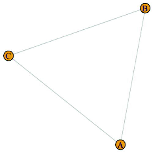
For example, consider a graph G consisting of 3 vertices namely A, B, C which is in the form of a triangle. First, we select an activator, say A. For $i=1$, the vertex A is burnt and at $i=2$ the vertices B and C are burnt. Now we make sure that a vertex is selected as an activator. Thus, at $i=2$, either B or C can be selected as an activator. So, in this example the triangular graph has 2 as its burning number. This is shown in Figure 1.

Figure 1: Example to find the burning number of the graph.

Graph burning problem is being approached by using approximation algorithms and heuristics. These heuristics typically use centrality measures [4] as they have shown to be efficient. Though, centrality measures were efficient it doesn’t attest the problem of randomness. That is whenever there are many nodes with equal centrality the algorithm fails to give an unique burning number. The length of the burning sequence also changes. In this paper, a novel algorithm to find the burning number of a graph is proposed based on selection of activators. The activators were selected based on the core vertex set obtained from spanning tree of the original graph and by using weighted centrality measure. From this list nodes, potential activator is also selected. Using this activators a graph burning algorithm is proposed.

2 Previous work

The initial inspiration for burning of graph came from an idea based on social contagion, how successful an information spreads from a influenced node. Bonato et al. [5] developed the formal definition of burning a graph. A connected graph G is said to be well-burnable if $b(G)\le \lceil \sqrt{n}\rceil$, where n is the order of the graph G. It was proved that any path is well-burnable. Also a graph with a Hamiltonian path is well-burnable. Based on diameter and radius of a graph G, lower bound and upper bound on the burning number were also discussed using the k-distance domination number. Further computation of burning number of a graph G remains to be a NP-complete problem [2]. The approximation algorithm by Bonato and Kamali [6] gives a constant factor of 3 for general graph. The approximation results also implies that the burning problem of a graph is distinct from Firefighter problem. The burning number conjecture is one of the major unsolved problem on burning of graph. Bessy et al. [3] has further refined the upper bound for burning number of a connected graph G.

Farokh et al. [10] has developed six heuristics for the graph burning problem. These algorithms identify the first activator based on center and random vertex selection. The subsequent activators were identified by using far distance and half distance from the previous activator. The dataset used were DIMACS, Benchmarks with Hidden Optimum Solutions for Graph Problems (BHOSLIB), Random $\theta$-graphs and Random graphs with fixed distance to cluster.

Šimon et al. [17] has proposed three heuristics for spreading an alarm throughout a network. The proposed algorithms were Maximum Eigenvector Centrality Heuristic, Cutting Corners Heuristic and Greedy algorithm with Forward-Looking Search Strategy. The maximum eigenvector centrality heuristic looks for the vertices with maximum eigen centrality whereas the cutting corner heuristic looks for the minimum eigen centrality. Both heuristics fails to burn the graph in minimum number of steps. So, an improved greedy algorithm with a forward-looking search strategy incorporated with weighted aggregated sum product assessment was demonstrated with a set consisting 20 central nodes.

Gautam et al. [11] has proposed three heuristics based on centrality. A backbone path of the network graph is found and vertices to be burnt were found using greedy algorithm. The improved cutting corners heuristic works based on the best central nodes. For disconnected graphs, a component based recursive heuristic is also demonstrated by choosing the component with a maximum burning number.

3 The proposed algorithm to obtain the activator

As the burning number problem is NP complete [7], one can obtain a solution for large network graph by a heuristic method. Selection of activators plays a major role in finding the burning number of a graph. In this paper, three different selection methods to select activators are given, followed by a hybrid algorithm to find the burning sequence and the burning number of agraph G.

3.1 Weighted centrality

Centrality measures are used to quantify the importance of a node, and they can be applied to networks and graphs [15]. The word “central” is derived from the Latin word “centrum” which means “place”. Centrality measures are most commonly used in networks to identify which nodes have the most connections, but they can also be applied to graphs with weighted edges or undirected connections. There are many different types of centrality measures, including degree centrality, closeness centrality, eigenvector-based metrics, alpha centrality, beta centrality, etc., [8]. Centrality measures can be used to identify important nodes. For example, if a node with high centrality is deleted, the network will lose some of its functionality.

The most well known is minimum eccentricity of a vertex v where a vertex with the smallest of the maximum graph distance between v and any other node of the network. Degree centrality is simple to use but usually we may encounter same value for two different vertices. The maximum eigenvector centrality has showed more unique values with a few exceptions. If the degree centrality alone is considered, then the problem of randomness peaks up. In order to overcome the problem of randomness we give a higher weight to eigen centrality, $\alpha$ and a least weight to degree centrality, (1-$\alpha$).

The weighted centrality of the vertex v is given by (1) $$w(v)=\alpha e(v)+(1-\alpha )d(v)$$(1) where $e(v)$ is the eigenvector centrality of the vertex v and $d(v)$ is the degree centrality and $\alpha$ lies between 0 and 1. Here, the value of (1-$\alpha$) is obtained from the ratio of total number of vertices with unique value of normalized degree centrality to the total number of vertices for a given network graph G. For a few network graphs the ratio obtained was as low as 0.016. In this case, 0.016 was used as (1-$\alpha$) and 0.984 as $\alpha$.

For example, consider the graph given in Figure 2. Here, the vertices labeled 4, 9, 11 has degree centrality 0.5 and eigen centrality 0.737683, 1, 0.962698, respectively. The weighted centrality is shown in Table 1.

Figure 2: Example to find the potential activator of the graph.

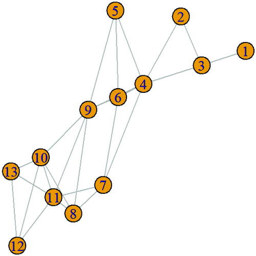
Table 1: Results of weighted centrality.

	Results
Vertex ID	Eigen centrality	Degree	Degree centrality	Weighted centrality
4	0.737683	6	0.5	0.654494
9	1	6	0.5	0.825
11	0.962698	6	0.5	0.800754

3.2 Potential activators

For the selection of the first activator, the weighted centrality is used. However, to find the second activator we may have to consider the fact that we need a shortest burning sequence. We define a vertex set $G^{\prime }$ that is potentially about to receive fire from its previously burned neighbors. So, instead of choosing a larger weighted centrality vertex which is about to receive fire from the previous fired vertex, we may select the next larger weighted centrality vertex. This gives a local optimal solution.

Figure 2, clearly shows that, the vertex 9 is the first activator. From vertex 9, the vertex set {4,5,6,8,10,11} receives fire. For the next level $t=2$, a new activator is to be selected. Here the vertex set {2,3,7,12,13} are about to receive fire from the previously burnt vertex. Thus, at $t=2$, vertex 1 is selected as next activator. For the round $t=3$ the remaining vertices {2,3,7,12,13} are all burnt and one among them is selected as an activator. Hence, the burning sequence of the graph is (9, 1, 13). In this method of selection, even a corner vertex carries information to spread the contagion.

3.3 The spanning tree activator

Spanning trees are used in various fields of computer science. They can be used to build data structures, for routing packets of information, and they are also the backbone of algorithms for computing optimal spanning trees. A spanning tree is a tree that connects all the vertices of a graph with the minimum possible number of edges [12]. It never contains a cycle.

A backbone path is a longest path starting at a node with minimum centrality and containing nodes with high centrality values. A spanning tree itself forms a backbone path. To compute spanning tree, we have used spanning tree function in R studio [9]. By using the spanning tree, a core vertex set is found. That is the vertex with high degree centrality value that occurs in the spanning tree are the best vertex to start burning.

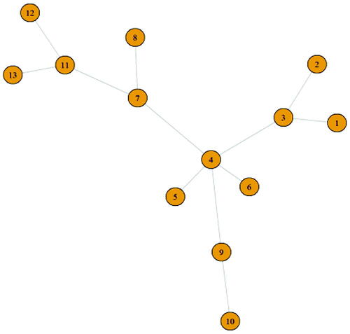
The minimum spanning tree of the graph given in Figure 2 is shown in Figure 3. Here the core vertex set found is 3,4,7,9,11. Instead of checking the whole vertex set the best burning sequence can be found using the core vertex set. In this example, the vertex 4 is selected as the first activator.

Figure 3: Example to find the potential activator of the graph.

3.4 The hybrid algorithm

At the initial stage of the algorithm weighted centrality values of each vertex is computed. The first activator is selected from the core vertex from the spanning tree of graph G. Let v be the vertex with maximum weighted centrality. The neighbor vertex of v was removed that is, all the vertices which are edge connected to v are removed from the graph G. It is labeled as $N_1$. Using $N_1$, we find the neighbor of $N_1$ and labeled as $N_2$. The next potential activators were selected from the vertex that are not an element of $N_1$ and $N_2$. That is, the potential activators were selected from ${(V(G)\cap (N_1\cup N_2))}^{\prime }$. The algorithm ends when all the vertex of the graph G is completely burnt. The process is shown in Algorithm 1.

4 Dataset

The network dataset ca-netscience and ca-sandi-auths [16] is in the category of Collaboration Networks. In this network graph, the vertex represents the author’s name of the researcher and the edges represents the co-authorship. That is two vertices are connected if there is a collaborative work between the two researchers. Thus, the network graph represents the co-authorship of scientists in network theory and experiments. The number of vertices in netscience network graph are 379 and the number of edges in this network graph are 914. The maximum degree of a vertex in this network graph is 34. The other co-authorship network graph is ca-sandi-auths with weights. For simplicity we have removed the weights and used the edge connectivity of the vertices. The number of vertices in this network graph are 86 and the number of edges in this network graph are 124. The maximum degree of a vertex in this network graph is 12. The network graph mahindas [16] is used for economic problem collected by K. Pearson (1983). The number of vertices in this network graph are 1258 and the number of edges are 7682. The maximum degree of a vertex in this network graph is 119. The network graph dolphins [14] is an undirected social network of continual interrelations between 62 dolphins in a neighborhood dwelling off Doubtful Sound, New Zealand. The wide variety of connections between dolphins is 159.

5 Results and discussion

The dataset that was used were ca-netscience and ca-sandi-auths. The results obtained from the proposed method was compared with [5]. Table 2 shows the results of the burning number for hybrid algorithm proposed and that of Bonato’s algorithm. Both big and small datasets were used. It is noted that there is a significant improvement in the proposed hybrid algorithm.

Table 2: Results of burning number.

	Results
Name of the network	Description	|V|	|E|	Max. degree	Bonato	Hybrid Algorithm
netscience	coauthor-ship	379	914	34	12	7
sandi-auths	coauthor-ship	86	124	12	8	6
dolphin	social network	62	159	12	7	5
mahindas	economic problem	1258	7682	119	12	5

In the proposed algorithm, the initial activator is selected based on the core vertex set. This core vertex set is selected based on minimum spanning tree. As a spanning tree never contains cycle, the possibility of a vertex to have high degree due to loop and cycle is ruled out. Thus, the first activator selected based on the core vertex set leads to a best activator. Also, the problem of randomness is avoided using a weighted centrality measure which is based on degree centrality and eigen centrality. Here, higher weight was given to eigen centrality and a lower weight was given to degree centrality. It is also noted that the vertices which were about to receive fire from the previous activators were ignored from being selected as an activator. This enables as to select an activator which doesn’t receives fire which helps to burn the graph faster. This combination of steps makes the algorithm efficient and takes less time while compared to others. As the algorithm searches for vertex at three different layers the time complexity of the proposed algorithm is $O(\log (n^3))$.

6 Conclusion

In this paper, we have proposed an algorithm for finding k-burning number of a graph. The results obtained were compared with Bonato proposed algorithm. We found enhanced results in finding the burning number of the graph. Our algorithm uses spanning tree to find local optimal solution. Using this solution further improvements were made using weighted centrality and also finds potential activators. Future work involves finding the burning number of edges based on edge burning. Also, there are other centrality measures which may help to select the activators. Further, social network graphs are examples of disconnected graph which may need novel graph burning algorithm.

References

- Baron, S., Fons, M., Albrecht, T. (1996). Viral Pathogenesis Medical Microbiology. Galveston, TX: University of Texas. https://www.ncbi.nlm.nih.gov/books/NBK8149/
- Bessy, S., Bonato, A., Janssen, J., Rautenbach, D., Roshanbin, E. (2017). Burning a graph is hard. Discrete Appl. Math. 232: 73–87.
- Bessy, S., Bonato, A., Janssen, J., Rautenbach, D., Roshanbin, E. (2018). Bounds on the burning number. Discrete Appl. Math. 235: 16–22.
- Bloch, F., Jackson, M. O., Tebaldi, P. (2023). Centrality measures in networks. Soc. Choice Welf.
- Bonato, A., Janssen, J., Roshanbin, E. (2016). How to burn a graph. Int. Math. 12(1–2): 85–100.
- Bonato, A., Kamali, S. (2019). Approximation algorithms for graph burning. In: Gopal, T., Watada, J., eds. Theory and Applications of Models of Computation. TAMC 2019. Lecture Notes in Computer Science, 11436. Cham: Springer.
- Bonato, A. (2020). A survey of graph burning. arXiv preprint arXiv:2009.10642.
- Borgatti, S. P. (2005). Centrality and network flow. Soc. Netw. 27(1): 55–71.
- Csardi, G., Nepusz, T. (2006). The igraph software package for complex network research. Int. Complex Syst. 1695(5): 1–9. https://www.researchgate.net/publication/221995787_The_Igraph_Software_Package_for_Complex_Network_Research
- Farokh, Z. R., Tahmasbi, M., Tehrani, Z. H. R. A., Buali, Y. (2020). New heuristics for burning graphs. arXiv preprint arXiv:2003.09314.
- Gautam, R. K., Kare, A. S., Durga Bhavani, S. (2022). Faster heuristics for graph burning. Appl. Intell. 52: 1351–1361.
- Gross, D. J., Saccoman, J. T., Suffel, C. L. (2015). Spanning tree results for graphs and multigraphs: A Matrix-theoretic approach. 10.1142/9789814566049_0002
- Kempe, D., Kleinberg, J., Tardos, É. (2003). Maximizing the spread of influence through a social network. In: Proceedings of the Ninth ACM SIGKDD International Conference on Knowledge Discovery and Data Mining, pp. 137–146.
- Lusseau, D., Schneider, K., Boisseau, O. J., Haase, P., Slooten, E., Dawson, S. M. 2003. The bottlenose dolphin community of Doubtful Sound features a large proportion of long-lasting associations. Behav. Ecol. Sociobiol. 54(4): 396–405.
- Meghanathan, N. (2017). Randomness index for complex network analysis. Soc. Netw. Anal. Min. 7(1): 1–15.
- Rossi, R., Ahmed, N. (2015). The network data repository with interactive graph analytics and visualization. In: Twenty-ninth AAAI Conference on Artificial Intelligence.
- Šimon, M., Huraj, L., Luptáková, I. D., Pospíchal, J. (2019). Heuristics for spreading alarm throughout a network. Appl. Sci. 9(16): 3269.