Two inverse eigenvalue problems for matrices whose graphs are trees

Abstract

Inverse eigenvalue problem refers to the problem of reconstructing a matrix of a desired structure from a prescribed eigendata. In this paper, we discuss two additive inverse eigenvalue problems for matrices whose graph is tree. In order to analyze the problems, the vertices of the given tree are labeled in a suitable way so that concrete recurrence relations between the characteristic polynomials of the leading principal submatrices of the matrix can be obtained in a simple form. The method of obtaining the entries of the required matrix is constructive and provides an algorithm for computing the same. We provide some numerical examples to illustrate the results. The computations are done using SCILAB by feeding the eigendata and the adjacency pattern of the tree as inputs.

KEYWORDS:

• Additive inverse eigenvalue problem
• matrix of a tree
• leading principal submatrices

AMS CLASSIFICATION:

• 05C05
• 65F18

1 Introduction

Inverse eigenvalue problem (IEP) is the problem of reconstructing matrices of pre-assigned structure using the prescribed eigendata. It appears in various applications of mathematics and engineering [3, 11, 12, 21]. One of the ways of describing the structure of the matrix is to represent it by its corresponding graph, where the adjacencies of vertices of the graph correspond to the nonzero off-diagonal entries of the matrix. Inverse problems of constructing matrices described by graphs have been studied by several authors. The off-diagonal entries of such matrices are governed by the adjacency pattern of the vertices in the graph. Graphs are helpful in representing various physical systems in control theory, vibration of string, geophysics, circuit theory, graph theory etc. as can be seen in the papers [3–5] and the eigenvalues of the matrices associated with the graphs govern the behavior of the concerned systems. A detailed characterization of inverse eigenvalue problems has been made by [4]. Inverse eigenvalue problems evolved from the discretization of inverse Strum-Liouville problems and this lead to the study of IEPs of Jacobi matrices [7, 8], Pseudo-Jacobi matrices [22], Periodic Jacobi matrices [23]. IEPs corresponding to different trees have been studied extensively in recent times by several authors. IEPs of constructing matrices using the maximal and minimal eigenvalues of each leading principal submatrices have been solved for bordered diagonal matrices [13, 16], doubly arrow matrices [15]. The problem has been solved for various matrices whose graphs are special trees [1, 2, 6, 17, 19]. A general solution of the extremal IEP for the case of distinct eigenvalues has been given by [20]. [14] studied the reconstruction of a special type of Leslie and doubly Leslie matrices, companion and doubly companion matrices, using maximal eigenvalue of each of the leading principal submatrix and its corresponding eigenvector.

In this paper, we have discussed two additive inverse eigenvalue problems for matrices whose graphs are trees. For a given tree T and a given diagonal matrix D, the first problem is to construct a hollow matrix A corresponding to T, when the largest eigenvalues of each of the leading principal submatrices of the matrix A + D are given. The second problem is to construct a matrix A corresponding to T, when the largest eigenvalues of each of the leading principal submatrices of the matrix A + D are given.

In Section 2, the basic definitions and primary results necessary for solving the above inverse eigenvalue problems have been briefly discussed. Section 4 defines the problems to be discussed in this paper. To solve the problems, the vertices of the trees have been labeled in a suitable manner. Solution of the Problems 1, 2 have been discussed in Sections 3.1 and 3.2, respectively. In Section 4, numerical solutions of the problems are obtained in SCILAB by feeding the eigendata, entries of the diagonal matrices and the adjacency pattern as inputs.

2 Preliminaries

Throughout this paper, the term graph will mean simple undirected graph without any multiple edges and self loops. A graph G consists of a finite set V of elements called vertex set and a set E of unordered pairs of distinct vertices called edge set. The order of the graph G is the number of elements in the vertex set V. Vertices $v_1$ and $v_2$ are adjacent or neighbors, if $e=\{v_1,v_2\}\in E$. A walk in G, joining vertices u and v, is a sequence $\gamma$ of vertices $u=v_0,v_1,\dots ,v_{k-1},v_k=v$ such that $\{v_i,v_{i+1}\}$ is an edge for each $i=0,1,\dots ,k-1$. If the vertices $u=v_0,v_1,\dots ,v_{k-1},v_k=v$ are distinct, then $\gamma$ is called a path joining u and v. If $u=v$ and the vertices $u=v_0,v_1,\dots ,v_{k-1}$ are distinct, then $\gamma$ is a cycle. A graph G is called connected if for each pair of distinct vertices u and v, there is a path joining u and v. A tree is a connected graph without any cycle.

Given an $n\times n$ symmetric matrix $A={(a_{ij})}_{n\times n}$, the graph of A, denoted by $G(A)$, is a graph with vertex set $V=\{1,2,\dots ,n\}$ and edge set $E=\left\{\right\{i,j\}:a_{ij}\ne 0,i\ne j\}$. Since we are considering graphs without any self loops, so the diagonal entries do not have any role to play in describing the adjacency pattern of the graph corresponding to the matrix. For a graph $G=(V,E)$, where $\left|V\right|=n$, $S(G)$ denotes the set of all $n\times n$ symmetric matrices that have G as their graph. Hollow matrix is a matrix whose all diagonal entries are zero. 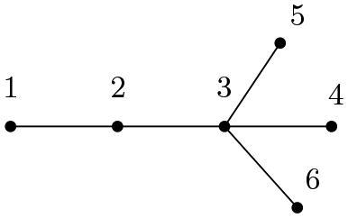The $j\times j$ leading principal submatrix means the $j\times j$ submatrix obtained by retaining the first j rows and j columns of the matrix. Figure 1 shows a special tree named broom with vertex set $V=\{1,2,\dots ,6\}$ and its corresponding matrix.

Figure 1: A broom and its matrix.

The expression for the determinant ([9]) of a matrix A is given by, (1) $$\det A=\sum _{\sigma }\left(\text{sgn}\sigma \prod _{i=1}^n{a}_{i\sigma (i)}\right)$$(1) where the summation runs over all the n! permutations of $\{1,2,\dots ,n\}$ and $\text{sgn}\sigma$, the sign of permutation $\sigma$, is $+1$ if the permutation $\sigma$ is even or $-1$ if $\sigma$ is odd.

Lemma 2.1.

For a tree, the determinant of the corresponding matrix A is given by (2) $$\det A=\sum _{\sigma }\left(\text{sgn}\sigma \prod _{i=1}^n{a}_{i\sigma (i)}\right)$$(2) where the summation runs over all those permutations of $\{1,2,\dots ,n\}$ which are either a transposition or a product of disjoint transpositions in the cycle decomposition of $\sigma$.

Proof.

For any square matrix A, its determinant is given by equation (1)(1) $$\det A=\sum _{\sigma }\left(\text{sgn}\sigma \prod _{i=1}^n{a}_{i\sigma (i)}\right)$$(1) . We claim that the product ${\prod }_{i=1}^n{a}_{i\sigma (i)}=0$ whenever $\sigma$ has a cycle of length more than 2. Let some permutation $\sigma$ in the summation 1 contains a cycle $(i_1,i_2,\dots ,i_r)$ of length $r>2$. Now, if the product term corresponding to this permutation is non-zero, then $a_{i_k\sigma (i_k)}\ne 0$ for all k. Thus the vertices $v_{i_1},v_{i_2},\dots ,v_{i_r}$ form a cycle in the tree, a contradiction. Hence, the summation runs over all those permutations of $\{1,2,\dots ,n\}$ which are either a transposition or a product of disjoint transpositions only in the cycle decomposition of $\sigma$. ▪

Further, given any $i\in V=\{1,2,\dots ,n\}$, there are two possibilities for any permutation $\sigma$ of V, either $\sigma (i)=i$ or $\sigma (i)\ne i$. Thus, the summation in equation (2)(2) $$\det A=\sum _{\sigma }\left(\text{sgn}\sigma \prod _{i=1}^n{a}_{i\sigma (i)}\right)$$(2) can be split as (3) $$\begin{array}{cc}\det A=\hfill & \sum _{\sigma (i)=i}\left(\text{sgn}\sigma \prod _{i=1}^n{a}_{i\sigma (i)}\right)+\sum _{\sigma (i)\ne i}\left(\text{sgn}\sigma \prod _{i=1}^n{a}_{i\sigma (i)}\right)\hfill \end{array}$$(3)

For permutations $\sigma$ with $\sigma (i)=i$, the sign of $\sigma$ restricted to $V\setminus \left\{i\right\}$ is same as that of $\sigma$. For $\sigma (i)\ne i$, $a_{i\sigma (i)}\ne 0$ if and only if $\sigma (i)\sim i$, that is $\sigma (i)$ is adjacent to i. Thus, we can extract $a_{ii}$ from all the terms in the first summation of equation (3)(3) $$\begin{array}{cc}\det A=\hfill & \sum _{\sigma (i)=i}\left(\text{sgn}\sigma \prod _{i=1}^n{a}_{i\sigma (i)}\right)+\sum _{\sigma (i)\ne i}\left(\text{sgn}\sigma \prod _{i=1}^n{a}_{i\sigma (i)}\right)\hfill \end{array}$$(3) . We can also extract $a_{ij}{a}_{ji}$ for each $j\sim i$ in the second summation. Let $A(i)$ denote the principal submatrix obtained from A by deleting its ith row and column and $A(i,j)$ is the principal submatrix obtained from A by deleting its i-th and j-th rows and columns. Thus, the expression for the determinant of a matrix whose graph is a tree can be reduced to (4) $$\begin{array}{cc}\det A=\hfill & a_{ii}\det A(i)-\sum _{j\sim i}{a}_{ij}^2\det A(i,j)\hfill \end{array}$$(4)

In this paper, we will solve the following two problems:

Problem 1.

Given a tree on n vertices and an $n\times n$ diagonal matrix D and n real numbers ${\lambda }_1,{\lambda }_2,\dots ,{\lambda }_n$, find a hollow matrix $A\in S(T)$ such that each ${\lambda }_j$ is the largest eigenvalue of the $j\times j$ leading principal submatrix of $A+D$.

Problem 2.

Given a tree on n vertices and an $n\times n$ diagonal matrix D and n real numbers ${\lambda }_1,{\lambda }_2,\dots ,{\lambda }_n$, find a matrix $A\in S(T)$ such that each ${\lambda }_j$ is the largest eigenvalue of the $j\times j$ leading principal submatrix of $A+D$.

3 Solution to the IEPs

We adopt a standard way of labeling the vertices of the tree in a suitable manner which provides a simplified recurrence relation between the characteristic polynomials of each leading principal submatrix. This scheme of labeling was referred to as successively connected labeling by [20]. For a given tree T, it is always possible to label the vertices of the tree in such a way that each vertex j remains adjacent to exactly one of the vertices from the set $\{1,2,\dots ,j-1\}$. The scheme of labeling is given below :

1. We choose any vertex of T and label it as 1.

2. Then we choose any unlabeled vertex which is adjacent to 1 and label it as 2.

3. Proceeding this way, at the jth step, we label as j any unlabeled vertex which is adjacent to one of the already labeled vertices.

4. We continue this process till all the vertices of T are labeled from 1 to n.

In the above scheme of labeling, the induced subgraph $T_j$ corresponding to the vertices $\{1,2,\dots ,j\}$ is a tree for each $j=1,2,\dots ,n$. Also, each vertex j is adjacent to exactly one of the vertices of $\{1,2,\dots ,j-1\}$. Let $v(j)$ denote the unique vertex among $\{1,2,\dots ,j-1\}$ that is adjacent to j. An example of successively connected labeling of a tree is illustrated in the following Figure 2:

Figure 2: Successively connected labelling.

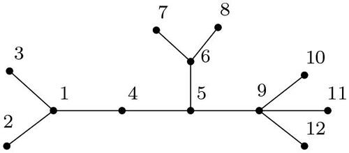
Here, $v(2)=v(3)=v(4)=1$, $v(5)=4$, $v(6)=5$, $\dots$, $v(11)=9$.

Following Lemmas will be useful in solving the IEPs:

Lemma 3.1.

[20] Let $P(\lambda )$ be a monic polynomial of degree n with all real zeros and ${\lambda }_{\min }$ and ${\lambda }_{\max }$ be the minimal and maximal zeros of P, then

1. If $\mu <{\lambda }_{\min }$, then ${(-1)}^{n}P(\mu )>0$.

2. If $\mu >{\lambda }_{\max }$, then $P(\mu )>0$.

Lemma 3.2.

[10] If T is a tree, the largest and smallest eigenvalues of each matrix A in $S(T)$, have multiplicity 1. Moreover, the largest or smallest eigenvalue of a matrix A in $S(T)$ cannot occur as an eigenvalue of a submatrix $A(v)$, for any vertex v of T .

Theorem 3.3.

(Cauchy’s Interlacing Theorem) [9] Let ${\lambda }_1\le {\lambda }_2\le \dots \le {\lambda }_n$ be the eigenvalues of any $n\times n$ real symmetric matrix A and ${\mu }_1\le {\mu }_2\le \dots \le {\mu }_{n-1}$ be the eigenvalues of any of its submatrix of order $(n-1)\times (n-1)$ then $${\lambda }_1\le {\mu }_1\le {\lambda }_2\le {\mu }_2\le \dots \le {\lambda }_{n-1}\le {\mu }_{n-1}\le {\lambda }_n$$

By Cauchy’s Interlacing Theorem 3.3, the largest eigenvalue of any matrix is greater than or equal to the eigenvalues of its submatrices. As an immediate consequence, we have the following necessary condition for the solution of the problems of section 4

Lemma 3.4.

A necessary condition for the existence of solutions to the problems 1 and 2 is ${\lambda }_1\le {\lambda }_2\le \dots \le {\lambda }_n$.

Lemma 3.5.

Let A be a matrix in $S(T)$ corresponding to a given successively connected labeling of T. Then the largest eigenvalues of the leading principal submatrices of A are distinct from each other.

Proof.

Since the tree has successively connected labeling, the induced submatrix corresponding to the vertices $\{1,2,\dots ,j\}$ is a tree for each $j=1,2,\dots ,n$. Thus, $T_j$ is a tree for each j. Then, by Lemma 3.2, the largest eigenvalue of $T_j$ cannot occur as the largest eigenvalue of $T_{j-1}$. Hence, the largest eigenvalues of each leading principal submatrix of the corresponding matrix of T are distinct. ▪

3.1 Solution to the problem 1

Let T denote a tree with successively connected labeling. A be any hollow matrix whose corresponding graph is T and $D=\mathit{diag}(d_1,d_2,\dots ,d_n)$ be the given diagonal matrix. The entries of A are to be computed.

Lemma 3.6.

Let $X=A+D$ and $X_j$ be the $j\times j$ leading principal submatrix of X. The sequence $P_j(\lambda )=\det (\lambda I_j-X_j)$ satisfies the following recurrence relation:

1. $P_1(\lambda )=\lambda -d_1$

2. $P_j(\lambda )=(\lambda -d_j)P_{j-1}(\lambda )-a_{jv(j)}^2{Q}_j(\lambda )\mathit{forj}=2,3,\dots ,n$

where $Q_j(\lambda )$ is the characteristic polynomial of the principal submatrix of $X_j$ obtained by deleting the rows and columns indexed by j and $v(j)$, $D=\mathit{diag}(d_1,d_2,\dots ,d_n)$ and for convenience of notation, we take $Q_2(\lambda )=1$.

Proof.

The expression for $P_j(\lambda )$ can be obtained by expanding the determinant of $\lambda I_j-X_j$ using equation (4)(4) $$\begin{array}{cc}\det A=\hfill & a_{ii}\det A(i)-\sum _{j\sim i}{a}_{ij}^2\det A(i,j)\hfill \end{array}$$(4) . ▪

Theorem 3.7.

For distinct ${\lambda }_i$‘s, Problem 1 has a solution iff

1. ${\lambda }_1=d_1$.

2. ${\lambda }_j>d_j$, for $j=2,3,\dots ,n$.

Proof.

Since ${\lambda }_j$ is a zero of $P_j$ for each j, so $P_1({\lambda }_1)=0\Rightarrow {\lambda }_1=d_1$. Also, $$\begin{array}{c}{P}_j({\lambda }_j)=0\\ \Rightarrow a_{jv(j)}^2=\frac{({\lambda }_j-d_j)P_{j-1}({\lambda }_j)}{Q_j({\lambda }_j)}\end{array}$$

Here, $Q_j({\lambda }_j)\ne 0$ follows from Cauchy’s interlacing theorem and the fact that each ${\lambda }_j$ is the largest eigenvalue of $X_j$. By Lemma 3.1, $P_{j-1}({\lambda }_j)>0$ and $Q_j({\lambda }_j)>0$. Thus, $a_{jv(j)}^2>0$ if and only if ${\lambda }_j-d_j>0$ i.e. ${\lambda }_j>d_j$. ▪

The above results leads to Algorithm 3.1 which can be compiled into a SCILAB code to get the solutions:

Algorithm 3.1

1. Input an $n\times n$ diagonal matrix D, eigendata ${\lambda }_1<{\lambda }_2<\dots <{\lambda }_n$.

2. Label the vertices of T following successively connected labeling and input the adjacency pattern of the corresponding matrix A.

3. If ${\lambda }_1=d_1$ and ${\lambda }_j>d_j$, for $j=2,3,\dots ,n$ Then $$a_{jv(j)}^2=\frac{({\lambda }_j-d_j)P_{j-1}({\lambda }_j)}{Q_j({\lambda }_j)}$$

Else No solution

EndIf

3.2 Solution to the problem 2

Let T denote a tree with successively connected labeling. Let A be any matrix whose corresponding graph is T and $D=\mathit{diag}(d_1,d_2,\dots ,d_n)$ be the given diagonal matrix.

Lemma 3.8.

Let $X=A+D$ and $X_j$ be the $j\times j$ leading principal submatrix of X. The sequence $P_j(\lambda )=\det (\lambda I_j-X_j)$ satisfies the following recurrence relation:

1. $P_1(\lambda )=\lambda -d_1-a_{11}$

2. $P_j(\lambda )=(\lambda -d_j-a_{jj})P_{j-1}(\lambda )-a_{jv(j)}^2{Q}_j(\lambda )\mathit{forr}=2,3,\dots ,n$

where $Q_j(\lambda )$ is the characteristic polynomial of the principal submatrix of $X_j$ obtained by deleting the rows and columns indexed by j and $v(j)$, $D=\mathit{diag}(d_1,d_2,\dots ,d_n)$.

Proof.

The expression for $P_j(\lambda )$ can be obtained by expanding the determinant of $\lambda I_j-X_j$ using equation (4)(4) $$\begin{array}{cc}\det A=\hfill & a_{ii}\det A(i)-\sum _{j\sim i}{a}_{ij}^2\det A(i,j)\hfill \end{array}$$(4) . ▪

Theorem 3.9.

Suppose all ${\lambda }_i$‘s are distinct, then the Problem 2 has infinite numbers of solutions.

Proof.

Since ${\lambda }_r$ is a zero of $P_r$ for each r, $P_1({\lambda }_1)=0\Rightarrow a_{11}={\lambda }_1-d_1$. $$\begin{array}{c}{P}_j({\lambda }_j)=0\\ \Rightarrow a_{jv(j)}^2=\frac{({\lambda }_j-a_{jj}-d_j)P_{j-1}({\lambda }_j)}{Q_j({\lambda }_j)}\end{array}$$

Here, $Q_j({\lambda }_j)\ne 0$ follows from Cauchy’s interlacing theorem and the fact that each ${\lambda }_j$ is the largest eigenvalue of $X_j$. By Lemma 3.1, $P_{j-1}({\lambda }_j)>0$ and $Q_j({\lambda }_j)>0$. Thus, $a_{jv(j)}^2>0$ if and only if ${\lambda }_j-a_{jj}-d_j>0$ i.e. ${\lambda }_j>a_{jj}+d_j$. In order to obtain a solution, we choose $a_{jj}$ such that $a_{jj}<{\lambda }_j-d_j$. For each $a_{jj}<{\lambda }_j-d_j$ we get a value of $a_{jv(j)}^2$. So, the above problem has infinitely many solutions. ▪

The above results leads to Algorithm 3.2 which can be compiled into a SCILAB code to get the solutions :

Algorithm 3.2

1. Input an $n\times n$ diagonal matrix D, eigendata ${\lambda }_1<{\lambda }_2<\dots <{\lambda }_n$.

2. Label the vertices of T following successively connected labeling and input the adjacency pattern of the corresponding matrix A.

3. Set $a_{11}={\lambda }_1-d_1$.

4. For $j=2,\dots ,n$

5. Choose $a_{jj}$ such that $a_{jj}<{\lambda }_j-d_j$

6. Use $a_{jj}$ to compute $a_{jv(j)}^2=\frac{({\lambda }_j-a_{jj}-d_j)P_{j-1}({\lambda }_j)}{Q_j({\lambda }_j)}$

EndFor

Solution of the above two problems depends on how the vertices of the trees have been labeled. We will show it with an example that two different labeling will give rise to two different solutions.

4 Numerical examples

Numerical solutions to some particular problems has been obtained here using SCILAB programming.

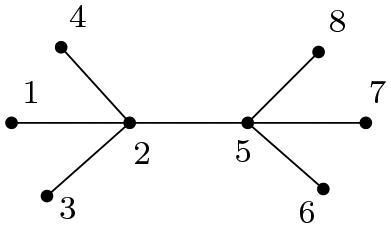
Example 4.1.

Given a tree T on 8 vertices as shown in the figure below, 8 real numbers ${\lambda }_1=1,{\lambda }_2=3,{\lambda }_3=4,{\lambda }_4=5,{\lambda }_5=6,{\lambda }_6=7,{\lambda }_7=8,{\lambda }_8=9$ and the diagonal matrix is $D=\mathit{diag}(1,2,3,4,5,6,7,8)$, find a hollow matrix $A\in S(T)$ such that ${\lambda }_j$ is the largest eigenvalue of the $j\times j$ leading principal submatrix of $A+D$ for each j.

Solution 1.

The vertices of the tree have been labeled in two ways following the scheme of successively connected labeling. For the first way of labeling (Figure 3), $v(2)=1,v(3)=v(4)=v(5)=2,v(6)=v(7)=v(8)=5$. The required matrix obtained using SCILAB is $$\left(\mathrm{}\mathrm{}\begin{array}{cccccccc}\mathit{cccccccc}0& 1.4142136& 0& 0& 0& 0& 0& 0\\ 1.4142136& 0& 1.1547005& 1.3540064& 1.4962917& 0& 0& 0\\ 0& 1.1547005& 0& 0& 0& 0& 0& 0\\ 0& 1.3540064& 0& 0& 0& 0& 0& 0\\ 0& 1.4962917& 0& 0& 0& 1.1825851& 1.3608846& 1.4981445\\ 0& 0& 0& 0& 1.1825851& 0& 0& 0\\ 0& 0& 0& 0& 1.3608846& 0& 0& 0\\ 0& 0& 0& 0& 1.4981445& 0& 0& 0\end{array}\mathrm{}\mathrm{}\right)$$

Figure 3: Refer Example 4.1 (First way).

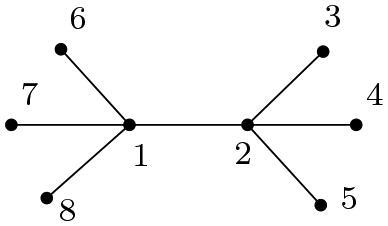
For the second way of labeling (Figure 4), $v(2)=v(6)=v(7)=v(8)=1=1,v(3)=v(4)=v(5)=2$. The required matrix obtained using SCILAB is $$\left(\begin{array}{cccccccc}0& 1.4142136& 0& 0& 0& 2.3062582& 1.9745782& 1.9838798\\ 1.4142136& 0& 1.1547005& 1.3540064& 1.4962917& 0& 0& 0\\ 0& 1.1547005& 0& 0& 0& 0& 0& 0\\ 0& 1.3540064& 0& 0& 0& 0& 0& 0\\ 0& 1.4962917& 0& 0& 0& 0& 0& 0\\ 2.3062582& 0& 0& 0& 0& 0& 0& 0\\ 1.9745782& 0& 0& 0& 0& 0& 0& 0\\ 1.9838798& 0& 0& 0& 0& 0& 0& 0\end{array}\right)$$

Figure 4: Refer Example 4.1 (Second way).

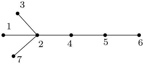
Example 4.2.

Given the broom T (Figure 5) on 7 vertices, 7 real numbers ${\lambda }_1=3,{\lambda }_2=5,{\lambda }_3=9,{\lambda }_4=10,{\lambda }_5=13,{\lambda }_6=18,{\lambda }_7=20$ and the diagonal matrix $D=\mathit{diag}(1,4,7,9,11,13,17)$, find $A\in S(T)$ such that ${\lambda }_j$ is the largest eigenvalue of the $j\times j$ leading principal submatrix of $A+D$ for each j.

Figure 5: Refer Example 4.2.

Solution 2.

There are infinitely many solutions of this problem. Here, we show two solutions obtained using SCILAB. As per the labeling, $v(2)=1,v(3)=v(4)=v(7)=2,v(5)=4,v(6)=5$. The solution obtained by taking $a_{22}=a_{33}=0,a_{44}=-1,a_{55}=1,a_{66}=3$ and $a_{77}=1$ is $$A=\left(\begin{array}{ccccccc}2& 1.4142136& 0& 0& 0& 0& 0\\ 1.4142136& 0& 1.8973666& 3.0047581& 0& 0& 5.4411388\\ 0& 1.8973666& 0& 0& 0& 0& 0\\ 0& 3.0047581& 0& -1& 1.9745771& 0& 0\\ 0& 0& 0& 1.9745771& 1& 3.3413312& 0\\ 0& 0& 0& 0& 3.3413312& 3& 0\\ 0& 5.4411388& 0& 0& 0& 0& 1\end{array}\right)$$

The solution obtained by taking $a_{22}=-1,a_{33}=a_{44}=a_{55}=0,a_{66}=4$ and $a_{77}=2$ is the following matrix $$A=\mathrm{}\left(\begin{array}{ccccccc}2& 2& 0& 0& 0& 0& 0\\ 2& -1& 3.2659863& 1.6949973& 0& 0& 3.9567092\\ 0& 3.2659863& 0& 0& 0& 0& 0\\ 0& 1.6949973& 0& 0& 2.6954447& 0& 0\\ 0& 0& 0& 2.6954447& 0& 2.4846656& 0\\ 0& 0& 0& 0& 2.4846656& 4& 0\\ 0& 3.9567092& 0& 0& 0& 0& 2\end{array}\right)$$

5 Conclusion

In this paper, we have provide the sufficient condition for the construction of matrix whose corresponding graph is a tree under a specific scheme of labeling. We have dealt with the case where the given eigenvalues are distinct. the case for non-distinct eigenvalues can be studied further. The problem can also be studied for different connected graphs like unicyclic, multicyclic graphs and also with other types of labelings.

References

- Babaei Zarch, M., Fazeli, S. A. S., Karbassi, S. M. (2018). Inverse eigenvalue problem for matrices whose graph is a banana tree. J. Algorithms Comput. 50(2): 89–101.
- Babaei Zarch, M., Fazeli, S. A. S. (2019). Inverse eigenvalue problem for a kind of acyclic matrices. Iran. J. Sci. Technol. Trans. A: Sci. 43: 2531–2539.
- Barcilon, V. (1976). On the solution of the inverse problem with amplitude and natural frequency data, Part I. Phys. Earth Planet. Inter. 13(1): P1–P8.
- Chu, M. T. (1998). Inverse eigenvalue problems. SIAM Rev. 40(1): 1–39.
- Gladwell, G. M. L. (1998). Inverse problems in vibration. Appl. Mech. Rev. 39(7): 1013–1018.
- Heydari, M., Fazeli, S. A. S., Karbassi, S. M. (2019). On the inverse eigenvalue problem for a special kind of acyclic matrices. Appl. Math. 64: 351–366.
- Hochstadt, H. (1967). On some inverse problems in matrix theory. Archiv der Math. 18: 201–207.
- Hochstadt, H. (1974). On the construction of a Jacobi matrix from spectral data. Linear Algebra Appl. 8: 435–446.
- Horn, R. A., Johnson, C. R. (2012). Matrix Analysis, 2nd ed. Cambridge: Cambridge University Press.
- Johnson, C. R., Duarte, A. L., Saiago, C. M. (2003). Inverse eigenvalue problems and lists of multiplicities of eigenvalues for matrices whose graph is a tree: the case of generalized stars and double generalized stars. Linear Algebra Appl. 373: 311–330.
- Li, N. (1997). A matrix inverse eigenvalue problem and its application. Linear Algebra Appl. 266: 143–152.
- Nylen, P., Uhlig, F. (1997). Inverse eigenvalue problems associated with spring-mass systems. Linear Algebra Appl. 254(1): 409–425. Proceeding of the Fifth Conference of the International Linear Algebra Society.
- Peng, J., Hu, X.-Y., Zhang, L. (2006). Two inverse eigenvalue problems for a special kind of matrices. Linear Algebra Appl. 416(2): 336–347.
- Pickmann-Soto, H., Arela-Prez, S., Nina, H., Valero, E. (2020). Inverse maximal eigenvalues problems for Leslie and doubly Leslie matrices. Linear Algebra Appl. 592: 93–112.
- Pickmann, H., Egaña, J., Soto, R. (2009). Two inverse eigenproblems for symmetric doubly arrow matrices. Electron. J. Linear Algebra 18: 700–718.
- Pickmann, H., Egaa, J., Soto, R. L. (2007). Extremal inverse eigenvalue problem for bordered diagonal matrices. Linear Algebra Appl. 427(2): 256–271.
- Sharma, D., Sen, M. (2016). Inverse eigenvalue problems for two special acyclic matrices. Mathematics 4(1): 12.
- Sharma, D., Sen, M. (2018). Inverse eigenvalue problems for acyclic matrices whose graph is a dense centipede. Spec. Matrices 6(1): 77–92.
- Sharma, D., Sen, M. (2021). The minimax inverse eigenvalue problem for matrices whose graph is a generalized star of depth 2. Linear Algebra Appl. 621: 334–344.
- Sharma, D., Kumar Sarma, B. (2022). Extremal inverse eigenvalue problem for irreducible acyclic matrices. Appl. Math. Sci. Eng. 30(1): 192–209.
- Wei, Y., Dai, H. (2016). An inverse eigenvalue problem for the finite element model of a vibrating rod. J. Comput. Appl. Math. 300: 172–182.
- Xu, W.-R., Bebiano, N., Chen, G.-L. (2019). An inverse eigenvalue problem for pseudo-Jacobi matrices. Appl. Math. Comput. 346: 423–435.
- Xu, Y.-H., Jiang, E.-X. (2006). An inverse eigenvalue problem for periodic Jacobi matrices. Inverse Problems 23(1): 165–181.