Squared distance matrices of trees with matrix weights

Abstract

Let T be a tree on n vertices whose edge weights are positive definite matrices of order s. The squared distance matrix of T, denoted by Δ, is the ns × ns block matrix with ${\Delta }_{ij}=d{(i,j)}^2$, where d(i, j) is the sum of the weights of the edges in the unique (i, j)-path. In this article, we obtain a formula for the determinant of Δ and find ${\Delta }^{-1}$ under some conditions.

KEYWORDS:

• Tree
• distance matrix
• squared distance matrix
• matrix weight
• determinant
• inverse

AMS CLASSIFICATION:

• 05C22
• 05C50

1 Introduction

Let T be a tree with vertex set $V(T)=\{1,\dots ,n\}$ and edge set $E(T)=\{e_1,\dots ,e_{n-1}\}$. If two vertices i and j are adjacent, we write $i\sim j$. Let us assign an orientation to each edge of T. The usual distance between the vertices $i,j\in V(T)$, denoted by $d_u(i,j)$, is the length of the shortest path between them in T. Two edges $e_i=(p,q)$ and $e_j=(r,s)$ of T are similarly oriented if $d_u(p,r)=d_u(q,s)$ and is denoted by $e_i\Rightarrow e_j$, otherwise they are oppositely oriented and is denoted by $e_i\rightleftharpoons e_j$. The edge orientation matrix $H=(h_{ij})$ of T is the $(n-1)\times (n-1)$ matrix whose rows and columns are indexed by the edges of T and the entries are defined [8] as $$h_{ij}=\{\begin{array}{cc}1\hfill & \hspace{1em}\text{if }{e}_i\Rightarrow e_j,i\ne j;\hfill \\ -1\hfill & \hspace{1em}\text{if }{e}_i\rightleftharpoons e_j,i\ne j;\hfill \\ 1\hfill & \hspace{1em}\text{if }i=j.\hfill \end{array}$$

The incidence matrix Q of T is the $n\times n-1$ matrix with its rows indexed by V(T) and the columns indexed by E(T). The entry corresponding to the row i and column e_j of Q is 1 if e_j originates at i,–1 if e_j terminates at i, and zero if e_j and i are not incident. We assume that the same orientation is used while defining the edge orientation matrix H and the incidence matrix Q.

The distance matrix of T, denoted by D(T), is the $n\times n$ matrix whose rows and columns are indexed by the vertices of T and the entries are defined as follows: $D(T)=(d_{ij})$, where $d_{ij}=d_u(i,j)$. In [8], the authors introduced the notion of squared distance matrix Δ, which is defined to be the Hadamard product $D°D$, that is, the (i, j)-th element of Δ is $d_{ij}^2$. For the unweighted tree T, the determinant of Δ is obtained in [8], while the inverse and the inertia of Δ are considered in [7]. In [5], the author considered an extension of these results to a weighted tree whose each edge is assigned a positive scalar weight and found the determinant and inverse of Δ. Recently, in [9], the authors determined the inertia and energy of the squared distance matrix of a complete multipartite graph. Also, they characterized the graphs among all complete t-partite graphs on n vertices for which the spectral radius of the squared distance matrix and the squared distance energy are maximum and minimum, respectively.

In this article, we consider a weighted tree T on n vertices with each edge weight is a positive definite matrix of order s. For $i,j\in V(T)$, the distance d(i, j) between i and j is the sum of the weight matrices in the unique (i, j)-path of T. Thus, the distance matrix $D=(d_{ij})$ of T is the block matrix of order ns × ns with its (i, j)-th block $d_{ij}=d(i,j)$ if $i\ne j$, and is the s × s zero matrix if i = j. The squared distance matrix Δ of T is the ns × ns block matrix with its (i, j)-th block is equal to $d{(i,j)}^2$ if $i\ne j$, and is the s × s zero matrix if i = j. The Laplacian matrix $L=(l_{ij})$ of T is the ns × ns block matrix defined as follows: For $i,j\in V(T),i\ne j$, the (i, j)-th block $l_{ij}=-{(W(i,j))}^{-1}$ if i ~ j, where W(i, j) is the matrix weight of the edge joining the vertices i and j, and the zero matrix otherwise. For $i\in V(T)$, the (i, i)-th block of L is $\sum _{j\sim i}(W(i,j){)}^{-1}$.

In the context of classical distance, the matrix weights have been studied in [2] and [3]. The Laplacian matrix with matrix weights have been studied in [2, 10] and [11]. The Resistance distance matrix and the Product distance matrix with matrix weights have been considered in [1], and [6], respectively. In this article, we consider the squared distance matrix Δ of a tree T with matrix weights and find the formulae for the determinant and inverse of Δ, which generalizes the results of [5, 7, 8].

This article is organized as follows. In Section 2, we define needed notations and state some preliminary results, which will be used in the subsequent sections. In Section 3, we find some relations of incidence matrix, Laplacian matrix, and distance matrix with squared distance matrix. In Sections 4 and 5, we obtain the formula for the determinant and inverse of Δ, respectively.

2 Notations and preliminary results

In this section, we define some useful notations and state some known results which will be needed to prove our main results.

The $n\times 1$ column vector with all ones and the identity matrix of order n are denoted by ${\mathbf{1}}_n$ and I_n, respectively. Let J denote the matrix of appropriate size with all entries equal to 1. The transpose of a matrix A is denoted by $A^{\prime }$. Let A be an n × n matrix partitioned as $A=\left[\begin{array}{cc}{A}_{11}& A_{12}\\ A_{21}& A_{22}\end{array}\right]$, where A₁₁ and A₂₂ are square matrices. If A₁₁ is nonsingular, then the Schur complement of A₁₁ in A is defined as $A_{22}-A_{21}{A}_{11}^{-1}{A}_{12}$. The following is the well known Schur complement formula: $\det A=(\det A_{11})\det (A_{22}-A_{21}{A}_{11}^{-1}{A}_{12})$. The Kronecker product of two matrices $A={(a_{ij})}_{m\times n}$ and $B={(b_{ij})}_{p\times q}$, denoted by $A\otimes B$, is defined to be the mp × nq block matrix $[a_{ij}B]$. It is known that for the matrices A, B, C and D, $(A\otimes B)(C\otimes D)=AC\otimes BD$, whenever the products AC and BD are defined. Also ${(A\otimes B)}^{-1}=A^{-1}\otimes B^{-1}$, if A and B are nonsingular. Moreover, if A and B are n × n and p × p matrices, respectively, then $\det (A\otimes B)={(\det A)}^p{(\det B)}^n$. For more details about the Kronecker product, we refer to [12].

Let H be the edge-orientation matrix, and Q be the incidence matrix of the underlying unweighted tree with an orientation assigned to each edge. The edge-orientation matrix of a weighted tree whose edge weights are positive definite matrices of order s is defined by replacing 1 and–1 by I_s and $-I_s$, respectively. The incidence matrix of a weighted tree is defined in a similar way. That is, for the matrix weighted tree T, the edge-orientation matrix and the incidence matrix are defined as $(H\otimes I_s)$ and $(Q\otimes I_s)$, respectively. For a block matrix A, let A_ij denote the (i, j)-th block of A.

Now we introduce some more notations. Let T be a tree with vertex set $V(T)=\{1,\dots ,n\}$ and edge set $E(T)=\{e_1,\dots ,e_{n-1}\}$. Let W_i be the edge weight matrix associated with each edge e_i of T, $i=1,2,\dots ,n$. Let δ_i be the degree of the vertex i and set ${\tau }_i=2-{\delta }_i$ for $i=1,2,\dots ,n$. Let τ be the $n\times 1$ matrix with components ${\tau }_1,\dots ,{\tau }_n$ and $\tilde{\tau }$ be the diagonal matrix with diagonal entries ${\tau }_1,{\tau }_2,\dots ,{\tau }_n$. Let $\widehat{{\delta }_i}$ be the matrix weighted degree of i, which is defined as $$\widehat{{\delta }_i}=\sum _{j:j\sim i}W(i,j), i=1,\dots ,n.$$

Let $\widehat{\delta }$ be the ns × s block matrix with the components $\widehat{{\delta }_1},\dots ,\widehat{{\delta }_n}$. Let F be a diagonal matrix with diagonal entries $W_1,W_2,\dots ,W_{n-1}$. It can be verified that $L=(Q\otimes I_s)F^{-1}$ $(Q^{\prime }\otimes I_s)$.

A tree T is said to be directed tree, if the edges of the tree T are directed. If the tree T has no vertex of degree 2, then $\widehat{\tau }$ denote the diagonal matrix with diagonal elements $1/{\tau }_1,1/{\tau }_2,\dots ,1/{\tau }_n$. In the following theorem, we state a basic result about the edge-orientation matrix H of an unweighted tree T, which is a combination of Theorem 9 of [8] and Theorem 11 of [7].

Theorem 2.1.

[7, 8] Let T be a directed tree on n vertices and let H and Q be the edge-orientation matrix and incidence matrix of T, respectively. Then $\det H=2^{n-2}{\prod }_{i=1}^n{\tau }_i$. Furthermore, if T has no vertex of degree 2, then H is nonsingular and $H^{-1}=\frac{1}{2}{Q}^{\prime }\widehat{\tau }Q$.

Next, we state a known result related to the distance matrix of a tree with matrix weights.

Theorem 2.2.

[2, Theorem 3.4] Let T be a tree on n vertices whose each edge is assigned a positive definite matrix of order s. Let L and D be the Laplacian matrix and distance matrix of T, respectively. If D is invertible, then the following assertions hold:

1. $LD=\tau {\mathbf{1}}_n^{\prime }\otimes I_s-2I_n\otimes I_s$.

2. $DL={\mathbf{1}}_n{\tau }^{\prime }\otimes I_s-2I_n\otimes I_s.$

3 Properties of the squared distance matrices of trees

In this section, we find the relation of the squared distance matrix with other matrices, such as distance matrix, Laplacian matrix, incidence matrix, etc. We will use these results to obtain the formulae for determinants and inverses of the squared distance matrices of directed trees.

Lemma 3.1.

Let T be a tree with vertex set $\{1,2,\dots ,n\}$ and each edge of T is assigned a positive definite matrix weight of order s. Let D and Δ be the distance matrix and the squared distance matrix of T, respectively. Then $\Delta (\tau \otimes I_s)=D\widehat{\delta }.$

Proof.

Let $i\in \{1,2,\dots ,n\}$ be fixed. For $j\ne i$, let p(j) be the predecessor of j on the (i, j)-path of the underlying tree. Let e_j be the edge between the vertices p(j) and j. Let W_j be the weight of the edge e_j and $X_j=\widehat{{\delta }_j}-W_j$. Therefore, $$\begin{array}{c}2\sum _{j=1}^{n}d{(i,j)}^2=\sum _{j=1}^{n}d{(i,j)}^2+\sum _{j\ne i}(d(i,p(j))+W_j{)}^2\\ =\sum _{j=1}^{n}d{(i,j)}^2+\sum _{j\ne i}d{(i,p(j))}^2\\ + 2\sum _{j\ne i}d(i,p(j))W_j+\sum _{j\ne i}{W}_j^2.\end{array}$$

Since the vertex j is the predecessor of ${\delta }_j-1$ vertices in the paths from i, we have $$\sum _{j\ne i}d{(i,p(j))}^2=\sum _{j=1}^n({\delta }_j-1)d{(i,j)}^2.$$

Thus, $$\begin{array}{c}2\sum _{j=1}^{n}d{(i,j)}^2=\sum _{j=1}^{n}d{(i,j)}^2+\sum _{j=1}^n({\delta }_j-1)d{(i,j)}^2\\ + 2\sum _{j\ne i}d(i,p(j))W_j+\sum _{j\ne i}{W}_j^2\\ =\sum _{j=1}^n{\delta }_{j}d{(i,j)}^2+2\sum _{j\ne i}d(i,p(j))W_j+\sum _{j\ne i}{W}_j^2.\end{array}$$

Therefore, the (i, j)-th element of $\Delta (\tau \otimes I_s)$ is $$\begin{array}{c}{(\Delta (\tau \otimes I_s))}_{ij}=\sum _{j=1}^n(2-{\delta }_j)d{(i,j)}^2\\ =2\sum _{j\ne i}d(i,p(j))W_j+\sum _{j\ne i}{W}_j^2.\end{array}$$

Now, let us compute the (i, j)-th element of $D\widehat{\delta }$. $$\begin{array}{c}{(D\widehat{\delta })}_{ij}=\sum _{j=1}^{n}d(i,j)\widehat{{\delta }_j}=\sum _{j\ne i}(d(i,p(j))+W_j)(W_j+X_j)\\ =\sum _{j\ne i}d(i,p(j))W_j+\sum _{j\ne i}{W}_j^2\\ + \sum _{j\ne i}(d(i,p(j))+W_j)X_j.\end{array}$$

Note that X_j is the sum of the weights of all edges incident to j, except e_j. Hence, $$(d(i,p(j))+W_j)X_j=d(i,j)X_j=\sum _{l\sim j,l\ne p(j)}d(i,p(l))W_l.$$

Therefore, $$\begin{array}{c}\sum _{j\ne i}(d(i,p(j))+W_j)X_j=\sum _{j\ne i}\sum _{l\sim j,l\ne p(j)}d(i,p(l))W_l\\ =\sum _{j\ne i}d(i,p(j))W_j.\end{array}$$

Thus, $$\begin{array}{c}{(D\widehat{\delta })}_{ij}=\sum _{j=1}^{n}d(i,j)\widehat{{\delta }_j}\\ =2\sum _{j\ne i}d(i,p(j))W_j+\sum _{j\ne i}{W}_j^2={(\Delta (\tau \otimes I_s))}_{ij}.\end{array}$$

This completes the proof. □

Lemma 3.2.

Let T be a directed tree with vertex set $\{1,\dots ,n\}$ and edge set $\{e_1,\dots ,e_{n-1}\}$ with each edge e_i is assigned a positive definite matrix weight W_i of order s for $1\le i\le n-1$. Let H and Q be the edge orientation matrix and incidence matrix of T, respectively. If F is the diagonal matrix with diagonal entries $W_1,W_2,\dots ,W_{n-1}$, then $$(Q^{\prime }\otimes I_s)\Delta (Q\otimes I_s)=-2F(H\otimes I_s)F.$$

Proof.

For $i,j\in \{1,2,\dots ,n-1\}$, let e_i and e_j be two edges of T such that e_i is directed from p to q and e_j is directed from r to s. Let W_i and W_j be the weights of the edges e_i and e_j, respectively.

Case 1:

Let the p-s path contain the vertices q and r. If $d(q,r)=Y$, then it is easy to check that $$\begin{array}{c}{((Q^{\prime }\otimes I_s)\Delta (Q\otimes I_s))}_{ij}=\{\begin{array}{cc}{(W_i+Y)}^2+{(W_j+Y)}^2-{(W_i+W_j+Y)}^2-Y^2,\hfill & \text{if }{e}_i\Rightarrow e_j,\hfill \\ -{(W_i+Y)}^2-{(W_j+Y)}^2+{(W_i+W_j+Y)}^2+Y^2,\hfill & \text{if }{e}_i\rightleftharpoons e_j.\hfill \end{array}\\ =\{\begin{array}{cc}-2W_i{W}_j,\hfill & \text{if }{e}_i\Rightarrow e_j,\hfill \\ 2W_i{W}_j,\hfill & \text{if }{e}_i\rightleftharpoons e_j.\hfill \end{array}\end{array}$$

Case 2:

Let the r-q path contain the vertices s and p. If $d(s,p)=Y_1$, then $$\begin{array}{c}{((Q^{\prime }\otimes I_s)\Delta (Q\otimes I_s))}_{ij}=\{\begin{array}{cc}{(W_i+Y_1)}^2+{(W_j+Y_1)}^2-{(W_i+W_j+Y_1)}^2-Y_1^2,\hfill & \text{if }{e}_i\Rightarrow e_j,\hfill \\ -{(W_i+Y_1)}^2-{(W_j+Y_1)}^2+{(W_i+W_j+Y_1)}^2+Y_1^2,\hfill & \text{if }{e}_i\rightleftharpoons e_j.\hfill \end{array}\\ =\{\begin{array}{cc}-2W_i{W}_j,\hfill & \text{if }{e}_i\Rightarrow e_j,\hfill \\ 2W_i{W}_j,\hfill & \text{if }{e}_i\rightleftharpoons e_j.\hfill \end{array}\end{array}$$

Note that ${(F(H\otimes I_s)F)}_{ij}=\{\begin{array}{cc}{W}_i{W}_j\hfill & \hspace{1em}\text{if }{e}_i\Rightarrow e_j,\hfill \\ -W_i{W}_j\hfill & \hspace{1em}\text{if }{e}_i\rightleftharpoons e_j.\hfill \end{array}$

Thus, ${((Q^{\prime }\otimes I_s)\Delta (Q\otimes I_s))}_{ij}=-2{(F(H\otimes I_s)F)}_{ij}.$ □

Lemma 3.3.

Let T be a tree with vertex set $\{1,\dots ,n\}$ and edge set $\{e_1,\dots ,e_{n-1}\}$ with each edge e_i is assigned a positive definite matrix weight W_i of order s for $1\le i\le n-1$. Let L, D and Δ be the Laplacian matrix, the distance matrix and the squared distance matrix of T, respectively. Then $\Delta L=2D(\tilde{\tau }\otimes I_s)-$ ${\mathbf{1}}_n\otimes \widehat{\delta }\prime$.

Proof.

Let $i,j\in V(T)$ and the degree of the vertex j be t. Suppose j is adjacent to the vertices $v_1,v_2,\dots ,v_t$, and let $e_1,e_2,\dots ,e_t$ be the corresponding edges with edge weights $W_1,W_2,\dots ,W_t$, respectively.

Case 1.

For i = j, we have $$\begin{array}{c}{(\Delta L)}_{ii}=\sum _{s=1}^{n}d{(i,s)}^2{l}_{si}\\ =\sum _{s\sim i}d{(i,s)}^2{l}_{si}\\ =W_1^2{(-W_1)}^{-1}+\cdots +W_t^2{(-W_t)}^{-1}\\ =-(W_1+W_2+\cdots +W_t)\\ =-\widehat{{\delta }_i}\\ ={(2D(\tilde{\tau }\otimes I_s)-{\mathbf{1}}_n\otimes \widehat{\delta }\prime )}_{ii}.\end{array}$$

Case 2.

Let $i\ne j$. Without loss of generality, assume that the (i, j)-path passes through the vertex v₁ (it is possible that i = v₁). If $d(i,j)=Z$, then $d(i,v_1)=Z-W_1$, $d(i,v_2)=Z+W_2,d(i,v_3)=Z+W_3,\dots ,d(i,v_t)=Z+W_t$. Therefore, $$\begin{array}{c}{(\Delta L)}_{ij}=\sum _{s=1}^{n}d{(i,s)}^2{l}_{sj}\\ =\sum _{s\sim j}d{(i,s)}^2{l}_{sj}+d{(i,j)}^2{l}_{jj}\\ =d{(i,v_1)}^2{(-W_1)}^{-1}+d{(i,v_2)}^2{(-W_2)}^{-1}\\ +\cdots + d{(i,v_t)}^2{(-W_t)}^{-1}+d{(i,j)}^2{l}_{jj}\\ ={(Z-W_1)}^2{(-W_1)}^{-1}+{(Z+W_2)}^2{(-W_2)}^{-1}\\ + {(Z+W_3)}^2{(-W_3)}^{-1}\\ +\cdots +{(Z+W_t)}^2{(-W_t)}^{-1}\\ + Z^2({(W_1)}^{-1}+{(W_2)}^{-1}+\cdots +{(W_t)}^{-1})\\ =(W_1^2-2Z{W}_1){(-W_1)}^{-1}+(W_2^2+2Z{W}_2){(-W_2)}^{-1}\\ + (W_3^2+2Z{W}_3){(-W_3)}^{-1}\\ +\cdots +(W_t^2+2Z{W}_t){(-W_t)}^{-1}\\ =-(W_1+W_2+\cdots +W_t)+2Z-2(t-1)Z\\ =2(2-t)Z-(W_1+W_2+\cdots +W_t)\\ =2{\tau }_{j}Z-\widehat{{\delta }_j}\\ ={(2D(\tilde{\tau }\otimes I_s)-{\mathbf{1}}_n\otimes \widehat{\delta }\prime )}_{ij}.\end{array}$$

This completes the proof. □

4 Determinant of the squared distance matrix

In this section, we obtain a formula for the determinant of the squared distance matrix of a tree with positive definite matrix weights. First, we consider trees with no vertex of degree 2.

Theorem 4.1.

Let T be a tree on n vertices, and let W_i be the weights of the edge e_i, where W_i’s are positive definite matrices of order s, $i=1,2,\dots ,n-1$. If T has no vertex of degree 2, then $$\begin{array}{c}\det (\Delta )={(-1)}^{(n-1)s}{2}^{(2n-5)s}\prod _{i=1}^n{({\tau }_i)}^s\prod _{i=1}^{n-1}\\ \det (W_i^2)\det \left(\sum _{i=1}^n\frac{{\widehat{{\delta }_i}}^2}{{\tau }_i}\right).\end{array}$$

Proof.

Let us assign an orientation to each edge of T, and let H be the edge orientation matrix and Q be the incidence matrix of the underlying unweighted tree.

Let Δ_i denote the i-th column block of the block matrix Δ. Let t_i be the $n\times 1$ column vector with 1 at the i-th position and 0 elsewhere, $i=1,2,\dots ,n$. Then (1) $$\begin{array}{c}\left[\begin{array}{c}{Q}^{\prime }\otimes I_s\\ t_1^{\prime }\otimes I_s\end{array}\right]\Delta \left[\begin{array}{cc}Q\otimes I_s& t_1\otimes I_s\end{array}\right]\\ \hspace{1em}=\left[\begin{array}{cc}(Q^{\prime }\otimes I_s)\Delta (Q\otimes I_s)& (Q^{\prime }\otimes I_s){\Delta }_1\\ {\Delta }_1^{\prime }(Q\otimes I_s)& 0\end{array}\right].\end{array}$$(1)

We know that Q is totally unimodular matrix and each submatrix of order n–1 is nonsingular [4, Lemmas 2.6 and 2.7]. Therefore, $\det \left[\begin{array}{c}{Q}^{\prime }\otimes I_s\\ t_1^{\prime }\otimes I_s\end{array}\right]=\det (\left[\begin{array}{c}{Q}^{\prime }\\ t_1^{\prime }\end{array}\right]\otimes I_s)=\pm 1$. Now, by taking determinant of matrices in both sides of equation (1)(1) $$\begin{array}{c}\left[\begin{array}{c}{Q}^{\prime }\otimes I_s\\ t_1^{\prime }\otimes I_s\end{array}\right]\Delta \left[\begin{array}{cc}Q\otimes I_s& t_1\otimes I_s\end{array}\right]\\ \hspace{1em}=\left[\begin{array}{cc}(Q^{\prime }\otimes I_s)\Delta (Q\otimes I_s)& (Q^{\prime }\otimes I_s){\Delta }_1\\ {\Delta }_1^{\prime }(Q\otimes I_s)& 0\end{array}\right].\end{array}$$(1) , we have $$\det (\Delta )=\det \left[\begin{array}{cc}(Q^{\prime }\otimes I_s)\Delta (Q\otimes I_s)& (Q^{\prime }\otimes I_s){\Delta }_1\\ {\Delta }_1^{\prime }(Q\otimes I_s)& 0\end{array}\right].$$

Using Lemma 3.2, we have $\det (\Delta )=$ $\det \left[\begin{array}{cc}-2F(H\otimes I_s)F& (Q^{\prime }\otimes I_s){\Delta }_1\\ {\Delta }_1^{\prime }(Q\otimes I_s)& 0\end{array}\right].$ By Theorem 2.1, we have $\det H=2^{n-2}{\prod }_{i=1}^n{\tau }_i$ and hence $\det (H\otimes I_s)={(\det H)}^s=2^{(n-2)s}{\prod }_{i=1}^n{\tau }_i^s$. Thus, $-2F(H\otimes I_s)F$ is nonsingular, and by the Schur complement formula, we have $$\begin{array}{c}\det (\Delta )=\left[\begin{array}{cc}-2F(H\otimes I_s)F& (Q^{\prime }\otimes I_s){\Delta }_1\\ {\Delta }_1^{\prime }(Q\otimes I_s)& 0\end{array}\right]\\ =\det (-2F(H\otimes I_s)F)\det (-{\Delta }_1^{\prime }(Q\otimes I_s)\hspace{1em}\\ {(-2F(H\otimes I_s)F)}^{-1}(Q^{\prime }\otimes I_s){\Delta }_1)\\ ={(-1)}^{(n-1)s}{2}^{(n-2)s}\prod _{i=1}^{n-1}\det (W_i^2)\det (H\otimes I_s)\\ \det ({\Delta }_1^{\prime }(Q\otimes I_s)F^{-1}{(H\otimes I_s)}^{-1}{F}^{-1}(Q^{\prime }\otimes I_s){\Delta }_1).\end{array}$$

Now, from Theorem 2.1, it follows that ${(H\otimes I_s)}^{-1}=H^{-1}\otimes I_s=\frac{1}{2}{Q}^{\prime }\widehat{\tau }Q\otimes I_s=\frac{1}{2}(Q^{\prime }\widehat{\tau }Q\otimes I_s)$. Therefore, (2) $$\begin{array}{c}\det (\Delta )={(-1)}^{(n-1)s}{2}^{(2n-5)s}\prod _{i=1}^n{({\tau }_i)}^s\prod _{i=1}^{n-1}\\ \det (W_i^2)\det ({\Delta }_1^{\prime }(Q\otimes I_s)F^{-1}(Q^{\prime }\widehat{\tau }Q\otimes I_s)F^{-1}\\ (Q^{\prime }\otimes I_s){\Delta }_1).\end{array}$$(2)

Now, by Lemmas 3.3 and 3.1, we have $$\begin{array}{c}{\Delta }_1^{\prime }(Q\otimes I_s)F^{-1}(Q^{\prime }\widehat{\tau }Q\otimes I_s)F^{-1}(Q^{\prime }\otimes I_s){\Delta }_1\\ \hspace{1em}={\Delta }_1^{\prime }(Q\otimes I_s)F^{-1}(Q^{\prime }\otimes I_s)(\widehat{\tau }\otimes I_s)(Q\otimes I_s)F^{-1}(Q^{\prime }\otimes I_s){\Delta }_1\\ \hspace{1em}=({\Delta }_1^{\prime }(Q\otimes I_s)F^{-1}(Q^{\prime }\otimes I_s))(\widehat{\tau }\otimes I_s)\\ \mathrm{\hspace{1em}}\mathrm{\hspace{1em}}{({\Delta }_1^{\prime }(Q\otimes I_s)F^{-1}(Q^{\prime }\otimes I_s))}^{\prime }\\ \hspace{1em}=({\Delta }_1^{\prime }L)(\widehat{\tau }\otimes I_s){({\Delta }_1^{\prime }L)}^{\prime }\\ \hspace{1em}=\sum _i(2{\tau }_i{d}_{1i}-\widehat{{\delta }_i}{)}^2\frac{1}{{\tau }_i}\\ \hspace{1em}=\sum _i(4{\tau }_i{}^2{d}_{1i}^2+{\widehat{{\delta }_i}}^2-4{\tau }_i{d}_{1i}\widehat{{\delta }_i})\frac{1}{{\tau }_i}\\ \hspace{1em}=\sum _{i}4{\tau }_i{d}_{1i}^2+\sum _i\frac{{\widehat{{\delta }_i}}^2}{{\tau }_i}-\sum _{i}4d_{1i}\widehat{{\delta }_i}\\ \hspace{1em}=\sum _i\frac{{\widehat{{\delta }_i}}^2}{{\tau }_i}.\end{array}$$

Substituting the value of ${\Delta }_1^{\prime }(Q\otimes I_s)F^{-1}(Q^{\prime }\widehat{\tau }Q\otimes I_s)F^{-1}(Q^{\prime }\otimes I_s){\Delta }_1$ in (2), we get the required result. □

Next, let us illustrate the above theorem by an example.

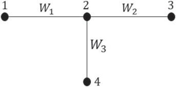
Example 4.2.

Consider the tree T₁ in Figure 1, where the edge weights are $$\begin{array}{c}{W}_1=\left[\begin{array}{cc}1& 0\\ 0& 1\end{array}\right],\mathrm{\hspace{1em}}\mathrm{\hspace{1em}}{W}_2=\left[\begin{array}{cc}2& 0\\ 0& 1\end{array}\right],\\ W_3=\left[\begin{array}{cc}1& 0\\ 0& 2\end{array}\right].\end{array}$$

Fig. 1 Tree T₁ on 4 vertices.

Then, $$\begin{array}{c}\Delta =\left[\begin{array}{cccc}0& W_1^2& {(W_1+W_2)}^2& {(W_1+W_3)}^2\\ W_1^2& 0& W_2^2& W_3^2\\ {(W_1+W_2)}^2& W_2^2& 0& {(W_2+W_3)}^2\\ {(W_1+W_3)}^2& W_3^2& {(W_2+W_3)}^2& 0\end{array}\right]=\left[\begin{array}{cccccccc}0& 0& 1& 0& 9& 0& 4& 0\\ 0& 0& 0& 1& 0& 4& 0& 9\\ 1& 0& 0& 0& 4& 0& 1& 0\\ 0& 1& 0& 0& 0& 1& 0& 4\\ 9& 0& 4& 0& 0& 0& 9& 0\\ 0& 4& 0& 1& 0& 0& 0& 9\\ 4& 0& 1& 0& 9& 0& 0& 0\\ 0& 9& 0& 4& 0& 9& 0& 0\end{array}\right] \text{and}\\ \sum _{i=1}^4\frac{{\widehat{{\delta }_i}}^2}{{\tau }_i}=W_1^2+W_2^2+W_3^2-{(W_1+W_2+W_3)}^2=\left[\begin{array}{cc}-10& 0\\ 0& -10\end{array}\right].\end{array}$$

One can verify that, $$\begin{array}{c}\det (\Delta )=102400={(-1)}^6{2}^6\prod _{i=1}^4{({\tau }_i)}^2\prod _{i=1}^3\det (W_i{}^2)\\ \det \left(\sum _{i=1}^4\frac{{\widehat{{\delta }_i}}^2}{{\tau }_i}\right).\end{array}$$

Next, we obtain a formula for the determinant of the squared distance matrix of a tree T, which has exactly one vertex of degree 2.

Theorem 4.3.

Let T be a tree on n vertices with the edge set $E(T)=\{e_1,e_2,\dots ,e_{n-1}\}$. Let the positive definite matrices $W_1,W_2,\dots ,W_{n-1}$ of order s be the weights of the edges $e_1,e_2,\dots ,e_{n-1}$, respectively. Let v be the vertex of degree 2 and u and w be its neighbors in T. If $e_i=(u,v)$ and $e_j=(v,w)$, then $$\begin{array}{c}\det (\Delta )={(-1)}^{(n-1)s}{2}^{(2n-5)s}\det {(W_i+W_j)}^2\prod _{k=1}^{n-1}\\ \det (W_k^2)\prod _{k\ne v}{\tau }_k^s.\end{array}$$

Proof.

Let us assign an orientation to each edge of T. Without loss of generality, assume that, the edge e_i is directed from u to v and the edge e_j is directed from v to w.

Let Δ_i denote the i-th column block of the block matrix Δ. Let t_i be the $n\times 1$ column vector with 1 at the i-th position and 0 elsewhere, $i=1,2,\dots ,n$. Therefore, by using Lemma 3.2, we have $$\begin{array}{c}\left[\begin{array}{c}{Q}^{\prime }\otimes I_s\\ t_v^{\prime }\otimes I_s\end{array}\right]\Delta \left[\begin{array}{cc}Q\otimes I_s& t_v\otimes I_s\end{array}\right]\hspace{1em}\\ =\left[\begin{array}{cc}(Q^{\prime }\otimes I_s)\Delta (Q\otimes I_s)& (Q^{\prime }\otimes I_s){\Delta }_v\\ {\Delta }_v^{\prime }(Q\otimes I_s)& 0\end{array}\right]\hspace{1em}\\ =\left[\begin{array}{cc}-2F(H\otimes I_s)F)& (Q^{\prime }\otimes I_s){\Delta }_v\\ {\Delta }_v^{\prime }(Q\otimes I_s)& 0\end{array}\right]\end{array}$$

Pre-multiplying and post-multiplying the above equation by $\left[\begin{array}{cc}{F}^{-1}& 0\\ 0& I_s\end{array}\right]$, we get $$\begin{array}{c}\left[\begin{array}{cc}{F}^{-1}& 0\\ 0& I_s\end{array}\right]\left[\begin{array}{c}{Q}^{\prime }\otimes I_s\\ t_v^{\prime }\otimes I_s\end{array}\right]\Delta \left[\begin{array}{cc}Q\otimes I_s& t_v\otimes I_s\end{array}\right]\left[\begin{array}{cc}{F}^{-1}& 0\\ 0& I_s\end{array}\right]\\ =\left[\begin{array}{cc}-2(H\otimes I_s)& F^{-1}(Q^{\prime }\otimes I_s){\Delta }_v\\ {\Delta }_v^{\prime }(Q\otimes I_s)F^{-1}& 0\end{array}\right],\end{array}$$

which implies that $$\begin{array}{c}{(\det (F^{-1}))}^2\det (\Delta )\\ \hspace{1em}=\det \left[\begin{array}{cc}-2(H\otimes I_s)& F^{-1}(Q^{\prime }\otimes I_s){\Delta }_v\\ {\Delta }_v^{\prime }(Q\otimes I_s)F^{-1}& 0\end{array}\right].\end{array}$$

Let $H(j|j)$ denote the $(n-2)s\times (n-2)s$ submatrix obtained by deleting the all blocks in the j-th row and j-th column from $H\otimes I_s$. Let $G(j|j)$ denote the $(n-2)s\times s$ submatrix obtained by deleting the j-the block in $F^{-1}(Q^{\prime }\otimes I_s){\Delta }_v$. Let R_i and C_i denote the i-th row and i-th column of the matrix $\left[\begin{array}{cc}-2(H\otimes I_s)& F^{-1}(Q^{\prime }\otimes I_s){\Delta }_v\\ {\Delta }_v^{\prime }(Q\otimes I_s)F^{-1}& 0\end{array}\right]$, respectively. Note that the blocks in the i-th and j-th column of $H\otimes I_s$ are identical. Now, perform the operations $R_j-R_i$ and $C_j-C_i$ in $\left[\begin{array}{cc}-2(H\otimes I_s)& F^{-1}(Q^{\prime }\otimes I_s){\Delta }_v\\ {\Delta }_v^{\prime }(Q\otimes I_s)F^{-1}& 0\end{array}\right]$, and then interchange R_j and $R_{n-1}$, C_j and $C_{n-1}$. Since ${\Delta }_v^{\prime }(Q\otimes I_s)F^{-1}{)}_j-{({\Delta }_v^{\prime }(Q\otimes I_s)F^{-1})}_i=-W_j-W_i$, therefore $$\begin{array}{c}\det \left[\begin{array}{cc}-2(H\otimes I_s)& F^{-1}(Q^{\prime }\otimes I_s){\Delta }_v\\ {\Delta }_v^{\prime }(Q\otimes I_s)F^{-1}& 0\end{array}\right]\\ \hspace{1em}=\det \left[\begin{array}{ccc}-2H(j|j)& 0& G(j|j)\\ 0& 0& -W_j-W_i\\ G{(j|j)}^{\prime }& -W_j-W_i& 0\end{array}\right].\end{array}$$

Since $H(j|j)$ is the edge orientation matrix of the tree obtained by deleting the vertex v and replacing the edges e_i and e_j by a single edge directed from u to w in the tree, by Theorem 2.1, we have $\det (H(j|j)=2^{(n-3)s}\prod _{k\ne v}{\tau }_k^s$, which is nonzero. Therefore, by applying the Schur complement formula, we have $$\begin{array}{c} \det \left[\begin{array}{ccc}-2H(j|j)& 0& G(j|j)\\ 0& 0& -W_j-W_i\\ G{(j|j)}^{\prime }& -W_j-W_i& 0\end{array}\right]\\ =\det (-2H(j|j))\det (\left[\begin{array}{cc}0& -W_j-W_i\\ -W_j-W_i& 0\end{array}\right](\\ -\left[\begin{array}{cc}0& 0\\ 0& G{(j|j)}^{\prime }{(-2H(j|j))}^{-1}G(j|j)\end{array}\right])\\ ={(-2)}^{(n-2)s}\det (H(j|j))\\ \det \left[\begin{array}{cc}0& -W_j-W_i\\ -W_j-W_i& -G{(j|j)}^{\prime }{(-2H(j|j))}^{-1}G(j|j)\end{array}\right].\end{array}$$

Again, by the proof of Theorem 4.1, we have $$G{(j|j)}^{\prime }{(-2H(j|j))}^{-1}G(j|j)=-\frac{1}{4}\sum _{i\ne v}\frac{{\widehat{{\delta }_i}}^2}{{\tau }_i}.$$

Therefore, $$\begin{array}{c}\det \left[\begin{array}{ccc}-2H(j|j)& 0& G(j|j)\\ 0& 0& -W_j-W_i\\ G{(j|j)}^{\prime }& -W_j-W_i& 0\end{array}\right]\\ ={(-2)}^{(n-2)s}\det (H(j|j))\det \left[\begin{array}{cc}0& -W_j-W_i\\ -W_j-W_i& \frac{1}{4}\sum _{i\ne v}\frac{{\widehat{{\delta }_i}}^2}{{\tau }_i}\end{array}\right]\\ ={(-2)}^{(n-2)s}\det (H(j|j))\det \left[\begin{array}{cc}0& W_j+W_i\\ W_j+W_i& -\frac{1}{4}\sum _{i\ne v}\frac{{\widehat{{\delta }_i}}^2}{{\tau }_i}\end{array}\right].\end{array}$$

Since $\det (-\frac{1}{4}\sum _{i\ne v}\frac{{\widehat{{\delta }_i}}^2}{{\tau }_i})\ne 0$, by Schur complement formula, we have $$\begin{array}{c}\det \left[\begin{array}{cc}0& W_j+W_i\\ W_j+W_i& -\frac{1}{4}\sum _{i\ne v}\frac{{\widehat{{\delta }_i}}^2}{{\tau }_i}\end{array}\right]\\ =\det (-\frac{1}{4}\sum _{i\ne v}\frac{{\widehat{{\delta }_i}}^2}{{\tau }_i})\\ \det [0-(W_j+W_i){(-\frac{1}{4}\sum _{i\ne v}\frac{{\widehat{{\delta }_i}}^2}{{\tau }_i})}^{-1}(W_j+W_i)]\\ ={(-1)}^s\det (-\frac{1}{4}\sum _{i\ne v}\frac{{\widehat{{\delta }_i}}^2}{{\tau }_i})\\ \det {(-\frac{1}{4}\sum _{i\ne v}\frac{{\widehat{{\delta }_i}}^2}{{\tau }_i})}^{-1}\det {(W_j+W_i)}^2\\ ={(-1)}^s\det {(W_i+W_j)}^2.\end{array}$$

Thus, $$\begin{array}{c}\det (\Delta )={(\det F)}^2{(-1)}^s{(-2)}^{(n-2)s}{2}^{(n-3)s}\\ \prod _{k\ne v}{\tau }_k^s \det {(W_i+W_j)}^2\\ ={(-1)}^{(n-1)s}{2}^{(2n-5)s}\det {(W_i+W_j)}^2\\ \prod _{k=1}^{n-1}\det (W_k^2)\prod _{k\ne v}{\tau }_k^s.\end{array}$$

This completes the proof. □

Now, we illustrate the above theorem by the following example.

Example 4.4.

Consider the tree T₂ in Figure 2, where the edge weights are $$\begin{array}{c}{W}_1=\left[\begin{array}{cc}1& 0\\ 0& 1\end{array}\right],\mathrm{\hspace{1em}}\mathrm{\hspace{1em}}{W}_2=\left[\begin{array}{cc}2& 0\\ 0& 1\end{array}\right],\\ W_3=\left[\begin{array}{cc}1& 0\\ 0& 2\end{array}\right],\mathrm{\hspace{1em}}\mathrm{\hspace{1em}}{W}_4=\left[\begin{array}{cc}2& 0\\ 0& 2\end{array}\right].\end{array}$$

Fig. 2 Tree T₂ on 5 vertices.

Then, $$\Delta =\left[\begin{array}{ccccc}0& W_1^2& {(W_1+W_2)}^2& {(W_1+W_2+W_3)}^2& {(W_1+W_2+W_4)}^2\\ W_1^2& 0& W_2^2& {(W_2+W_3)}^2& {(W_2+W_4)}^2\\ {(W_1+W_2)}^2& W_2^2& 0& W_3^2& W_4^2\\ {(W_1+W_2+W_3)}^2& {(W_2+W_3)}^2& W_3^2& 0& {(W_3+W_4)}^2\\ {(W_1+W_2+W_4)}^2& {(W_2+W_4)}^2& W_4^2& {(W_3+W_4)}^2& 0\end{array}\right]$$ $$=\left[\begin{array}{cccccccccc}0& 0& 1& 0& 9& 0& 16& 0& 25& 0\\ 0& 0& 0& 1& 0& 4& 0& 16& 0& 16\\ 1& 0& 0& 0& 4& 0& 9& 0& 16& 0\\ 0& 1& 0& 0& 0& 1& 0& 9& 0& 9\\ 9& 0& 4& 0& 0& 0& 1& 0& 4& 0\\ 0& 4& 0& 1& 0& 0& 0& 4& 0& 4\\ 16& 0& 9& 0& 1& 0& 0& 0& 9& 0\\ 0& 16& 0& 9& 0& 4& 0& 0& 0& 16\\ 25& 0& 16& 0& 4& 0& 9& 0& 0& 0\\ 0& 16& 0& 9& 0& 4& 0& 16& 0& 0\end{array}\right].$$

One can verify that, $$\begin{array}{c}\det (\Delta )=9437184={(-1)}^8{2}^{10}\det {(W_1+W_2)}^2\\ \prod _{i=1}^4\det (W_i^2)\prod _{k\ne 2}{\tau }_k^s.\end{array}$$

Corollary 4.5.

Let T be a tree on n vertices and each edge e_i of T is assigned a positive definite matrix W_i order s, $i=1,2,\dots ,n-1$. If T has at least two vertices of degree 2, then $\det (\Delta )=0$.

Proof.

Let T be a tree with at least two vertices v₁ and v₂ of degree 2. Therefore, ${\tau }_{v_1}=2-{\delta }_{v_1}=2-2=0$ and ${\tau }_{v_2}=2-{\delta }_{v_2}=2-2=0$. Let u and w be the neighbours of v₁ and $e_i=(u,v_1)$ and $e_j=(v_1,w)$. Therefore, by Theorem 4.3, we have $$\begin{array}{c}\det (\Delta )={(-1)}^{(n-1)s}{2}^{(2n-5)s}\det {(W_i+W_j)}^2\\ \prod _{k=1}^{n-1}\det (W_k^2)\prod _{k\ne v_1}{\tau }_k^s.\end{array}$$

Since ${\tau }_{v_2}=0$, therefore $\det (\Delta )=0$. This completes the proof. □

5 Inverse of the squared distance matrix

This section considers trees with no vertex of degree 2 and obtains an explicit formula for the inverse of its squared distance matrix. First, let us prove the following lemma which will be used to find ${\Delta }^{-1}$.

Lemma 5.1.

Let T be a tree of order n with no vertex of degree 2 and each edge of T is assigned a positive definite matrix weight of order s. If $\beta =\widehat{{\delta }^{\prime }}(\widehat{\tau }\otimes I_s)\widehat{\delta }$ and $\eta =2\tau \otimes I_s-L(\widehat{\tau }\otimes I_s)\widehat{\delta }$, then $$\Delta \eta ={\mathbf{1}}_n\otimes \beta .$$

Proof.

By Lemma 3.3, we have $\Delta L=2D(\tilde{\tau }\otimes I_s)-{\mathbf{1}}_n\otimes \widehat{\delta }\prime$. Hence, $$\begin{array}{c}\Delta L(\widehat{\tau }\otimes I_s)\widehat{\delta }=2D\widehat{\delta }-({\mathbf{1}}_n\otimes \widehat{\delta }\prime )(\widehat{\tau }\otimes I_s)\widehat{\delta }\\ =2D\widehat{\delta }-{\mathbf{1}}_n\otimes \sum _{i=1}^n\frac{{\widehat{{\delta }_i}}^2}{{\tau }_i}.\end{array}$$

Since $\beta =\widehat{{\delta }^{\prime }}(\widehat{\tau }\otimes I_s)\widehat{\delta }={\sum }_{i=1}^n\frac{{\widehat{{\delta }_i}}^2}{{\tau }_i}$, therefore $\Delta L(\widehat{\tau }\otimes I_s)\widehat{\delta }=2D\widehat{\delta }-{\mathbf{1}}_n\otimes \beta$. By Lemma 3.1, we have $\Delta (\tau \otimes I_s)=D\widehat{\delta }$ and hence $\Delta L(\widehat{\tau }\otimes I_s)\widehat{\delta }=2\Delta (\tau \otimes I_s)-{\mathbf{1}}_n\otimes \beta$. This completes the proof. □

If the tree T has no vertex of degree 2 and $\det (\beta )\ne 0$, then Δ is nonsingular, that is, ${\Delta }^{-1}$ exists. In the next theorem, we determine the formula for ${\Delta }^{-1}$.

Theorem 5.2.

Let T be a tree of order n with no vertex of degree 2 and each edge of T is assigned a positive definite matrix weight of order s. Let $\beta =\widehat{{\delta }^{\prime }}(\widehat{\tau }\otimes I_s)\widehat{\delta }$ and $\eta =2\tau \otimes I_s-L(\widehat{\tau }\otimes I_s)\widehat{\delta }$. If $\det (\beta )\ne 0$, then $${\Delta }^{-1}=-\frac{1}{4}L(\widehat{\tau }\otimes I_s)L+\frac{1}{4}\eta {\beta }^{-1}{\eta }^{\prime }.$$

Proof.

Let $X=-\frac{1}{4}L(\widehat{\tau }\otimes I_s)L+\frac{1}{4}\eta {\beta }^{-1}{\eta }^{\prime }$. Then, (3) $$\Delta X=-\frac{1}{4}\Delta L(\widehat{\tau }\otimes I_s)L+\frac{1}{4}\Delta \eta {\beta }^{-1}{\eta }^{\prime }.$$(3)

By Lemma 3.3, we have $\Delta L=2D(\tilde{\tau }\otimes I_s)-{\mathbf{1}}_n\otimes \widehat{\delta }\prime$. Therefore, $$\Delta L(\widehat{\tau }\otimes I_s)L=2DL-({\mathbf{1}}_n\otimes \widehat{\delta }\prime )(\widehat{\tau }\otimes I_s)L.$$

By Theorem 2.2, $DL={\mathbf{1}}_n{\tau }^{\prime }\otimes I_s-2I_n\otimes I_s$ and hence (4) $$\Delta L(\widehat{\tau }\otimes I_s)L=2({\mathbf{1}}_n{\tau }^{\prime }\otimes I_s-2I_n\otimes I_s)-({\mathbf{1}}_n\otimes \widehat{\delta }\prime )(\widehat{\tau }\otimes I_s)L.$$(4)

By Lemma 5.1, we have $\Delta \eta ={\mathbf{1}}_n\otimes \beta =({\mathbf{1}}_n\otimes I_s)\beta$. Therefore, from equation (3)(3) $$\Delta X=-\frac{1}{4}\Delta L(\widehat{\tau }\otimes I_s)L+\frac{1}{4}\Delta \eta {\beta }^{-1}{\eta }^{\prime }.$$(3) and (4)(4) $$\Delta L(\widehat{\tau }\otimes I_s)L=2({\mathbf{1}}_n{\tau }^{\prime }\otimes I_s-2I_n\otimes I_s)-({\mathbf{1}}_n\otimes \widehat{\delta }\prime )(\widehat{\tau }\otimes I_s)L.$$(4) , we have $$\begin{array}{c}\Delta X=-\frac{1}{2}({\mathbf{1}}_n{\tau }^{\prime }\otimes I_s-2I_n\otimes I_s)\\ + \frac{1}{4}({\mathbf{1}}_n\otimes \widehat{\delta }\prime )(\widehat{\tau }\otimes I_s)L\\ + \frac{1}{4}({\mathbf{1}}_n\otimes I_s){\eta }^{\prime }\\ =-\frac{1}{2}{\mathbf{1}}_n{\tau }^{\prime }\otimes I_s+I_n\otimes I_s+\frac{1}{4}({\mathbf{1}}_n\otimes \widehat{\delta }\prime )(\widehat{\tau }\otimes I_s)L\\ + \frac{1}{4}({\mathbf{1}}_n\otimes I_s){(2\tau \otimes I_s-L(\widehat{\tau }\otimes I_s)\widehat{\delta })}^{\prime }\\ =-\frac{1}{2}{\mathbf{1}}_n{\tau }^{\prime }\otimes I_s+I_n\otimes I_s+\frac{1}{4}({\mathbf{1}}_n\otimes \widehat{\delta }\prime )(\widehat{\tau }\otimes I_s)L\\ + \frac{1}{4}({\mathbf{1}}_n\otimes I_s)(2{\tau }^{\prime }\otimes I_s-{\widehat{\delta }}^{\prime }(\widehat{\tau }\otimes I_s)L)\\ =I_n\otimes I_s=I_{ns}.\end{array}$$

This completes the proof. □

Now, let us illustrate the above formula for ${\Delta }^{-1}$ by an example.

Example 5.3.

Consider the tree T₁ in Figure 1, where the edge weights are $$\begin{array}{c}{W}_1=\left[\begin{array}{cc}1& 0\\ 0& 1\end{array}\right],\mathrm{\hspace{1em}}\mathrm{\hspace{1em}}{W}_2=\left[\begin{array}{cc}2& 0\\ 0& 1\end{array}\right],\\ W_3=\left[\begin{array}{cc}1& 0\\ 0& 2\end{array}\right].\end{array}$$

Then, $$\begin{array}{c}\Delta =\left[\begin{array}{cccc}0& W_1^2& {(W_1+W_2)}^2& {(W_1+W_3)}^2\\ W_1^2& 0& W_2^2& W_3^2\\ {(W_1+W_2)}^2& W_2^2& 0& {(W_2+W_3)}^2\\ {(W_1+W_3)}^2& W_3^2& {(W_2+W_3)}^2& 0\end{array}\right]\\ =\left[\begin{array}{cccccccc}0& 0& 1& 0& 9& 0& 4& 0\\ 0& 0& 0& 1& 0& 4& 0& 9\\ 1& 0& 0& 0& 4& 0& 1& 0\\ 0& 1& 0& 0& 0& 1& 0& 4\\ 9& 0& 4& 0& 0& 0& 9& 0\\ 0& 4& 0& 1& 0& 0& 0& 9\\ 4& 0& 1& 0& 9& 0& 0& 0\\ 0& 9& 0& 4& 0& 9& 0& 0\end{array}\right],\\ L=\left[\begin{array}{cccc}{W}_1^{-1}& -W_1^{-1}& 0& 0\\ -W_1^{-1}& W_1^{-1}+W_2^{-1}+W_3^{-1}& -W_2^{-1}& -W_3^{-1}\\ 0& -W_2^{-1}& W_2^{-1}& 0\\ 0& -W_3^{-1}& 0& W_3^{-1}\end{array}\right]\\ =\left[\begin{array}{cccccccc}1& 0& -1& 0& 0& 0& 0& 0\\ 0& 1& 0& -1& 0& 0& 0& 0\\ -1& 0& 2.5& 0& -0.5& 0& -1& 0\\ 0& -1& 0& 2.5& 0& -1& 0& -0.5\\ 0& 0& -0.5& 0& 0.5& 0& 0& 0\\ 0& 0& 0& -1& 0& 1& 0& 0\\ 0& 0& -1& 0& 0& 0& 1& 0\\ 0& 0& 0& -0.5& 0& 0& 0& 0.5\end{array}\right],\\ \beta =\sum _{i=1}^4\frac{{\widehat{{\delta }_i}}^2}{{\tau }_i}=W_1^2+W_2^2+W_3^2-{(W_1+W_2+W_3)}^2\\ =\left[\begin{array}{cc}-10& 0\\ 0& -10\end{array}\right], \text{and}\\ {\eta }^{\prime }=\left[\begin{array}{cccccccc}-3& 0& 11& 0& -1& 0& -3& 0\\ 0& -3& 0& 11& 0& -3& 0& -1\end{array}\right].\end{array}$$

Therefore, $$\begin{array}{c}L(\widehat{\tau }\otimes I_s)L=\left[\begin{array}{cccccccc}0& 0& 1.5& 0& -0.5& 0& -1& 0\\ 0& 0& 0& 1.5& 0& -1& 0& -0.5\\ 1.5& 0& -4& 0& 1& 0& 1.5& 0\\ 0& 1.5& 0& -4& 0& 1.5& 0& 1\\ -0.5& 0& 1& 0& 0& 0& -0.5& 0\\ 0& -1& 0& 1.5& 0& 0& 0& -0.5\\ -1& 0& 1.5& 0& -0.5& 0& 0& 0\\ 0& -0.5& 0& 1& 0& -0.5& 0& 0\end{array}\right], \text{and}\\ \eta {\beta }^{-1}{\eta }^{\prime }=\left[\begin{array}{cccccccc}-0.9& 0& 3.3& 0& -0.3& 0& -0.9& 0\\ 0& -0.9& 0& 3.3& 0& -0.9& 0& -0.3\\ 3.3& 0& -12.1& 0& 1.1& 0& 3.3& 0\\ 0& 3.3& 0& -12.1& 0& 3.3& 0& 1.1\\ -0.3& 0& 1.1& 0& -0.1& 0& -0.3& 0\\ 0& -0.9& 0& 3.3& 0& -0.9& 0& -0.3\\ -0.9& 0& 3.3& 0& -0.3& 0& -0.9& 0\\ 0& -0.3& 0& 1.1& 0& -0.3& 0& -0.1\end{array}\right].\end{array}$$

One can verify that, $${\Delta }^{-1}=-\frac{1}{4}L(\widehat{\tau }\otimes I_s)L+\frac{1}{4}\eta {\beta }^{-1}{\eta }^{\prime }.$$

Acknowledgments

We are indebted to the referee for their valuable comments and suggestions.

References

- Atik, F., Bapat, R. B., Kannan, M. R. (2019). Resistance matrices of graphs with matrix weights. Linear Algebra Appl. 571: 41–57.
- Atik, F., Kannan, M. R., Bapat, R. B. (2021). On distance and Laplacian matrices of trees with matrix weights. Linear and Multilinear Algebra. 69(14): 2607–2619.
- Bapat, R. B. (2006). Determinant of the distance matrix of a tree with matrix weights. Linear Algebra Appl. 416(1): 2–7.
- Bapat, R. B. (2010). Graphs and Matrices, Vol. 27. London: Springer.
- Bapat, R. B. (2019). Squared distance matrix of a weighted tree. Electron. J. Graph Theory Appl. (EJGTA). 7(2): 301–313.
- Bapat, R. B., Sivasubramanian, S. (2015). Product distance matrix of a tree with matrix weights. Linear Algebra Appl. 468: 145–153.
- Bapat, R. B., Sivasubramanian, S. (2016). Squared distance matrix of a tree: inverse and inertia. Linear Algebra Appl. 491: 328–342.
- Bapat, R. B., Sivasubramanian, S. (2013). Product distance matrix of a graph and squared distance matrix of a tree. Appl. Anal. Discrete Math. 7(2): 285–301.
- Das, J., Mohanty, S. (2020). On squared distance matrix of complete multipartite graphs. arXiv preprint arXiv:2012.04341.
- Ganesh, S., Mohanty, S. (2022). Trees with matrix weights: Laplacian matrix and characteristic-like vertices. Linear Algebra Appl. 646: 195–237.
- Hansen, J. (2021). Expansion in matrix-weighted graphs. Linear Algebra Appl. 630: 252–273.
- Horn, R. A., Johnson, C. R. (1994). Topics in Matrix analysis. Cambridge: Cambridge University Press, Corrected reprint of the 1991 original.