
 ?Mathematical formulae have been encoded as MathML and are displayed in this HTML version using MathJax in order to improve their display. Uncheck the box to turn MathJax off. This feature requires Javascript. Click on a formula to zoom.
Abstract
Given a signed graph , let
and
be its standard adjacency matrix and the diagonal matrix of net-degrees, respectively. The net Laplacian matrix of
is defined as
. In this paper we investigate signed graphs whose net Laplacian spectrum consists entirely of integers. The focus is mainly on the two extreme cases, the one in which all eigenvalues of
are simple and the other in which
has 2 or 3 (distinct) eigenvalues. Both cases include structure theorems, degree constraints and particular constructions of new examples. Several applications in the framework of control theory are reported.
1 Introduction
A signed graph is a pair
, where
is an (unsigned) graph, called the underlying graph, and
is the sign function. The edge set of a signed graph is composed of subsets of positive and negative edges. We denote the number of vertices (also known as the order) of a signed graph by n. In literature, one may find a slightly different notation with Γ or Σ for a signed graph. Our dot-notation appears in papers concerning spectra, where the absence of a dot refers to the underlying graph simultaneously interpreting a signed graph with all-positive signature.
Many familiar notions about graphs extend directly to the domain of signed graphs. For example, the degree du
of a vertex u of is its degree in G. Similarly, a signed graph is regular if its underlying graph is regular. On the other hand, there are some notions exclusive to signed graphs. The positive degree
is the number of positive neighbors of u (i.e. those adjacent to u by a positive edge). In a similar way, we define the negative degree
. The net-degree of u is defined as
. A signed graph is said to be net-regular if the net-degree, considered as a function on the vertex set, is constant.
The adjacency matrix of
is obtained from the standard adjacency matrix of G by replacing + 1 with –1 whenever the corresponding edge is negative. The Laplacian matrix is defined as
, where
is the diagonal matrix of vertex degrees.
The net Laplacian matrix is defined as , where
is the diagonal matrix of net-degrees. The matrices
and
have received a great deal of attention in the theory of spectra of signed graphs. On the contrary, the net Laplacian appears very sporadically, say in [Citation7, Citation13, Citation15–17]. The authors of [Citation7] highlighted its significance in the study of controllability of undirected signed graphs. To the best of our knowledge, the first appearance of the term ‘net Laplacian’ is recorded in [Citation16]. Evidently, in particular case of unsigned graphs the net Laplacian coincides with the Laplacian.
We denote the eigenvalues (with possible repetitions) of by
. The eigenvalues, the spectrum and the eigenvectors of
are simultaneously considered as the net Laplacian eigenvalues, the net Laplacian spectrum and the net Laplacian eigenvectors of
, but to ease language, except in the formulations of the statements, we suppress the prefix ‘net Laplacian’ from the previous terminology. In addition, we write ‘
has k eigenvalues’ to mean that
has k distinct eigenvalues. It is not difficult to see that 0 is an eigenvalue of every signed graph with the all-1 eigenvector.
We say that the spectrum of is integral if it consists entirely of integers. When this occurs, we also say that
is integral. Such signed graphs are subject of the research reported in this paper. In particular, we consider the case in which
has no repeated eigenvalues and its counterpart in which the number of eigenvalues of
is extremely small; precisely, equal to 2 or 3. In both cases we establish some theoretical results concerning the structure of signed graphs under consideration, and then provide particular constructions. An application of integral signed graphs without repeated eigenvalues in the framework of control theory is investigated.
The paper is organized as follows. Section 2 contains some additional terminology and notation, along with some known results. In particular, one can find definition of the class of integral signed graphs called ∇-cographs and the particular subclass of ∇-threshold graphs. In Section 3 we investigate the spectrum of ∇-cographs and give constructions of those that avoid repeated eigenvalues. All connected signed graphs with 2 eigenvalues and at most 8 vertices are reported in Section 4; all of them are integral. Structural examinations of certain signed graphs with 2 or 3 eigenvalues are given in Section 5. Finally, some applications in control theory are separated in Section 6.
2 Preparatory
We use j, , J and I to denote the all-1 vector, the all-0 vector, the all-1 matrix and the identity matrix, respectively. The length or the size may be given in the subscript. We write
to denote the Euclidean inner product of the vectors x and y. For the signed graphs
and
denotes their disjoint union, and
the disjoint union of k copies of
. The negation
of
is obtained by reversing the sign of every edge of
. Evidently,
acts as the net Laplacian matrix of
, and the spectrum of
is obtained by negating every eigenvalue of
. Finally, if
and
are isomorphic, we write
. For the undefined notions, we refer the reader to [Citation18].
The join of (unsigned) graphs G1, G2 is obtained by inserting an edge between every vertex of
and every vertex of
. In the framework of signed graphs we have similar definitions. For the signed graphs
, the positive join (resp. negative join)
(
) is obtained by inserting a positive (negative) edge between every vertex of
and every vertex of
.
We recall from [Citation10] that an unsigned cograph is iteratively defined in the following way: K1 is a cograph; if G1, G2 are cographs, then is a cograph. Alternatively, a cograph is a P4-free graph. Similarly, a threshold graph
is defined on the basis of its binary generating sequence
in the following way:
; if
is already constructed, then
is formed by adding a vertex non-adjacent to the vertices of
if bi
= 0 or by adding a vertex adjacent to all the vertices of
if bi
= 1. Alternatively, a threshold graph is a
-free graph, and so every threshold graph is a cograph. For more details see [Citation9].
In the framework of signed graphs we may define a signed cograph (resp. signed threshold graph) as a signed graph whose underlying graph is a cograph (threshold graph). However, in this study we are more interested in particular classes so called ∇-cographs. A ∇-cograph is a signed graph defined in the following way: K1 is a ∇-cograph; if are ∇-cographs, then
and
are ∇-cographs. Similarly, a ∇-threshold graph is defined on the basis of its
-generating sequence
as follows:
is a ∇-threshold graph and if
is already constructed, then
is formed by adding a vertex non-adjacent to the vertices of
if bi
= 0, or adding a vertex joined by a positive edge to all the vertices of
if bi
= 1, or adding a vertex joined by a negative edge to all the vertices of
if
. Observe that a ∇-threshold graph does not depend on the choice for b1 and it is uniquely determined by the remainder of b.
Remark 1.
Evidently, every ∇-cograph is a signed cograph and every ∇-threshold graph is a signed threshold graph (and consequently, it is a signed cograph). The prefix ∇ suggests that the sign of every edge is determined by the positive or the negative join operation.
In this paper we will frequently use the following result of [Citation15]. It is a ‘signed’ generalization of the known result obtained by Merris [Citation10] (see also [Citation11]).
Theorem 2.1.
[Citation15, Theorem 3] Let and
be signed graphs with net Laplacian eigenvalues
and
, respectively, and let
be a fixed element of
. The net Laplacian eigenvalues of
are
and 0.
If x is a net Laplacian eigenvector of orthogonal to j and associated with a net Laplacian eigenvalue ν, then its extension defined to be zero on each vertex of
is a net Laplacian eigenvector of
associated with
, and similarly for the net Laplacian eigenvectors of
that arise from those of
. The net Laplacian eigenvalue
is associated with the net Laplacian eigenvector with weight
on each vertex of
and n1 on each vertex of
.
As observed in [Citation14], an immediate consequence of the previous theorem is the fact that the largest eigenvalue of a signed graph with n vertices does not exceed n, and it attains n if and only if
is a positive join of two signed graphs.
We conclude this section with a simple corollary treating ∇-thresholds graphs.
Corollary 2.2.
Let be a ∇-threshold graph generated by the sequence
with
. For t = 0,
is a positive (for bk = 1) or a negative (for
) join and its net Laplacian spectrum is formed as in Theorem 2.1. For t > 0,
is a disjoint union of a connected ∇-threshold graph
generated by
and the set of t isolated vertices. The net Laplacian spectrum of
consists of the net Laplacian eigenvalues of
obtained as in Theorem 2.1 and t zeroes.
Proof.
For t = 0, the result follows immediately from definition of a ∇-threshold graph and Theorem 2.1.
For t > 0, we have , and thus the spectrum of
consists of the eigenvalues of
and the eigenvalues of tK1 (zero with multiplicity t). In addition,
implies that
is connected. Moreover, it is a positive or a negative join (depending on the sign of bk
), and so its eigenvalues are obtained as in Theorem 2.1. □
3 Spectrum of ∇-cographs
As we said in the first section, the spectrum of the net Laplacian matrix is studied in just few references. Some particular results (including small structural perturbations, relations with the spectrum of the standard Laplacian matrix and certain operations on signed graphs) can be found in [Citation15, Citation17]. In this section we establish some spectral properties of ∇-cographs and the subclass of ∇-threshold graphs. We devote a particular attention to those that have no repeated eigenvalues.
First, every ∇-cograph (as well as every ∇-threshold graph) is integral. To see this, one may suppose that is the smallest connected non-integral ∇-cograph and then use Theorem 2.1 to show that it contains a connected ∇-cograph with smaller order which must be non-integral. In what follows we prove that the class of all ∇-threshold graphs does not contain two that share the same spectrum.
Theorem 3.1.
No two ∇-threshold graphs have the same net Laplacian spectrum.
Proof.
Assume for the sake of contradiction that make a smallest pair (relative to the number of vertices) of ∇-threshold graphs with the same spectrum. Let n be their common order.
Let first be disconnected. Hence, we have
, where
is a connected ∇-threshold graph with
vertices. Without loss of generality, we may suppose that
is a positive join, and in this case k is the largest eigenvalue of
, by Corollary 2.2. In addition, the least eigenvalue of
is greater than – k. Consequently, we have the same situation for
: its largest eigenvalue is k and its spectrum is bounded from below by
. Since k < n, we get that
is disconnected, as well; otherwise, one of
would appear in its spectrum. Therefore, we have
, where
is a connected ∇-threshold graph. Moreover, k is an eigenvalue of
and its least eigenvalue is greater than – k (as
and
share the same spectrum). In other words,
is a positive join and has k vertices, which implies c1 = c2, which further implies that
and
share the same spectrum, but this contradicts the assumption that
make a smallest such a pair.
Let now be connected and, without loss of generality, let it be a positive join. By Corollary 2.2, the order of
appears as a common eigenvalue of
and
, which implies that
is also a positive join. In other words, we have
and
for some ∇-threshold graphs
. If
are the common eigenvalues of
and
, then the eigenvalues of
and
are
and 0 (by Corollary 2.2, as well). In other words,
and
share the same spectrum, which as before contradicts the initial assumption on minimality of
and
. This completes the proof. □
On the basis of Theorem 2.1 (and Corollary 2.2) we can give a simple algorithm that computes the eigenvalues and the eigenvectors of a ∇-threshold graph. Its correctness is inspected directly, by employing the previous results.
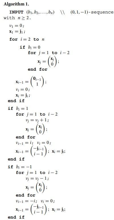
RETURN
Eigenvalues and eigenvectors.
The algorithm contains a linear loop which in each iteration includes another linear loop, so the time complexity is quadratic. We now extend a rooted tree representation of cographs of [Citation4] to ∇-cographs. For a ∇-cograph , the root and every interior vertex of the corresponding tree
, called a ∇-cotree, is either of 0-type (corresponding to disjoint union), or (+)-type (corresponding to positive join), or (–)-type (corresponding to negative join). The terminal vertices (leaves) are typeless and each of them represents itself in
. Unless
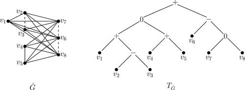
consists of an isolated vertex, the root and every interior vertex have at least two direct successors. Moreover, every non-terminal direct successor of any vertex v has a type that differs from the type of v. It can be easily seen that every ∇-cograph has such a rooted representation and that every rooted tree formed as above represents the unique ∇-cograph. An example is given in ; clearly, the notation for every non-terminal vertex corresponds to its type.
Fig. 1. A ∇-cograph and its representation
. In
, negative edges are dashed.
One can observe that interchanging -type and
-type vertices results in the negation of the corresponding ∇-cograph.
We now prove the following result.
Lemma 3.2.
Every vertex-deleted subgraph of a ∇-cograph (resp. ∇-threshold graph) is a ∇-cograph (∇-threshold graph).
Proof.
Let v be a vertex of a ∇-cograph . Then v is a terminal vertex in the ∇-cotree
. If v shares a common direct predecessor with at least 2 terminal vertices, then the ∇-cotree
representing
is obtained by removing v from
. For otherwise,
is obtained by removing v and its direct predecessor, say u, and inserting and edge between the direct predecessor and the direct successor of u. The existence of
confirms that
is a ∇-cograph.
Vertex-deleted subgraphs of ∇-threshold graphs are considered by employing the fact that every ∇-threshold graph is a ∇-cograph.
We now consider ∇-cographs without repeated eigenvalues. We start with the following result.
Theorem 3.3.
Let be a ∇-cograph without repeated net Laplacian eigenvalues. The following statements hold true.
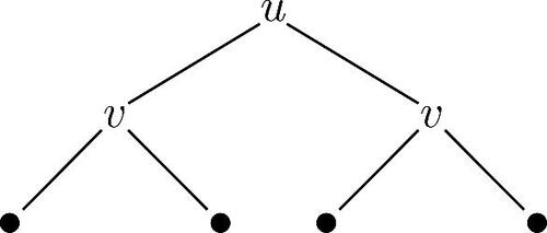
Let
be a subgraph determined by a non-terminal vertex v (and its successors) of
Fig. 2. A forbidden subtree for Theorem 3.3(iii).
Proof.
(i): By virtue of Theorem 2.1, an application of or
operation to two signed graphs such that one of them has either a repeated nonzero eigenvalue or the eigenvalue 0 with multiplicity at least 3 results in a signed graph with either a repeated eigenvalue or 0 with multiplicity at least 3. In particular, if
does not satisfy the assumptions of (i), then
has a repeated eigenvalue.
(ii): Assume for contradiction that a vertex v of has at least 3 direct successors. If v is of 0-type, then the subgraph
(determined by v) has the eigenvalue 0 with multiplicity at least 3. If v is of some of the remaining types and
has k vertices, then either k or – k is an eigenvalue with multiplicity at least 2 in
. In both cases the desired conclusion follows from the previous item.
(iii): If v is of 0-type (briefly, 0) then . If u is + (resp. –), 2 (–2) has multiplicity 2 in
, and the result follows from (i). If v is +, then in
the eigenvalue 2 has multiplicity 2 for u being 0, and 0 has multiplicity 3 for u being –, and similarly for the remaining possibility for v. Again, the result follows from (i). □
We proceed with two particular constructions. For the first one, let a -sequence determine a ∇-cograph in the following way: 1 and –1 have the same roles as in the similar sequences related to ∇-threshold graphs, while 2 (resp. –2) represents adding two non-adjacent vertices joined by positive (negative) edges to all the vertices of the already formed ∇-cograph. In particular, if a generating sequence starts with either 2 or –2, this means that in the first step we take 2 isolated vertices.
Theorem 3.4.
A -sequence generates a ∇-cograph without repeated net Laplacian eigenvalues if and only if this sequence is
Proof.
Using Theorem 2.1, we get that the sequences of (i)–(iii) generate the ∇-cographs with eigenvalues(1)
(1)
(2)
(2)
and(3)
(3) respectively. Their negations generate ∇-cographs with negated eigenvalues, which proves one implication.
Assume now that which has no repeated eigenvalues is generated by a sequence
that differs from the previous ones. In this case, every induced subgraph generated by
has no repeated nonzero eigenvalues.
For the consecutive entries bi
and
must differ in sign, as otherwise
would generate a ∇-cograph with a repeated eigenvalue (equal to i + 1 or
). Therefore, if b does not contain ±2, then b coincides with (i) or (ii), up to negation.
Assume further that b contains 2 or –2, and let , be the first occurrence of ±2 in b. According to the previous computation, the sequence
generates a ∇-cograph, say
, whose eigenvalues are up to negation given by replacing n with i in one of (1)–(3). By extending the generating sequence with
, we get
with a repeated non-zero eigenvalue. Indeed, if the spectrum of
is determined by (1), then
must differ in sign from bi
, and thus
which gives – i of multiplicity 2, and similarly if the spectrum of
is determined by the negation of (1). The remaining two possibilities ((2) and (3)) are considered in the same way.
It remains to consider the case in which . Then
, as otherwise 2 or –2 is a repeated eigenvalue of
. Thus, b starts with
or its negation. If
for
then
, as otherwise 0 has the multiplicity 2 in
. But then b coincides with (iii). If
is the first occurrence of ±2, then bi
differ in sign, and then either i or – i has multiplicity 2. This eliminates the last possibility for b and completes the proof. □
Observe that ∇-cographs generated by -sequences are obtained by removing a matching from a complete signed graph. The previous result gives those without repeated eigenvalues.
In what follows we use to denote the set of all integers from 0 to n excluding
. By
we denote the negation of the previous set. We say that a signed graph without repeated eigenvalues realizes
if its spectrum coincides with
.
The following result gives some particular constructions of ∇-cographs without repeated and without negative eigenvalues.
Theorem 3.5.
For , let
be a ∇-cograph that realizes
and
a ∇-cograph that realizes
. Then the net Laplacian eigenvalues of
are non-negative and simple if and only if i = 1 (and then
realizes
) or i = 2, j = 1 (and then
realizes
).
Proof.
The eigenvalues of are
with
and k + j removed. For
contains a repeated zero eigenvalue or a negative eigenvalue (both arise from
). For
, the spectrum of
avoids 1 and 2, which means that it must have at least one repeated eigenvalue.
For l = k, there must be i = 1; otherwise, l is a repeated eigenvalue. Then obviously realizes
.
For , there must be i = 2 (otherwise, l – 1 is a repeated eigenvalue) and also j = 1 (otherwise, l is a repeated eigenvalue). Then
realizes
. □
To get some examples we need to define the following operations. Let denote the operation
applied to an unsigned graph H. Similarly, we denote
and
. We also use
(resp.
) to denote the composition
(resp.
). We know from [Citation16] that a ∇-cograph without negative edges realizes
if and only if it is realized by the iterative procedure having one of the following forms
and it realizes if and only if it is realized by the iterative procedure having one of the following forms
These constructions are sufficient for us to establish examples for Theorem 3.5. Namely, we can take the negation of a cograph that realizes and any cograph that realizes
(here we can also take
, while for the other possibilities we refer to [Citation16]) to get a cograph that realizes
, and similarly for that realizing
.
Moreover, Theorem 3.5 enables us to give another example. We proved in Theorem 3.1 that any pair of ∇-threshold graphs differ in spectrum. The reader may recall the result in the particular case of unsigned graphs stating that every threshold graph is determined by its Laplacian spectrum (in the sense that there is no graph with the same Laplacian spectrum) [Citation10]. Naturally, we can ask whether the same holds for ∇-threshold graphs and the net Laplacian spectrum, and the answer is negative. Namely, we know from [Citation6, Citation16] that every ∇-threshold graph that realizes is generated by either
(4)
(4)
Now, using Theorem 3.5 we can construct a ∇-cograph with the same spectrum. An example is obtained by taking and the ∇-threshold graph generated by the latter sequence for i = 6. The common spectrum is
.
We further prove that every ∇-threshold graph whose eigenvalues are simple and non-negative is generated by one of the aforementioned sequences.
Theorem 3.6.
If a ∇-threshold graph generated by a
-sequence
has no repeated net Laplacian eigenvalue and has no negative net Laplacian eigenvalue, then b is one of the sequences of (4).
Proof.
We first prove that , for
. Assume that this is not true and let bi
,
, be the last occurrence of –1 in the generating sequence. In this case, by Theorem 2.1, there are at least i ones after bi
(otherwise, there is a negative eigenvalue in
). In addition, the entries of
alternately take the values of {0, 1}.
Let bj
be the ith occurrence of 1 after bi
. The ∇-threshold graph generated by
has the eigenvalue 0 of multiplicity 2, as
has the eigenvalue –1. Therefore, since
, we deduce that
has the eigenvalue 0 of multiplicity 3, and then
has a repeated eigenvalue, which is a contradiction.
Now, b1 has an arbitrary value that does not affect the corresponding signed graph, say as in (4). It is a matter of routine to verify that
implies the existence of a repeated eigenvalue in
, unless i = 1, which leads to the desired result. □
4 Computer search on connected signed graphs with 2 eigenvalues
Here is the data for computer search on connected signed graphs with at most 8 vertices and 2 eigenvalues of the net Laplacian matrix. One of these eigenvalues is 0, while the other is an integer whose absolute value does not exceed the number of vertices.
For every order n there is the complete unsigned graph with spectrum (the exponent stands for the multiplicity). For even order, there is the ∇-threshold graph
with spectrum
. The net Laplacian matrices and spectra of the remaining connected signed graphs with non-negative spectrum are given below. The negation of every signed graphs with 2 eigenvalues also has 2 eigenvalues.
5 Particular cases of 2 or 3 eigenvalues
Inspired by the previous computational results, in this section we consider some classes of signed graphs with 2 or 3 eigenvalues. In particular, we are interested in (a) regular signed graphs with 2 eigenvalues, (b) arbitrary signed graphs with 2 eigenvalues such that one of them is simple and (c) regular signed graphs with 3 eigenvalues such that 0 is a simple one.
If is net-regular with common net-degree ϱ, then we have
, which means that ν is an eigenvalue of
if and only if
is an eigenvalue of the adjacency matrix
. More interesting case arises when we drop the net-regularity and keep the regularity condition. Hence, suppose that
is a regular signed graph with vertex degree r and 2 eigenvalues: 0 and ν. Taking into account the minimal polynomial, we get
, so
. Consider now the diagonal entries of the left hand side of the last identity. We have
, and the diagonal entries of
and
are 0, while the diagonal entries of
are all equal to r. Thus, for every vertex i of
its net-degree
satisfies the quadratic equation
, which leads to the following result.
Theorem 5.1.
Let be a regular signed graph, with degree r. If
has 2 net Laplacian eigenvalues, then net-degrees of the vertices of
can take only 2 values which are solutions of the quadratic equation
, where ν is the non-zero net Laplacian eigenvalue of
.
It is well-known that, for unsigned graphs, the multiplicity of 0 in the Laplacian spectrum is equal to the number of connected components [Citation10, Citation11]. Here we have a bit different situation in which the multiplicity of 0 in the net Laplacian spectrum of is not less than the number of components [Citation14]. In other words, every component has 0 as an eigenvalue of multiplicity at least 1. Examples of connected signed graphs for which 0 is not a simple eigenvalue can be found in the previous section and also in [Citation2]. This inspires us to consider signed graphs with 2 eigenvalues such that 0 has either minimum or maximum multiplicity.
Theorem 5.2.
Let be a signed graph with 2 net Laplacian eigenvalues, 0 and ν. The following statements hold true.
If 0 is simple, then
If ν is simple, then
Proof.
(i): If the multiplicity of ν is n – 1, where n is the order of , then
is a rank one matrix with a non-zero eigenvalue
and associated eigenvector j, so
(where J denotes the all-1 matrix). Comparing the off-diagonal entries in the previous matrix identity, we deduce that ν must be equal to n or – n, and then we have
or
, which means that
is the complete unsigned graph or its negation.
(ii): If ν is simple and x is the corresponding unit eigenvector, then has the spectral decomposition
. Observe that if x has a zero entry, then the corresponding vertex is not joined to any other vertex of
. Therefore, we may suppose that there are no isolated vertices in
. Now, if xi
and xj
are the entries corresponding to the vertices i and j, then
must hold; in particular
. We also have
and
, and from
, we obtain
. This implies
, which means that
is in fact net-regular with net-degree 1 or –1. From
, we have that the trace of
is either n or – n, so ν equals n or – n, and thus
with
. Since x is orthogonal to j, n must be even, i.e.
, and the adjacency matrix
has the form
which leads to the desired result. □
We conclude the section with the following result.
Theorem 5.3.
Let be a regular signed graph with degree r, order n and 3 net Laplacian eigenvalues: simple one 0, ν and μ. Then n divides
and net-degrees are the solutions of
.
Proof.
The matrix is a rank one matrix with one nonzero eigenvalue
and the corresponding eigenvector j. Accordingly,
(5)
(5)
From the minimal polynomial , we conclude that
is an integer, which means that the off-diagonal entries of the matrix in the left-hand side of (5) are integers, and this implies that νμ is divisible by n. Considering the diagonal entries, we get that the net-degree of every vertex satisfies the quadratic equation given in the statement formulation, and we are done. □
Examples for Theorems 5.1 and 5.2 can be found in the previous section. It is not difficult to see that the ∇-threshold graph generated by (with arbitrary numbers of 1s and –1s) is an example for Theorem 5.3.
6 An application
Matrices with simple eigenvalues are required in various fields of applied mathematics. Graph theory can serve as a useful tool for their generation as well as for the analysis of their spectra. Here we emphasize an application in control theory of certain net Laplacian matrices having the mentioned spectral property.
We recall from [Citation7, Citation12] that for an binary vector b and the n × n net Laplacian matrix
of a signed graph
, the pair
is controllable if
has no eigenvector orthogonal to b. The terminology comes from the domain of control theory, and for more details we refer the reader to [Citation7, Citation8, Citation12]. In the same references one may find a more general approach concerning an arbitrary matrix and an arbitrary vector (of the appropriate size). The matrices associated with (signed) graphs have received a great deal of attention in the past; some references are [Citation5, Citation7, Citation12, Citation16, Citation14].
It follows that if has a repeated eigenvalue, then
has an eigenvector orthogonal to b for any choice of b. To see this, suppose that
and
are linearly independent eigenvectors associated with a fixed eigenvalue, and neither of them is orthogonal to b. Then the vector
is an eigenvector associated with the same eigenvalue, but also orthogonal to b. Therefore, a necessary controllability condition requires all the eigenvalues to be simple.
We consider the controllability of signed graphs of Theorems 3.4, 3.5 and of graphs obtained by some standard products. We first recall a result of [Citation15] in which the spectrum of some standard products is computed.
As in Theorem 2.1, let be a signed graph with the vertex set
and the eigenvalues
, and let
be a signed graph with the vertex set
and the eigenvalues
.
We consider the products in which the set of vertices is the Cartesian product of the sets of vertices of and
. In the Cartesian product
, the vertices (ui
, vj
) and (uk
, vl
) are adjacent if and only if ui
= uk
and
, or
and vj
= vl
. The sign of an edge coincides with the sign of the edge it arises from. In the tensor product
, the vertices (ui
, vj
) and (uk
, vl
) are adjacent if and only if
and
. The sign of an edge is the product of signs of the corresponding edges of
and
. In the strong product
, the vertices (ui
, vj
) and (uk
, vl
) are adjacent if and only if they are adjacent in any of the previous two products and the sign of an edge is determined as in the previous particular cases.
Theorem 6.1.
[Citation15, Theorem 4] For the signed graphs and
of orders n1 and n2, we have:
the net Laplacian eigenvalues of
if
if
Hence, if and
are integral, then the signed graphs constructed in the previous theorem are also integral.
In what follows we assume that the vertices of a signed graph under consideration are labeled in the order given by the corresponding operation. For example, if , then we first take the vertices of
and then those of
.
Theorem 6.2.
If is a signed graph with n vertices formed as in Theorem 3.4, then
is controllable if and only if
where c is an arbitrary binary vector of length n – 2.
Proof.
First, if the generating sequence contains just 2 entries (in this case has 2 vertices that are either non-adjacent or joined by a positive edge), then the eigenvectors of
are
and
, and so
is controllable if and only if
. Assume that the statement holds for
generated by the sequence of length n – 1. Then the eigenvectors of
are
where
are the eigenvectors of
orthogonal to j. Let
, where
is a binary vector such that
is controllable and
. Evidently, b is non-orthogonal to the eigenvectors of
which proves one implication. Conversely, if the first two entries of b are equal, then its restriction obtained by removing the last entry is non-orthogonal to all the eigenvectors of
, which contradicts our assumption on
, and the proof is complete. □
We proceed with particular ∇-cographs of Theorem 3.5. We recall from Section 2 that stands for the Euclidean inner product.
Theorem 6.3.
Let be a signed graph formed as in Theorem 3.5, so
. The pair
is controllable if and only if
where
(resp.
) is a vector of length k (l + 1) non-orthogonal to the net eigenvectors of
(
), along with
.
Proof.
Let be controllable. If
, where, say
is not as we described in the formulation of the statement, then there is an eigenvector x of
which is orthogonal to
but then
is an eigenvector of
orthogonal to b. If both
and
are as in the statement, but
, then b is orthogonal to either
or the eigenvector associated with the largest eigenvalue of
, and we are done.
Let now b be as in the statement, and let x be an eigenvector of . If x is associated with 0 or
, then
due to the particular condition on
. If x is associated with some of the remaining eigenvalues, then
, where
(resp.
) is an eigenvector of
(
) orthogonal to
(
), which yields
. □
We conclude this section by considering the signed graphs of Theorem 6.1. Since the eigenvectors of all three products considered in the mentioned theorem are the Kronecker products of the corresponding eigenvectors of and
(see [Citation15]), we conclude that if
and y are the eigenvectors of
and
, respectively, then
is an eigenvector of
.
If is a binary vector, such that length of each
is n2, then
is controllable if and only if
, for all the eigenvectors x of
and y of
. This leads to the following result.
Theorem 6.4.
Let be a signed graph formed as in Theorem 6.1, such that its net Laplacian eigenvalues are all simple, let
and
be controllable, where
, and let
. Then
is controllable.
Similar links between spectral graph theory and control theory can be found in [Citation1, Citation3, Citation5, Citation7, Citation8, Citation12, Citation14, Citation16] and references therein.
Additional information
Funding
References
- Anđelić, M., Brunetti, M., Stanić, Z. (2020). Laplacian controllability for graphs obtained by some standard products. Graphs Comb. 36: 1593–1602.
- Anđelić, M., Koledin, T., Stanić, Z. (2020). On regular signed graphs with three eigenvalues. Discuss. Math. Graph Theory 40: 405–416.
- Anđelić, M., Koledin, T., Stanić, Z. (2022). Signed graphs whose all Laplacian eigenvalues are main. Linear Multilinear Algebra.
- Corneil, D. G., Perl, Y., Stewart, L. K. (1985). A linear recognition algorithm for cographs. SIAM J. Comput. 14: 926–934.
- Cvetković, D., Rowlinson, P., Stanić, Z., Yoon, M.-G. (2011). Controllable graphs with least eigenvalue at least –2. Appl. Anal. Discrete Math. 5: 165–175.
- Fallat, S. M., Kirkland, S. J., Molitierno, J. J., Neumann, M. (2005). On graphs whose Laplacian matrices have distinct integer eigenvalues. J. Graph Theory 50: 162–174.
- Gao, H., Ji, Z., Hou, T. (2018). Equitable partitions in the controllability of undirected signed graphs. In: Proceedings of IEEE 14th International Conference on Control and Automation (ICCA). Piscataway NJ: IEEE, pp. 532–537.
- Klamka, J. (1991). Controllability of dynamical systems. Dordreht: Kluwer Academic Publishers.
- Mahadev, N. V. R., Peled, U. N. (1985). Threshold Graphs and Related Topics. New York: North-Holland.
- Merris, R. (1998). Laplacian graph eigenvectors. Linear Algebra Appl. 278: 221–236.
- Mohar, B. (1991). The Laplacian spectrum of graphs. In: Alavi, Y., Chatrand, G., Oellermann, O. R., Schwenk, A. J., eds. Graph Theory, Combinatorics, and Applications. New York: Wiley, pp. 871–898.
- Rahmani, A., Ji, M., Mesbahi, M., Egerstedt, M. (2009). Controllability of multi-agent systems from a graph theoretic perspective. SIAM J. Control Optim. 48: 162–186.
- Ramezani, F., Stanić Z. (2022). Some upper bound for the net Laplacian index of a signed graph. Bull. Iran. Math. Soc. 48: 243–250.
- Stanić, Z. (2020). Net Laplacian controllablity of joins of signed graphs. Discrete Appl. Math. 285: 197–203.
- Stanić, Z. (2020). On the spectrum of the net Laplacian matrix of a signed graph. Bull. Math. Soc. Sci. Math. Roum. 63(111): 203–211.
- Stanić, Z. (2021). Laplacian controllability for graphs with integral Laplacian spectrum. Mediterr. J. Math. 18: 35.
- Stanić, Z. (2022). Some properties of the eigenvalues of the net Laplacian matrix of a signed graph. Discuss. Math. Graph Theory 42: 893–903.
- Zaslavsky, T. (2010). Matrices in the theory of signed simple graphs. In: Acharya, B.D., Katona, G.O.H., Nešetřil, J., eds. Advances in Discrete Mathematics and Applications. Mysore: Ramanujan Mathematical Society, pp. 207–229.