Modeling the Interaction of Electrodynamic Fields to Circuit Elements

ABSTRACT

Curriculum typically addresses classical electrodynamic field theory and circuit analysis (with resistors, capacitors, and inductors) separately. As such, there exists a gap relating the two. This work provides a strong tie between these two disciplines that is useful for bridging this gap. Prior work establishes a relationship between electrodynamic fields and circuit elements, but application to circuit analysis remains ambiguous because of the path-dependent node voltages formulated. This paper develops a model resulting in path-independent node voltages that are necessary for circuit analysis techniques. The model is based on the electric field and the magnetic vector potential. Both fields have components associated with the circuit elements as well as external or excitation sources. The model is applicable for determining the coupling of excitation electrodynamic fields to transmission lines. This paper provides a rigor and collective work not found elsewhere in electrodynamic or circuit theory literature.

KEYWORDS:

• Circuit analysis
• electrodynamic field theory
• magnetic vector potential
• path-independent node voltages
• transmission line coupling

1. INTRODUCTION

Undergraduate electrical engineering curriculum typically deals with electrodynamic theory and electrical circuit analysis separately. There is a lack of literature in both disciplines strongly tying the electrodynamic theory and electrical circuit theory together. For the electrical engineering student, the curriculum includes many electrical circuit analysis courses, a general physics course, and perhaps one or two electromagnetic courses. Most general physics textbooks contain a few chapters on circuit analysis, introducing the resistor, capacitor, and inductor circuit elements.

This paper provides details of the relationship between classical electrodynamic field theory and circuit elements. The electrodynamic fields include those resulting from the voltages and currents associated with resistors, capacitors, and inductors as well as excitation fields (those originating from outside the circuit) interacting with the circuit elements.

The resistor, capacitor, and inductor elements are themselves the model incorporating the electrodynamic fields from the voltages and currents of these independent elements. This paper develops the coupling model of voltage sources in series with resistors, capacitors, and inductors as a result of the excitation electrodynamic fields.

These series voltage sources model the coupling of excitation fields into transmission line sections. This model has application for simulating the coupling of a high-altitude electromagnetic pulse (HEMP) to signal and control wires in a power substation [1].

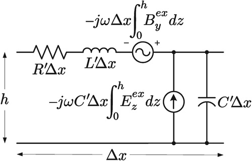
If the height of a transmission line is electrically short compared to the shortest wavelength of the excitation field [2], then a long transmission line may be broken into electrically short sections. Figure 1 shows a representative model (per unit length $\mathrm{\Delta }x$) based on the telegraph equations in prior work [3–6]. The voltage and current sources (per unit length) model the coupling of the excitation transient electromagnetic fields. The series voltage source is a function of the excitation magnetic field $B_y^{ex}$ normal to the transmission line and the parallel current source is a function of the excitation electric field $E_z^{ex}$ in the direction of the height of the transmission line. Alternative transmission line coupling models are found in other work [7–9].

Figure 1. Model of transmission line section (per unit length $\mathrm{\Delta }x$) based on prior work

Understanding the basis for the model of Figure 1 is a daunting task given the plethora of derivations in prior work based upon underlying assumptions. Various derivations for the transmission line equations incorporating excitation field coupling are found in papers on lightning [7, 10], HEMP [11, 12], or electromagnetic fields in general [13, 14]. However, there is a lack of rigor in the prior work strongly tying electrodynamic theory with circuit theory to arrive at the model of Figure 1.

The two electrodynamic fields used in the coupling models for resistors, capacitors, and inductors (and resulting transmission line model) are the electric field $⃑E$ and the magnetic vector potential $⃑A$. Since the magnetic vector potential is not unique (varies with the choice of gauge) [7, 15, 16], this paper surveys a few of the gauge possibilities. The developed transmission line model reduces to the model of Figure 1 for the one gauge identified later in this paper.

The key aspect of an electrodynamic field-to-circuit model is obtaining node voltages that are path independent. The path is any continuous route between two nodes, starting at one node and ending at the other. For circuits, the path is typically along the conductors and components and may take any branch or multiple branches. For antennas and transmission lines, the path is typically along the wire structures. However, the path can also traverse through air or other media. Node voltages that are path independent are necessary for mesh and nodal circuit analysis techniques.

Some antenna and electromagnetic theory literature contain an overview of the relationship between electrodynamic field theory and circuit elements [17–19]. However, the node voltages defined in this literature are path dependent and the literature is vague on how to use these voltages for circuit analysis. This paper clearly defines a model resulting in path-independent node voltages.

Section 2 defines the relationship between electrodynamic fields and circuit elements based on Maxwell's equations. It establishes path-independent node voltages for circuits consisting of resistors, inductors, and capacitors in the presence of excitation electrodynamic fields. Section 3 develops the model for the coupling of excitation electrodynamic fields into transmission line sections. Section 4 introduces and discusses various gauges for the path-independent node voltages.

Appendix 1 provides a terse overview of the background theory helpful for grasping the main body of this paper. Refer to the appropriate subsections in this appendix when equations and conclusions are unclear or there is a need for further explanation and understanding. Appendix 2 lists vector identities used throughout this paper.

The content of this paper is useful for undergraduate students desiring to bridge the gap between electrodynamic field and circuit theory. In addition, because of the exposure to the magnetic vector potential and various gauges, the content is applicable for students eager to advance their understanding of electrodynamic theory.

2. RELATIONSHIP BETWEEN ELECTRODYNAMIC FIELDS AND CIRCUIT ELEMENTS

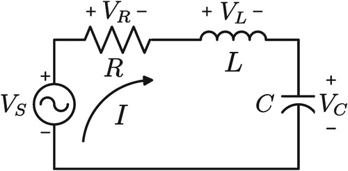
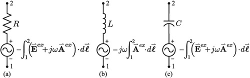
A typical circuit comprises circuit elements (resistors, inductors, and capacitors) and sinusoidal sources (voltage or current) interconnected by conductors. Kirchhoff's voltage law (KVL) states that the voltage drops of the sources and circuit elements around any given loop sums to zero [20]. The relationship between the circuital phasor current I and the circuit element phasor voltage drop is well known: (1) for a resistor R (Ω): $V_R=RI$, (2) for an inductor L (H): $V_L=\mathrm{j}\omega LI$, and (3) for a capacitor C (F): $V_C=\left(1/\mathrm{j}\omega C\right)I$ (see example circuit in Figure 2). Kirchhoff's law is applicable to electrically small circuits ( i.e. the sinusoidal current in a given loop has the same phase throughout the loop [21, 22]).

Figure 2. Example circuit loop consisting of source voltage $V_S$, resistor R, inductor L, and capacitor C

Faraday's law is the basis for KVL. Integrating both sides of (A5(A5) $Faraday\text{'}slaw:\mathrm{\nabla }\times ⃑E=-\mathrm{j}\omega ⃑B,$(A5) ) over an arbitrary surface and applying Stokes' Theorem (A47(A47) $\iint \left(\mathrm{\nabla }\times ⃑A\right)\cdot \mathrm{d}⃑\mathcal{S}=\oint ⃑A\cdot \mathrm{d}⃑\ell ,$(A47) ) to the left side yields the integral form of Faraday's law [23]: (1) $\oint ⃑E\cdot \mathrm{d}⃑\ell =-\mathrm{j}\omega \iint ⃑B\cdot \mathrm{d}⃑\mathcal{S},$(1) where $⃑E$ is the electric field (V/m), $\mathrm{d}⃑\ell$ is the differential perimeter distance element, ω is the sinusoidal radian frequency, $⃑B$ is the magnetic flux density (Wb/m²), and $\mathrm{d}⃑\mathcal{S}$ is the differential surface element. Substituting (A11(A11) $⃑B=\mathrm{\nabla }\times ⃑A,$(A11) ) into (1(1) $\oint ⃑E\cdot \mathrm{d}⃑\ell =-\mathrm{j}\omega \iint ⃑B\cdot \mathrm{d}⃑\mathcal{S},$(1) ) and applying Stokes' Theorem to the $\mathrm{\nabla }\times ⃑A$ term yields (2) $\oint ⃑E\cdot \mathrm{d}⃑\ell =-\mathrm{j}\omega \iint \left(\mathrm{\nabla }\times ⃑A\right)\cdot \mathrm{d}⃑\mathcal{S}=-\mathrm{j}\omega \oint ⃑A\cdot \mathrm{d}⃑\ell ,$(2) where ∇ is the del operator commonly used in vector calculus and $⃑A$ is the magnetic vector potential (Wb/m). Rearranging (2(2) $\oint ⃑E\cdot \mathrm{d}⃑\ell =-\mathrm{j}\omega \iint \left(\mathrm{\nabla }\times ⃑A\right)\cdot \mathrm{d}⃑\mathcal{S}=-\mathrm{j}\omega \oint ⃑A\cdot \mathrm{d}⃑\ell ,$(2) ) yields a foundational equation for KVL: (3) $-\oint \left(⃑E+\mathrm{j}\omega ⃑A\right)\cdot \mathrm{d}⃑\ell =0.$(3) The units of this equation connote the voltage around a closed loop is zero. Substituting (A13(A13) $⃑E=-\mathrm{\nabla \Phi }-\mathrm{j}\omega ⃑A,$(A13) ) into (3(3) $-\oint \left(⃑E+\mathrm{j}\omega ⃑A\right)\cdot \mathrm{d}⃑\ell =0.$(3) ) yields an equivalent equation foundational for KVL: (4) $\oint \left(\mathrm{\nabla \Phi }\right)\cdot \mathrm{d}⃑\ell =0,$(4) where Φ is the electric potential (V).

Application of Equations (3(3) $-\oint \left(⃑E+\mathrm{j}\omega ⃑A\right)\cdot \mathrm{d}⃑\ell =0.$(3) ) and (4(4) $\oint \left(\mathrm{\nabla \Phi }\right)\cdot \mathrm{d}⃑\ell =0,$(4) ) as KVL begins by defining a circuital voltage drop $V_{21}$. For a circuit segment with one node labeled 1 and another labeled 2, $V_{21}$ is the voltage of node 2 with respect to node 1 ( i.e. node 1 is the reference for the voltage of node 2). Based on (A13(A13) $⃑E=-\mathrm{\nabla \Phi }-\mathrm{j}\omega ⃑A,$(A13) ), the voltage drop $V_{21}$ is [24] (5) $\begin{array}{rl}{V}_{21}& ={\int }_1^2\left(\mathrm{\nabla \Phi }\right)\cdot \mathrm{d}⃑\ell ={\int }_1^2\frac{\mathrm{\partial \Phi }}{\mathrm{\partial }\ell }\mathrm{d}\ell ={\mathrm{\Phi }}_2-{\mathrm{\Phi }}_1\\ & =-{\int }_1^2\left(⃑E+\mathrm{j}\omega ⃑A\right)\cdot \mathrm{d}⃑\ell ,\end{array}$(5) where the integral and integral limits 1 and 2 represent the continuous path taken from node 1 to node 2 and $\mathrm{d}⃑\ell$ is in the direction along the path traversing from node 1 to node 2.

This circuital voltage drop depicts KVL since $V_{21}$ is independent of the circuit path taken. If two different paths are used for calculating $V_{21}$ of (5(5) $\begin{array}{rl}{V}_{21}& ={\int }_1^2\left(\mathrm{\nabla \Phi }\right)\cdot \mathrm{d}⃑\ell ={\int }_1^2\frac{\mathrm{\partial \Phi }}{\mathrm{\partial }\ell }\mathrm{d}\ell ={\mathrm{\Phi }}_2-{\mathrm{\Phi }}_1\\ & =-{\int }_1^2\left(⃑E+\mathrm{j}\omega ⃑A\right)\cdot \mathrm{d}⃑\ell ,\end{array}$(5) ), they form a closed loop. According to (3(3) $-\oint \left(⃑E+\mathrm{j}\omega ⃑A\right)\cdot \mathrm{d}⃑\ell =0.$(3) ) and (4(4) $\oint \left(\mathrm{\nabla \Phi }\right)\cdot \mathrm{d}⃑\ell =0,$(4) ), the two voltages are equivalent (independent of the path taken) since they must sum to zero for the closed loop consisting of both paths. Path integration with either the $\left(\mathrm{\nabla \Phi }\right)$ term or the $-(⃑E+\mathrm{j}\omega ⃑A)$ term determines the circuit voltage $V_{21}$.

For circuit analysis purposes, the electric field $⃑E$, magnetic vector potential $⃑A$, and electric potential Φ of (5(5) $\begin{array}{rl}{V}_{21}& ={\int }_1^2\left(\mathrm{\nabla \Phi }\right)\cdot \mathrm{d}⃑\ell ={\int }_1^2\frac{\mathrm{\partial \Phi }}{\mathrm{\partial }\ell }\mathrm{d}\ell ={\mathrm{\Phi }}_2-{\mathrm{\Phi }}_1\\ & =-{\int }_1^2\left(⃑E+\mathrm{j}\omega ⃑A\right)\cdot \mathrm{d}⃑\ell ,\end{array}$(5) ) consists of two parts: an excitation component ($⃑E^{-0.5ex\$ex\$}$, $⃑A^{-0.5ex\$ex\$}$, and ${\mathrm{\Phi }}^{ex}$) and a reaction component ($⃑E^{-0.5ex\$re\$}$, $⃑A^{-0.5ex\$re\$}$, and ${\mathrm{\Phi }}^{re}$). The excitation component is the electrodynamic fields originating from the voltage or current sources (or charges and currents) external to the circuit. The reaction component is the fields originating from the currents and charges in the circuit elements ( i.e. resistors, capacitors, and inductors) resulting from the sources (within the circuit) [19, 25].

The following three subsections define the relation between the circuit voltages of a resistor, inductor and capacitor and the corresponding reaction fields. The use of simple examples for the resistor, inductor, and capacitor illustrate this relationship. More complicated structures for these components ( e.g. layered capacitors) add a level of complexity and are outside the realm of this paper. The last subsection defines the relationship between the excitation fields (external to the circuit) and the voltage source (of the model) placed in series with the resistor, inductor, and capacitor. As a first approximation, the reaction field from one component is insignificant for the evaluation of the other components in the circuit and the circuit is not losing energy by radiating an electromagnetic field.

2.1. Resistor Voltage and the Reaction Electric Field

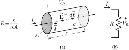
The resistor voltage $V_R$ relates to the reaction electric field: (6) $\begin{array}{rl}{V}_R& =IR=\left[\underset{\mathcal{A}}{\iint }⃑J\cdot \mathrm{d}⃑\mathcal{S}\right]\left[\frac{\ell }{\sigma \mathcal{A}}\right]\\ & =\left[-\mathcal{A}\left(⃑J\cdot {\hat{\mathbf{a}}}_{\ell }\right)\right]\left[{\int }_{V_R\left(-\right)}^{V_R\left(+\right)}\frac{1}{\sigma \mathcal{A}}\mathrm{d}\ell \right]\\ & =-{\int }_{V_R\left(-\right)}^{V_R\left(+\right)}\frac{⃑J}{\sigma }\cdot \mathrm{d}⃑\ell =-{\int }_{V_R(-)}^{V_R(+)}⃑E^{-0.5ex\$re\$}\cdot \mathrm{d}⃑\ell ,\end{array}$(6) where $R=\ell /\sigma \mathcal{A}$ is the resistance ( e.g. of the cylindrical resistor shown in Figure 3), $⃑J$ is the current density (A/m²), ℓ is the length of the resistor, σ is the conductivity (S/m) of the resistive material throughout the cylinder, $\mathcal{A}$ is the cross sectional area of the resistor, ${\hat{\mathbf{a}}}_{\ell }$ is the unit vector in the direction of $\mathrm{d}⃑\ell$, and $⃑E^{-0.5ex\$re\$}=⃑J/\sigma$ is the microscopic form of Ohm's law [26]. The limits of the line integral in (6(6) $\begin{array}{rl}{V}_R& =IR=\left[\underset{\mathcal{A}}{\iint }⃑J\cdot \mathrm{d}⃑\mathcal{S}\right]\left[\frac{\ell }{\sigma \mathcal{A}}\right]\\ & =\left[-\mathcal{A}\left(⃑J\cdot {\hat{\mathbf{a}}}_{\ell }\right)\right]\left[{\int }_{V_R\left(-\right)}^{V_R\left(+\right)}\frac{1}{\sigma \mathcal{A}}\mathrm{d}\ell \right]\\ & =-{\int }_{V_R\left(-\right)}^{V_R\left(+\right)}\frac{⃑J}{\sigma }\cdot \mathrm{d}⃑\ell =-{\int }_{V_R(-)}^{V_R(+)}⃑E^{-0.5ex\$re\$}\cdot \mathrm{d}⃑\ell ,\end{array}$(6) ), $V_R(-)$ and $V_R(+)$, are the two node ends of the resistor (similar to nodes 1 and 2 of (5(5) $\begin{array}{rl}{V}_{21}& ={\int }_1^2\left(\mathrm{\nabla \Phi }\right)\cdot \mathrm{d}⃑\ell ={\int }_1^2\frac{\mathrm{\partial \Phi }}{\mathrm{\partial }\ell }\mathrm{d}\ell ={\mathrm{\Phi }}_2-{\mathrm{\Phi }}_1\\ & =-{\int }_1^2\left(⃑E+\mathrm{j}\omega ⃑A\right)\cdot \mathrm{d}⃑\ell ,\end{array}$(5) )).

Figure 3. Resistor voltage: (a) cylindrical resistor example, (b) resistor circuit element

In the absence of an excitation field, the significance of (6(6) $\begin{array}{rl}{V}_R& =IR=\left[\underset{\mathcal{A}}{\iint }⃑J\cdot \mathrm{d}⃑\mathcal{S}\right]\left[\frac{\ell }{\sigma \mathcal{A}}\right]\\ & =\left[-\mathcal{A}\left(⃑J\cdot {\hat{\mathbf{a}}}_{\ell }\right)\right]\left[{\int }_{V_R\left(-\right)}^{V_R\left(+\right)}\frac{1}{\sigma \mathcal{A}}\mathrm{d}\ell \right]\\ & =-{\int }_{V_R\left(-\right)}^{V_R\left(+\right)}\frac{⃑J}{\sigma }\cdot \mathrm{d}⃑\ell =-{\int }_{V_R(-)}^{V_R(+)}⃑E^{-0.5ex\$re\$}\cdot \mathrm{d}⃑\ell ,\end{array}$(6) ) is that the voltage drop across the resistor is the source of the reaction electric field $⃑E^{-0.5ex\$re\$}$ and therefore the total electric field inside the resistive region. An additional perspective is the resistor symbol of Figure 3(b) models the reaction electric field by using circuit theory, thus only the effects of excitation fields (originating form charges or currents external to the circuit) need to be tacked on to the model.

The total electric field inside a resistive region is a combination of the reaction electric field and the excitation electric field: (7) $⃑E=⃑E^{-0.5ex\$re\$}+⃑E^{-0.5ex\$ex\$}.$(7) The excitation field inside the resistive material is either the transmitted field into the resistive material (for the analytical approach of an incident field from some source charges or currents having a reflective field component at the resistive material boundary and a transmitted field component into the resistive material [27]) or the summation of the incident and scattered fields (for a scattering theory approach).

For conductors ($\sigma /\epsilon \omega >100$, where ϵ is the permittivity of the material) [28], the total electric field in the conductive region is just the reaction electric field $⃑E^{-0.5ex\$re\$}$ since all the incident field is reflected or scattered, thus $⃑E=⃑J/\sigma$ [29]. For insulators ($\sigma /\epsilon \omega <1/100$) however, the total electric field in the insulator region is $⃑E=⃑J/\sigma +⃑E^{-0.5ex\$ex\$}$ since there is a portion of the incident field that is transmitted into the resistive material.

2.2. Inductor Voltage and the Reaction Magnetic Vector Potential

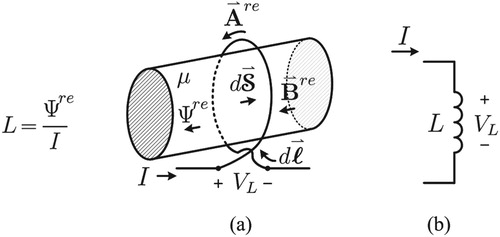
The inductor voltage $V_L$ relates to the reaction magnetic vector potential: (8) $\begin{array}{rl}{V}_L& =\mathrm{j}\omega LI=\mathrm{j}\omega {\mathrm{\Psi }}^{re}=-\mathrm{j}\omega \iint ⃑B^{-0.5ex\$re\$}\cdot \mathrm{d}⃑\mathcal{S}\\ & =-\mathrm{j}\omega {\int }_{V_L(-)}^{V_L(+)}⃑A^{-0.5ex\$re\$}\cdot \mathrm{d}⃑\ell ,\end{array}$(8) where $L={\mathrm{\Psi }}^{re}/I$ is the inductance [30] ( e.g. of the single loop inductor shown in Figure 4), the polarity of the inductance voltage $V_L$ and direction of the current I accounts for the negative sign from Lenz's law [31], and the reaction magnetic flux ${\mathrm{\Psi }}^{re}$ (Wb) equates to the surface integral of the reaction magnetic flux density $⃑B^{-0.5ex\$re\$}$ (bounded by the contour of the single loop).

Figure 4. Inductor voltage: (a) single loop inductor example, (b) inductor circuit element

The total magnetic vector potential $⃑A$ along the conductor path of an inductor is a combination of the reaction magnetic vector potential $⃑A^{-0.5ex\$re\$}$ and the excitation magnetic vector potential $⃑A^{-0.5ex\$ex\$}$. The excitation magnetic vector potential along the conductor path of an inductor is the combined incident, reflected, transmitted, or scattered magnetic vector potentials.

2.3. Capacitor Voltage and the Reaction Electric Field

Kirchhoff's current law (KCL) states that the net current exiting a node is zero [20]. KCL relates to the continuity of charge equation (A10(A10) $\mathrm{\nabla }\cdot ⃑J+\mathrm{j}\omega \rho =0$(A10) ). Integrating both sides of (A10(A10) $\mathrm{\nabla }\cdot ⃑J+\mathrm{j}\omega \rho =0$(A10) ) over an arbitrary volume and applying the divergence theorem (A48(A48) $\iiint \left(\mathrm{\nabla }\cdot ⃑A\right)\mathrm{d}\mathcal{V}=\text{∯}◯\int \int ⃑A\cdot \mathrm{d}⃑\mathcal{S},$(A48) ) to the $⃑J$ term yields (9) $\text{∯}⃑J\cdot \mathrm{d}⃑\mathcal{S}+\mathrm{j}\omega \iiint \rho \mathrm{d}\mathcal{V}=0.$(9) Applying (9(9) $\text{∯}⃑J\cdot \mathrm{d}⃑\mathcal{S}+\mathrm{j}\omega \iiint \rho \mathrm{d}\mathcal{V}=0.$(9) ) to a closed surface surrounding all the conductor branches of a circuit node yields (10) $\sum I_n+\mathrm{j}\omega q=0,$(10) where $I_n$ is the branch current exiting the nth branch and q is the charge on the node. In words, (10(10) $\sum I_n+\mathrm{j}\omega q=0,$(10) ) states that the sum of the sinusoidal branch currents exiting a node plus the sinusoidal change in charge on the node equals zero ( i.e. KCL in essence).

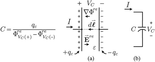
The capacitor voltage $V_C$ relates to the reaction electric field: (11) $\begin{array}{rl}{V}_C& =\frac{I}{\mathrm{j}\omega C}=\frac{I}{\mathrm{j}\omega \frac{q_c}{{\mathrm{\Phi }}_{V_C\left(+\right)}^{re}-{\mathrm{\Phi }}_{V_C\left(-\right)}^{re}}}={\mathrm{\Phi }}_{V_C\left(+\right)}^{re}-{\mathrm{\Phi }}_{V_C\left(-\right)}^{re}\\ & ={\int }_{V_C(-)}^{V_C(+)}\left(\mathrm{\nabla }{\mathrm{\Phi }}^{re}\right)\cdot \mathrm{d}⃑\ell =-{\int }_{V_C(-)}^{V_C(+)}⃑E^{-0.5ex\$re\$}\cdot \mathrm{d}⃑\ell ,\end{array}$(11) where $C=q_c/({\mathrm{\Phi }}_{V_C(+)}^{re}-{\mathrm{\Phi }}_{V_C(-)}^{re})$ is the capacitance [32] ( e.g. of the parallel plates shown in Figure 5 [33]), $q_c$ is the charge on the capacitor nodes, ${\mathrm{\Phi }}_{V_C(+)}^{re}-{\mathrm{\Phi }}_{V_C(-)}^{re}$ is the reaction electric potential difference of the capacitor nodes resulting from the node charges, and from KCL (10(10) $\sum I_n+\mathrm{j}\omega q=0,$(10) ): $I=\mathrm{j}\omega q_c$. Some electrodynamic literature do not consider the reaction magnetic vector potential term $\mathrm{j}\omega ⃑A^{-0.5ex\$re\$}$ of (5(5) $\begin{array}{rl}{V}_{21}& ={\int }_1^2\left(\mathrm{\nabla \Phi }\right)\cdot \mathrm{d}⃑\ell ={\int }_1^2\frac{\mathrm{\partial \Phi }}{\mathrm{\partial }\ell }\mathrm{d}\ell ={\mathrm{\Phi }}_2-{\mathrm{\Phi }}_1\\ & =-{\int }_1^2\left(⃑E+\mathrm{j}\omega ⃑A\right)\cdot \mathrm{d}⃑\ell ,\end{array}$(5) ) part of the capacitor but instead apply it to the inductance of the capacitor leads [34].

Figure 5. Capacitor voltage: (a) parallel plate capacitor example, (b) capacitor circuit element

Just like the resistor, the total electric field inside the dielectric material is a combination of the reaction electric field and the excitation electric field. Again, the excitation electric field inside the dielectric material is the incident electric field less any reflected or scattered electric fields.

2.4. Source Voltage and the Excitation Fields

The excitation electric field and excitation magnetic vector potential determines the source voltage $V_S$ of Figure 2: (12) $V_S=-{\int }_{V_S(-)}^{V_S(+)}(⃑E^{-0.5ex\$ex\$}+\mathrm{j}\omega ⃑A^{-0.5ex\$ex\$})\cdot \mathrm{d}⃑\ell .$(12) For most source voltages in a circuit, the physical device (such as a function generator, power supply or transformer winding) confine the excitation fields within the source region. These excitation fields do not typically couple to the resistors, inductors, and capacitors of the circuit. Likewise, the reaction fields from the circuit elements do not typically couple to the source voltage devices.

For those cases where there is an external source impacting a circuit, the model for each circuit element incorporates an additional series voltage source representing the coupling of the excitation field to the circuit element. For a physical resistor, the coupling series voltage source is (13) $V_{S_R}=-{\int }_1^2\left(⃑E^{-0.5ex\$ex\$}+\mathrm{j}\omega ⃑A^{-0.5ex\$ex\$}\right)\cdot \mathrm{d}⃑\ell .$(13) For an inductor, the coupling series voltage source is (14) $V_{S_L}=-\mathrm{j}\omega {\int }_1^2⃑A^{-0.5ex\$ex\$}\cdot \mathrm{d}⃑\ell ,$(14) and for a capacitor: (15) $V_{S_C}=-{\int }_1^2\left(⃑E^{-0.5ex\$ex\$}+\mathrm{j}\omega ⃑A^{-0.5ex\$ex\$}\right)\cdot \mathrm{d}⃑\ell .$(15) The limits 1 and 2 of (13(13) $V_{S_R}=-{\int }_1^2\left(⃑E^{-0.5ex\$ex\$}+\mathrm{j}\omega ⃑A^{-0.5ex\$ex\$}\right)\cdot \mathrm{d}⃑\ell .$(13) ), (14(14) $V_{S_L}=-\mathrm{j}\omega {\int }_1^2⃑A^{-0.5ex\$ex\$}\cdot \mathrm{d}⃑\ell ,$(14) ), and (15(15) $V_{S_C}=-{\int }_1^2\left(⃑E^{-0.5ex\$ex\$}+\mathrm{j}\omega ⃑A^{-0.5ex\$ex\$}\right)\cdot \mathrm{d}⃑\ell .$(15) ) are the node ends of the circuit elements. Figure 6 shows the modeling of the additional series voltage sources and these node ends.

Figure 6. Coupling series voltage source: (a) for a resistor, (b) for an inductor, (c) for a capacitor

Evaluating the excitation fields inside resistive, dielectric, or magnetic material (resulting from incident fields) is outside the realm of this paper. Conductors, insulators, or combinations of both are the building blocks for many wire structures such as antennas and transmission lines.

3. TRANSMISSION LINE SECTION MODEL

The model for a conductor between two nodes in the presence of an excitation field consists of the series combination of the conductor resistance, inductance, and coupling voltage source. The coupling voltage source is the combination of both (13(13) $V_{S_R}=-{\int }_1^2\left(⃑E^{-0.5ex\$ex\$}+\mathrm{j}\omega ⃑A^{-0.5ex\$ex\$}\right)\cdot \mathrm{d}⃑\ell .$(13) ) and (14(14) $V_{S_L}=-\mathrm{j}\omega {\int }_1^2⃑A^{-0.5ex\$ex\$}\cdot \mathrm{d}⃑\ell ,$(14) ) excluding the excitation electric field in the conductor. The model for an insulator between two conductor nodes in the presence of an excitation field consists of the parallel combination of insulator resistance (reciprocal of the conductance G) and capacitance (between the two conductors), both in series with a coupling voltage source. Figure 7 show these two circuit models.

Figure 7. Circuit models in the presence of a radiated excitation field for: (a) a conductor between nodes 1 & 2, (b) an insulator between conductor nodes 1 & 2

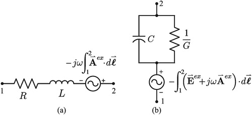
For free space, the conductance of Figure 7(b) is $G=0$. The remaining capacitance and voltage source model the charge that exists on the two conductor nodes.

As an aside, building a first-order model for a dipole antenna from two conductor segments is useful in producing a more precise model of a conductor between two nodes. The model for each arm of a dipole antenna is Figure 7(a) while the model between the two arms is similar to Figure 7(b). If the dipole antenna output nodes are shorted, it becomes a single conductor. This produces a more precise model for a conductor between two nodes ( i.e. the parallel combination of Figure 7(a) and (b)).

An important aspect of the models (depicted in Figures 6 and 7) is that the voltage of node 2 with respect to node 1 always equates to the total electric field and magnetic vector potential (reaction component plus excitation component), given any circuit currents through the model: (16) $\begin{array}{rl}{V}_{21}& =-{\int }_1^2\left(⃑E+\mathrm{j}\omega ⃑A\right)\cdot \mathrm{d}⃑\ell \\ & =-{\int }_1^2\left(⃑E^{-0.5ex\$re\$}+\mathrm{j}\omega ⃑A^{-0.5ex\$re\$}\right)\cdot \mathrm{d}⃑\ell -{\int }_1^2\left(⃑E^{-0.5ex\$ex\$}+\mathrm{j}\omega ⃑A^{-0.5ex\$ex\$}\right)\cdot \mathrm{d}⃑\ell .\end{array}$(1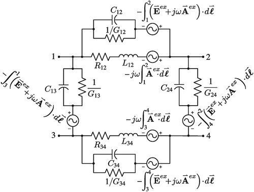6) Figure 8 shows the model for a section of a transmission line consisting of two conductors. This transmission line section model incorporates the models of Figure 7 for a conductor segment and an insulator between two conductors. Applying this model may determine the coupling from a HEMP event to a transmission line. First, use scattering theory to determine the excitation electric field and magnetic vector potential near the transmission line from the incident HEMP wave front. Second, generate the waveforms for the voltage sources of Figure 8 for each section from the HEMP excitation electric field and magnetic vector potential. And finally, use SPICE (Simulation Program with Integrated Circuit Emphasis) to solve the total circuit meshes.

Figure 8. Model of a section of transmission line (constructed with two conductors) based on Maxwell's equations and path-independent node voltages

4. GAUGE DEPENDENT NODE VOLTAGES

Electrodynamics literature uses the term gauge to define the relationship between sources (charge densities ρ and current densities $⃑J$) and the resulting potential fields (electric potential Φ and magnetic vector potential $⃑A$). The divergence of the magnetic vector potential ( i.e. $\mathrm{\nabla }\cdot ⃑A$) establishes the gauge. Students are most familiar with the Coulomb gauge ($\mathrm{\nabla }\cdot ⃑A=0$) from magnetostatic course material. However, students may not be exposed to the infinite number of gauge possibilities (refer to Section A.5 in Appendix 1 for further information on gauges).

In any given circuit, the voltage $V_{21}$ between two nodes is path independent. Path independence implies the underlying total field is conservative. By inspection of (5(5) $\begin{array}{rl}{V}_{21}& ={\int }_1^2\left(\mathrm{\nabla \Phi }\right)\cdot \mathrm{d}⃑\ell ={\int }_1^2\frac{\mathrm{\partial \Phi }}{\mathrm{\partial }\ell }\mathrm{d}\ell ={\mathrm{\Phi }}_2-{\mathrm{\Phi }}_1\\ & =-{\int }_1^2\left(⃑E+\mathrm{j}\omega ⃑A\right)\cdot \mathrm{d}⃑\ell ,\end{array}$(5) ) and (16(16) $\begin{array}{rl}{V}_{21}& =-{\int }_1^2\left(⃑E+\mathrm{j}\omega ⃑A\right)\cdot \mathrm{d}⃑\ell \\ & =-{\int }_1^2\left(⃑E^{-0.5ex\$re\$}+\mathrm{j}\omega ⃑A^{-0.5ex\$re\$}\right)\cdot \mathrm{d}⃑\ell -{\int }_1^2\left(⃑E^{-0.5ex\$ex\$}+\mathrm{j}\omega ⃑A^{-0.5ex\$ex\$}\right)\cdot \mathrm{d}⃑\ell .\end{array}$(16) ), this is the case since $⃑E+\mathrm{j}\omega ⃑A=-\mathrm{\nabla \Phi }$. However, inspection of (16(16) $\begin{array}{rl}{V}_{21}& =-{\int }_1^2\left(⃑E+\mathrm{j}\omega ⃑A\right)\cdot \mathrm{d}⃑\ell \\ & =-{\int }_1^2\left(⃑E^{-0.5ex\$re\$}+\mathrm{j}\omega ⃑A^{-0.5ex\$re\$}\right)\cdot \mathrm{d}⃑\ell -{\int }_1^2\left(⃑E^{-0.5ex\$ex\$}+\mathrm{j}\omega ⃑A^{-0.5ex\$ex\$}\right)\cdot \mathrm{d}⃑\ell .\end{array}$(16) ) reveals that this voltage is gauge dependent. Different formulas for $⃑A$ may result in different node voltages. Hence, an underlying meaning of a gauge is a corresponding 'yardstick' for determining voltages. The remainder of this section introduces three gauge possibilities.

4.1. Retarded Generalized Helmholtz Gauge

One possible gauge is the Lorenz–Neumann gauge for a Hertzian dipole source of (A31(A31) $⃑A_{\mathrm{L}-\mathrm{N}}\left(⃑r\right)=\frac{{\mu }_{\mathrm{o}}I\ell {\mathrm{e}}^{-\mathrm{j}{\beta }_{\mathrm{o}}|⃑r-⃑r{}^{\prime }|}}{4\pi |⃑r-⃑r{}^{\prime }|}{\hat{\mathbf{a}}}_I.$(A31) ). Choosing a gauge function related to the retarded version of the generalized Helmholtz gauge function [35, 36] produces an infinite number of gauges: (17) ${\chi }_k\left(⃑r\right)=\frac{\left(k-1\right){\mu }_{\mathrm{o}}I\ell {\mathrm{e}}^{-\mathrm{j}{\beta }_{\mathrm{o}}|⃑r-⃑r{}^{\prime }|}}{8\pi }{\hat{\mathbf{a}}}_I\cdot {\hat{\mathbf{a}}}_{r{r}^{\prime }},$(17) where k is an arbitrary constant ( i.e. any real number). The corresponding magnetic vector potential as a function of k is (substituting (A31(A31) $⃑A_{\mathrm{L}-\mathrm{N}}\left(⃑r\right)=\frac{{\mu }_{\mathrm{o}}I\ell {\mathrm{e}}^{-\mathrm{j}{\beta }_{\mathrm{o}}|⃑r-⃑r{}^{\prime }|}}{4\pi |⃑r-⃑r{}^{\prime }|}{\hat{\mathbf{a}}}_I.$(A31) ) and (17(17) ${\chi }_k\left(⃑r\right)=\frac{\left(k-1\right){\mu }_{\mathrm{o}}I\ell {\mathrm{e}}^{-\mathrm{j}{\beta }_{\mathrm{o}}|⃑r-⃑r{}^{\prime }|}}{8\pi }{\hat{\mathbf{a}}}_I\cdot {\hat{\mathbf{a}}}_{r{r}^{\prime }},$(17) ) into (A22(A22) $⃑A{}^{\prime }=⃑A+\mathrm{\nabla }\chi$(A22) ) and applying vector identities (A40(A40) $\mathrm{\nabla }f\left(|⃑r-⃑r{}^{\prime }|\right)=\left(\frac{\mathrm{\partial }f\left(|⃑r-⃑r{}^{\prime }|\right)}{\mathrm{\partial }|⃑r-⃑r{}^{\prime }|}\right){\hat{\mathbf{a}}}_{r{r}^{\prime }},$(A40) ) and (A42(A41) $\mathrm{\nabla }\times \left(\phi ⃑A\right)=\phi \left(\mathrm{\nabla }\times ⃑A\right)+\left(\phantom{⃑A}\mathrm{\nabla }\phi \right)\times ⃑A,$(A41) ) through (A45(A44) ${\mathrm{\nabla }}_{r-r^{\prime }}\left[\left(⃑r-⃑r{}^{\prime }\right)\cdot ⃑A\right]=⃑A,$(A44) )): (18) $\begin{array}{rl}⃑A_k\left(⃑r\right)& =⃑A_{\mathrm{L}-\mathrm{N}}\left(⃑r\right)+\mathrm{\nabla }{\chi }_k\left(⃑r\right)\\ & =\frac{{\mu }_{\mathrm{o}}I\ell {\mathrm{e}}^{-\mathrm{j}{\beta }_{\mathrm{o}}|⃑r-⃑r{}^{\prime }|}}{8\pi |⃑r-⃑r{}^{\prime }|}\left[\left(1-k\right)\left(1+\mathrm{j}{\beta }_{\mathrm{o}}|⃑r-⃑r{}^{\prime }|\right)\right.\\ & \times \left({\hat{\mathbf{a}}}_I\cdot {\hat{\mathbf{a}}}_{r{r}^{\prime }}\right){\hat{\mathbf{a}}}_{r{r}^{\prime }}\left.+\left(1+k\right){\hat{\mathbf{a}}}_I\right].\end{array}$(18) The Lorenz–Neumann electric potential is (substituting (A32(A32) $\begin{array}{rl}& \mathrm{\nabla }\cdot ⃑A_{\mathrm{L}-\mathrm{N}}\left(⃑r\right)=-\frac{{\mu }_{\mathrm{o}}I\ell {\mathrm{e}}^{-\mathrm{j}{\beta }_{\mathrm{o}}|⃑r-⃑r{}^{\prime }|}}{4\pi }\\ & \times \left(\frac{\mathrm{j}{\beta }_{\mathrm{o}}}{|⃑r-⃑r{}^{\prime }|}+\frac{1}{|⃑r-⃑r{}^{\prime }{|}^2}\right){\hat{\mathbf{a}}}_I\cdot {\hat{\mathbf{a}}}_{r{r}^{\prime }}.\end{array}$(A32) ) into (A17(A17) $\mathrm{\nabla }\cdot ⃑A=-\frac{\mathrm{j}\omega }{c^2}\mathrm{\Phi }.$(A17) )) (19) $\begin{array}{rl}{\mathrm{\Phi }}_{\mathrm{L}-\mathrm{N}}\left(⃑r\right)& =-\frac{c^2}{\mathrm{j}\omega }\mathrm{\nabla }\cdot ⃑A_{\mathrm{L}-\mathrm{N}}\left(⃑r\right)\\ & =\frac{I\ell {\mathrm{e}}^{-\mathrm{j}{\beta }_{\mathrm{o}}|⃑r-⃑r{}^{\prime }|}}{4\pi }\left(\frac{{\eta }_{\mathrm{o}}}{|⃑r-⃑r{}^{\prime }|}\right.\\ & +\left.\frac{1}{\mathrm{j}\omega {\epsilon }_{\mathrm{o}}|⃑r-⃑r{}^{\prime }{|}^2}\right){\hat{\mathbf{a}}}_I\cdot {\hat{\mathbf{a}}}_{r{r}^{\prime }},\end{array}$(19) and the gauge transformed electric potential as a function of k is (substituting (17(17) ${\chi }_k\left(⃑r\right)=\frac{\left(k-1\right){\mu }_{\mathrm{o}}I\ell {\mathrm{e}}^{-\mathrm{j}{\beta }_{\mathrm{o}}|⃑r-⃑r{}^{\prime }|}}{8\pi }{\hat{\mathbf{a}}}_I\cdot {\hat{\mathbf{a}}}_{r{r}^{\prime }},$(17) ) and (19(19) $\begin{array}{rl}{\mathrm{\Phi }}_{\mathrm{L}-\mathrm{N}}\left(⃑r\right)& =-\frac{c^2}{\mathrm{j}\omega }\mathrm{\nabla }\cdot ⃑A_{\mathrm{L}-\mathrm{N}}\left(⃑r\right)\\ & =\frac{I\ell {\mathrm{e}}^{-\mathrm{j}{\beta }_{\mathrm{o}}|⃑r-⃑r{}^{\prime }|}}{4\pi }\left(\frac{{\eta }_{\mathrm{o}}}{|⃑r-⃑r{}^{\prime }|}\right.\\ & +\left.\frac{1}{\mathrm{j}\omega {\epsilon }_{\mathrm{o}}|⃑r-⃑r{}^{\prime }{|}^2}\right){\hat{\mathbf{a}}}_I\cdot {\hat{\mathbf{a}}}_{r{r}^{\prime }},\end{array}$(19) ) into (A23(A23) ${\mathrm{\Phi }}^{\prime }=\mathrm{\Phi }-\mathrm{j}\omega \chi ,$(A23) )): (20) $\begin{array}{rl}{\mathrm{\Phi }}_k\left(⃑r\right)& ={\mathrm{\Phi }}_{\mathrm{L}-\mathrm{N}}\left(⃑r\right)-\mathrm{j}\omega {\chi }_k\left(⃑r\right)\\ & =\frac{I\ell {\mathrm{e}}^{-\mathrm{j}{\beta }_{\mathrm{o}}|⃑r-⃑r{}^{\prime }|}}{4\pi }\left(\frac{1-k}{2}\mathrm{j}\omega {\mu }_{\mathrm{o}}\right.\\ & +\left.\frac{{\eta }_{\mathrm{o}}}{|⃑r-⃑r{}^{\prime }|}+\frac{1}{\mathrm{j}\omega {\epsilon }_{\mathrm{o}}|⃑r-⃑r{}^{\prime }{|}^2}\right){\hat{\mathbf{a}}}_I\cdot {\hat{\mathbf{a}}}_{r{r}^{\prime }}.\end{array}$(20) The divergence of the retarded generalized Helmholtz magnetic vector potential (18(18) $\begin{array}{rl}⃑A_k\left(⃑r\right)& =⃑A_{\mathrm{L}-\mathrm{N}}\left(⃑r\right)+\mathrm{\nabla }{\chi }_k\left(⃑r\right)\\ & =\frac{{\mu }_{\mathrm{o}}I\ell {\mathrm{e}}^{-\mathrm{j}{\beta }_{\mathrm{o}}|⃑r-⃑r{}^{\prime }|}}{8\pi |⃑r-⃑r{}^{\prime }|}\left[\left(1-k\right)\left(1+\mathrm{j}{\beta }_{\mathrm{o}}|⃑r-⃑r{}^{\prime }|\right)\right.\\ & \times \left({\hat{\mathbf{a}}}_I\cdot {\hat{\mathbf{a}}}_{r{r}^{\prime }}\right){\hat{\mathbf{a}}}_{r{r}^{\prime }}\left.+\left(1+k\right){\hat{\mathbf{a}}}_I\right].\end{array}$(18) ) identifies the gauge (applying vector identities (A39(A39) $\mathrm{\nabla }\cdot \left(\phi ⃑A\right)=\phi \left(\mathrm{\nabla }\cdot ⃑A\right)+\left(\phantom{⃑A}\mathrm{\nabla }\phi \right)\cdot ⃑A,$(A39) ), (A40(A40) $\mathrm{\nabla }f\left(|⃑r-⃑r{}^{\prime }|\right)=\left(\frac{\mathrm{\partial }f\left(|⃑r-⃑r{}^{\prime }|\right)}{\mathrm{\partial }|⃑r-⃑r{}^{\prime }|}\right){\hat{\mathbf{a}}}_{r{r}^{\prime }},$(A40) ), (A42(A41) $\mathrm{\nabla }\times \left(\phi ⃑A\right)=\phi \left(\mathrm{\nabla }\times ⃑A\right)+\left(\phantom{⃑A}\mathrm{\nabla }\phi \right)\times ⃑A,$(A41) ) through (A45(A44) ${\mathrm{\nabla }}_{r-r^{\prime }}\left[\left(⃑r-⃑r{}^{\prime }\right)\cdot ⃑A\right]=⃑A,$(A44) ), and (A49(A49) $\mathrm{\nabla }\cdot {\hat{\mathbf{a}}}_{r{r}^{\prime }}=\frac{2}{|⃑r-⃑r{}^{\prime }|}.$(A49) )): (21) $\begin{array}{rl}& \mathrm{\nabla }\cdot ⃑A_k\left(⃑r\right)\\ & =-\frac{{\mu }_{\mathrm{o}}I\ell {\mathrm{e}}^{-\mathrm{j}{\beta }_{\mathrm{o}}|⃑r-⃑r{}^{\prime }|}}{4\pi }\left(\frac{k-1}{2}{\beta }_{\mathrm{o}}^2\right.\\ & +\left.\frac{k\mathrm{j}{\beta }_{\mathrm{o}}}{|⃑r-⃑r{}^{\prime }|}+\frac{k}{|⃑r-⃑r{}^{\prime }{|}^2}\right){\hat{\mathbf{a}}}_I\cdot {\hat{\mathbf{a}}}_{r{r}^{\prime }}.\end{array}$(21) Alternately, the divergence of $⃑A_k\left(⃑r\right)$ equates to the electric potential (combining (19(19) $\begin{array}{rl}{\mathrm{\Phi }}_{\mathrm{L}-\mathrm{N}}\left(⃑r\right)& =-\frac{c^2}{\mathrm{j}\omega }\mathrm{\nabla }\cdot ⃑A_{\mathrm{L}-\mathrm{N}}\left(⃑r\right)\\ & =\frac{I\ell {\mathrm{e}}^{-\mathrm{j}{\beta }_{\mathrm{o}}|⃑r-⃑r{}^{\prime }|}}{4\pi }\left(\frac{{\eta }_{\mathrm{o}}}{|⃑r-⃑r{}^{\prime }|}\right.\\ & +\left.\frac{1}{\mathrm{j}\omega {\epsilon }_{\mathrm{o}}|⃑r-⃑r{}^{\prime }{|}^2}\right){\hat{\mathbf{a}}}_I\cdot {\hat{\mathbf{a}}}_{r{r}^{\prime }},\end{array}$(19) ), (20(20) $\begin{array}{rl}{\mathrm{\Phi }}_k\left(⃑r\right)& ={\mathrm{\Phi }}_{\mathrm{L}-\mathrm{N}}\left(⃑r\right)-\mathrm{j}\omega {\chi }_k\left(⃑r\right)\\ & =\frac{I\ell {\mathrm{e}}^{-\mathrm{j}{\beta }_{\mathrm{o}}|⃑r-⃑r{}^{\prime }|}}{4\pi }\left(\frac{1-k}{2}\mathrm{j}\omega {\mu }_{\mathrm{o}}\right.\\ & +\left.\frac{{\eta }_{\mathrm{o}}}{|⃑r-⃑r{}^{\prime }|}+\frac{1}{\mathrm{j}\omega {\epsilon }_{\mathrm{o}}|⃑r-⃑r{}^{\prime }{|}^2}\right){\hat{\mathbf{a}}}_I\cdot {\hat{\mathbf{a}}}_{r{r}^{\prime }}.\end{array}$(20) ), and (21(21) $\begin{array}{rl}& \mathrm{\nabla }\cdot ⃑A_k\left(⃑r\right)\\ & =-\frac{{\mu }_{\mathrm{o}}I\ell {\mathrm{e}}^{-\mathrm{j}{\beta }_{\mathrm{o}}|⃑r-⃑r{}^{\prime }|}}{4\pi }\left(\frac{k-1}{2}{\beta }_{\mathrm{o}}^2\right.\\ & +\left.\frac{k\mathrm{j}{\beta }_{\mathrm{o}}}{|⃑r-⃑r{}^{\prime }|}+\frac{k}{|⃑r-⃑r{}^{\prime }{|}^2}\right){\hat{\mathbf{a}}}_I\cdot {\hat{\mathbf{a}}}_{r{r}^{\prime }}.\end{array}$(21) )): (22) $\begin{array}{rl}& \mathrm{\nabla }\cdot ⃑A_k\left(⃑r\right)\\ & =-\frac{\mathrm{j}\omega }{c^2}\left[{\mathrm{\Phi }}_k\left(⃑r\right)+\left(k-1\right){\mathrm{\Phi }}_{\mathrm{L}-\mathrm{N}}\left(⃑r\right)\right]\\ & =-k\frac{\mathrm{j}\omega }{c^2}{\mathrm{\Phi }}_{\mathrm{L}-\mathrm{N}}\left(⃑r\right)+\left(1-k\right)\frac{{\mu }_{\mathrm{o}}{\beta }_{\mathrm{o}}^{2}I\ell {\mathrm{e}}^{-\mathrm{j}{\beta }_{\mathrm{o}}|⃑r-⃑r{}^{\prime }|}}{8\pi }{\hat{\mathbf{a}}}_I\cdot {\hat{\mathbf{a}}}_{r{r}^{\prime }}.\end{array}$(22)

4.2. Retarded Kirchhoff–Weber Gauge

For quasi-statics, a unique characteristic of the Kirchhoff–Weber magnetic vector potential ($⃑A_{\mathrm{K}-\mathrm{W}}\left(⃑r\right)$ of (A30(A30) $⃑A_{\mathrm{K}-\mathrm{W}}\left(⃑r\right)=\frac{{\mu }_{\mathrm{o}}}{4\pi }\iiint \frac{\left(⃑J\left(⃑r{}^{\prime }\right)\mathrm{d}{\mathcal{V}}^{\prime }\right)\cdot {\hat{\mathbf{a}}}_{r{r}^{\prime }}}{|⃑r-⃑r{}^{\prime }|}{\hat{\mathbf{a}}}_{r{r}^{\prime }}.$(A30) )) is only having a component in the ${\hat{\mathbf{a}}}_{r{r}^{\prime }}$ direction. This is also the case, in electrodynamics, by setting $k=-1$ for the retarded generalized Helmholtz magnetic vector potential $⃑A_k\left(⃑r\right)$ of (18(18) $\begin{array}{rl}⃑A_k\left(⃑r\right)& =⃑A_{\mathrm{L}-\mathrm{N}}\left(⃑r\right)+\mathrm{\nabla }{\chi }_k\left(⃑r\right)\\ & =\frac{{\mu }_{\mathrm{o}}I\ell {\mathrm{e}}^{-\mathrm{j}{\beta }_{\mathrm{o}}|⃑r-⃑r{}^{\prime }|}}{8\pi |⃑r-⃑r{}^{\prime }|}\left[\left(1-k\right)\left(1+\mathrm{j}{\beta }_{\mathrm{o}}|⃑r-⃑r{}^{\prime }|\right)\right.\\ & \times \left({\hat{\mathbf{a}}}_I\cdot {\hat{\mathbf{a}}}_{r{r}^{\prime }}\right){\hat{\mathbf{a}}}_{r{r}^{\prime }}\left.+\left(1+k\right){\hat{\mathbf{a}}}_I\right].\end{array}$(18) ). The result is the retarded Kirchhoff–Weber magnetic vector potential: (23) $\begin{array}{rl}& ⃑A_{{\mathrm{K}-\mathrm{W}}_{cret}}\left(⃑r\right)\\ & =\frac{{\mu }_{\mathrm{o}}I\ell \left(1+\mathrm{j}{\beta }_{\mathrm{o}}|⃑r-⃑r{}^{\prime }|\right)\left({\hat{\mathbf{a}}}_I\cdot {\hat{\mathbf{a}}}_{r{r}^{\prime }}\right){\mathrm{e}}^{-\mathrm{j}{\beta }_{\mathrm{o}}|⃑r-⃑r{}^{\prime }|}}{4\pi |⃑r-⃑r{}^{\prime }|}{\hat{\mathbf{a}}}_{r{r}^{\prime }}.\end{array}$(23) The corresponding retarded Kirchhoff–Weber electric potential is (24) $\begin{array}{rl}& {\mathrm{\Phi }}_{{\mathrm{K}-\mathrm{W}}_{cret}}\left(⃑r\right)=\frac{I\ell {\mathrm{e}}^{-\mathrm{j}{\beta }_{\mathrm{o}}|⃑r-⃑r{}^{\prime }|}}{4\pi }\left(\mathrm{j}\omega {\mu }_{\mathrm{o}}+\frac{{\eta }_{\mathrm{o}}}{|⃑r-⃑r{}^{\prime }|}\right.\\ & +\left.\frac{1}{\mathrm{j}\omega {\epsilon }_{\mathrm{o}}|⃑r-⃑r{}^{\prime }{|}^2}\right){\hat{\mathbf{a}}}_I\cdot {\hat{\mathbf{a}}}_{r{r}^{\prime }}.\end{array}$(24) And, the divergence of the retarded Kirchhoff–Weber magnetic vector potential is (25) $\begin{array}{rl}& \mathrm{\nabla }\cdot ⃑A_{{\mathrm{K}-\mathrm{W}}_{cret}}\left(⃑r\right)=\frac{{\mu }_{\mathrm{o}}I\ell {\mathrm{e}}^{-\mathrm{j}{\beta }_{\mathrm{o}}|⃑r-⃑r{}^{\prime }|}}{4\pi }\\ & \times \left({\beta }_{\mathrm{o}}^2+\frac{\mathrm{j}{\beta }_{\mathrm{o}}}{|⃑r-⃑r{}^{\prime }|}+\frac{1}{|⃑r-⃑r{}^{\prime }{|}^2}\right){\hat{\mathbf{a}}}_I\cdot {\hat{\mathbf{a}}}_{r{r}^{\prime }},\end{array}$(25) or alternatively, (26) $\begin{array}{rl}\mathrm{\nabla }\cdot ⃑A_{{\mathrm{K}-\mathrm{W}}_{cret}}\left(⃑r\right)& =\frac{\mathrm{j}\omega }{c^2}\left[2{\mathrm{\Phi }}_{\mathrm{L}-\mathrm{N}}-{\mathrm{\Phi }}_{{\mathrm{K}-\mathrm{W}}_{cret}}\right]\\ & =\frac{\mathrm{j}\omega }{c^2}{\mathrm{\Phi }}_{\mathrm{L}-\mathrm{N}}+\frac{{\mu }_{\mathrm{o}}{\beta }_{\mathrm{o}}^{2}I\ell {\mathrm{e}}^{-\mathrm{j}{\beta }_{\mathrm{o}}|⃑r-⃑r{}^{\prime }|}}{4\pi }{\hat{\mathbf{a}}}_I\cdot {\hat{\mathbf{a}}}_{r{r}^{\prime }}.\end{array}$(26) The significance of the retarded Kirchhoff–Weber gauge is that differential elements of series voltages (in the differential elements of a conductor or insulator) are only in the ${\hat{\mathbf{a}}}_{r{r}^{\prime }}$ direction. This gauge is the author's preference since the series voltage may be modeled as a result of the interaction of energy carriers (bosons), similar to the bosons described in [37, 38]. The boson interaction occurs between each individual Hertzian dipole source and a particular differential element of a conductor or insulator.

4.3. Gauge for Transmission Line Coupling Model of Figure 1

Eliminating the component of the magnetic vector potential $⃑A^{-0.5ex\$ex\$}$ in the direction of the height is the first step in reducing the transmission line model of Figure 8 to the prior work model of Figure 1. Applying the right gauge transformation removes the component of $⃑A^{-0.5ex\$ex\$}$ in a given direction. For example, consider the rectangular loop of Figure 9. Using Faraday's law, the open circuit voltage of the rectangular loop from an excitation magnetic flux density $⃑B^{-0.5ex\$ex\$}$ is [39] (27) $V_{\mathit{\text{loop}}}=-\mathrm{j}\omega \iint \left(⃑B^{-0.5ex\$ex\$}\cdot {\hat{\mathbf{a}}}_{\mathcal{S}}\right)\mathrm{d}\mathcal{S},$(27) where ${\hat{\mathbf{a}}}_{\mathcal{S}}$ is the unit vector normal to the surface of the loop.

Figure 9. Rectangular loop

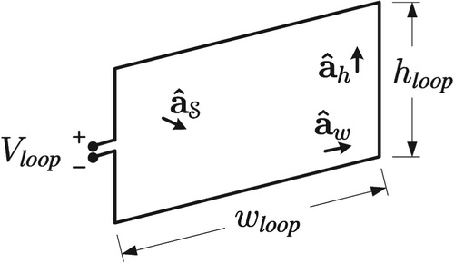
Using the conductor model of Figure 7(a), the loop voltage is also equivalent to (28) $V_{\mathit{\text{loop}}}=-\mathrm{j}\omega {\int }_{V_{\mathit{\text{loop}}}(-)}^{V_{\mathit{\text{loop}}}(+)}⃑A^{-0.5ex\$ex\$}\cdot \mathrm{d}⃑\ell .$(28) If scattering is insignificant, the excitation magnetic vector potential is nearly the incident magnetic vector potential. Assuming $⃑A^{-0.5ex\$ex\$}$ equates to the Lorenz–Neumann magnetic vector potential $⃑A_{\mathrm{L}-\mathrm{N}}\left(⃑r\right)$ of (A31(A31) $⃑A_{\mathrm{L}-\mathrm{N}}\left(⃑r\right)=\frac{{\mu }_{\mathrm{o}}I\ell {\mathrm{e}}^{-\mathrm{j}{\beta }_{\mathrm{o}}|⃑r-⃑r{}^{\prime }|}}{4\pi |⃑r-⃑r{}^{\prime }|}{\hat{\mathbf{a}}}_I.$(A31) ) (for a Hertzian dipole source), the ${\hat{\mathbf{a}}}_h$ component is removed with the gauge function: (29) ${\chi }_{\mathrm{tran}}\left(⃑r\right)=-\frac{{\mu }_{\mathrm{o}}I\ell \left({\hat{\mathbf{a}}}_I\cdot {\hat{\mathbf{a}}}_h\right)}{4\pi }\int \frac{{\mathrm{e}}^{-\mathrm{j}{\beta }_{\mathrm{o}}|⃑r-⃑r{}^{\prime }|}}{|⃑r-⃑r{}^{\prime }|}\mathrm{d}h.$(29) The transformation of the magnetic vector potential is (30) $\begin{array}{rl}⃑A_{\mathrm{tran}}\left(⃑r\right)& =⃑A_{\mathrm{L}-\mathrm{N}}\left(⃑r\right)+\mathrm{\nabla }{\chi }_{\mathrm{tran}}\left(⃑r\right)\\ & =\frac{{\mu }_{\mathrm{o}}I\ell }{4\pi }\left[\left(\left({\hat{\mathbf{a}}}_I\cdot {\hat{\mathbf{a}}}_w\right)\frac{{\mathrm{e}}^{-\mathrm{j}{\beta }_{\mathrm{o}}|⃑r-⃑r{}^{\prime }|}}{|⃑r-⃑r{}^{\prime }|}\right.\right.\\ & -\left.\left({\hat{\mathbf{a}}}_I\cdot {\hat{\mathbf{a}}}_h\right)\frac{\mathrm{\partial }}{\mathrm{\partial }w}\int \frac{{\mathrm{e}}^{-\mathrm{j}{\beta }_{\mathrm{o}}|⃑r-⃑r{}^{\prime }|}}{|⃑r-⃑r{}^{\prime }|}\mathrm{d}h\right){\hat{\mathbf{a}}}_w\\ & +\left(\left({\hat{\mathbf{a}}}_I\cdot {\hat{\mathbf{a}}}_{\mathcal{S}}\right)\frac{{\mathrm{e}}^{-\mathrm{j}{\beta }_{\mathrm{o}}|⃑r-⃑r{}^{\prime }|}}{|⃑r-⃑r{}^{\prime }|}-\left({\hat{\mathbf{a}}}_I\cdot {\hat{\mathbf{a}}}_h\right)\right.\\ & \times \left.\left.\frac{\mathrm{\partial }}{\mathrm{\partial }\mathcal{S}}\int \frac{{\mathrm{e}}^{-\mathrm{j}{\beta }_{\mathrm{o}}|⃑r-⃑r{}^{\prime }|}}{|⃑r-⃑r{}^{\prime }|}\mathrm{d}h\right){\hat{\mathbf{a}}}_{\mathcal{S}}\right],\end{array}$(30) where (31) $9.811.9⃑A_{\mathrm{L}-\mathrm{N}}\left(⃑r\right)=\left(⃑A_{\mathrm{L}-\mathrm{N}}\right(⃑r)\cdot {\hat{\mathbf{a}}}_w){\hat{\mathbf{a}}}_w+\left(⃑A_{\mathrm{L}-\mathrm{N}}\right(⃑r)\cdot {\hat{\mathbf{a}}}_h){\hat{\mathbf{a}}}_h+\cdots .$(31)

For this gauge, the voltage sources from the magnetic vector potential only appear on the upper and lower horizontal portions of the loop antenna of Figure 9. This may be interpreted as the induced voltage in the loop is only from the upper and lower sections. However, there exists a different gauge where the induced voltage in the loop is only from the left and right vertical sections. As an aside, with the infinite number of gauge possibilities, there are an infinite number of segment voltage combinations, all giving the same total loop voltage. Showing that all the possible gauges give the same loop voltage, either analytically or with model simulations, is outside the scope of this paper.

With the ${\hat{\mathbf{a}}}_h$ component for $⃑A_{\mathrm{tran}}\left(⃑r\right)$ null, the model of the transmission line section of Figure 8 reduces to the model of Figure 10 by (a) ignoring the second-order effects related to the $C_{12}$, $G_{12}$, $C_{34}$, $G_{34}$, $G_{13}$, and $G_{24}$ elements, (b) moving the bottom segment elements and voltage source and combining them with the top segment, and (c) converting the line integral of the magnetic vector potential of (28(28) $V_{\mathit{\text{loop}}}=-\mathrm{j}\omega {\int }_{V_{\mathit{\text{loop}}}(-)}^{V_{\mathit{\text{loop}}}(+)}⃑A^{-0.5ex\$ex\$}\cdot \mathrm{d}⃑\ell .$(28) ) to the surface integral of magnetic flux density of (27(27) $V_{\mathit{\text{loop}}}=-\mathrm{j}\omega \iint \left(⃑B^{-0.5ex\$ex\$}\cdot {\hat{\mathbf{a}}}_{\mathcal{S}}\right)\mathrm{d}\mathcal{S},$(27) ).

Figure 10. Model of transmission line section similar to prior work

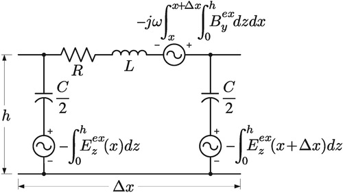
Figure 10 is the pi representation of a per unit transmission line model. This model is equivalent to the prior work model of Figure 1 by (a) lumping the capacitance on the left with the transmission section to the left and lumping the capacitance of the transmission section to the right with the capacitance on the right, (b) converting the voltage source in series with the capacitance to a Norton equivalent current source in parallel with the capacitance, and (c) assuming the magnetic flux density is constant in the x direction for the transmission line section, thus reducing the integration in the x direction to $\mathrm{\Delta }x$ (this is only valid if $\mathrm{\Delta }x$ is much less than h).

A similar gauge function (replacing ${\hat{\mathbf{a}}}_h$ with ${\hat{\mathbf{a}}}_w$ in (29(29) ${\chi }_{\mathrm{tran}}\left(⃑r\right)=-\frac{{\mu }_{\mathrm{o}}I\ell \left({\hat{\mathbf{a}}}_I\cdot {\hat{\mathbf{a}}}_h\right)}{4\pi }\int \frac{{\mathrm{e}}^{-\mathrm{j}{\beta }_{\mathrm{o}}|⃑r-⃑r{}^{\prime }|}}{|⃑r-⃑r{}^{\prime }|}\mathrm{d}h.$(29) )) eliminates the voltage source in series with the top segment of Figure 10, leaving the remaining voltage source as a function of both $⃑E^{-0.5ex\$ex\$}$ and $⃑B^{-0.5ex\$ex\$}$. Therefore, the author challenges the seemingly arbitrary choice of the gauge function (29(29) ${\chi }_{\mathrm{tran}}\left(⃑r\right)=-\frac{{\mu }_{\mathrm{o}}I\ell \left({\hat{\mathbf{a}}}_I\cdot {\hat{\mathbf{a}}}_h\right)}{4\pi }\int \frac{{\mathrm{e}}^{-\mathrm{j}{\beta }_{\mathrm{o}}|⃑r-⃑r{}^{\prime }|}}{|⃑r-⃑r{}^{\prime }|}\mathrm{d}h.$(29) ) for mesh analysis of the transmission line sections.

The models of Figures 8 and 10 may be used to determine the voltages at both ends of a transmission line for various terminating impedances at the ends and various locations for the source of an excitation field. Validating that these voltages are the same, for any of the infinite gauges in addition to empirical results, is a significant undertaking and outside the scope of this paper.

5. CONCLUSIONS

The modeling of the interaction of electrodynamic fields to circuit elements involves the electric field $⃑E$ and the magnetic vector potential $⃑A$. The resistor, inductor, and capacitor circuit elements are themselves the model accounting for the reaction electrodynamic field component from the voltages and currents associated with these circuit elements. In other words, the circuit elements are the model capturing the reaction electrodynamic field component. Voltage sources (in series with the circuit elements) model the coupling of the excitation electrodynamic field component.

The field-to-circuit model of this paper strongly ties electrodynamic theory and electrical circuit theory together. The model is useful in circuit analysis techniques (involving excitation fields coupling to circuit elements) since node voltages are path independent. Using this model captures the coupling of excitation fields to wire structures such as antennas and transmission lines.

The model developed in this paper for coupling an excitation electrodynamic field into a transmission line section is based on Maxwell's equations and path-independent node voltages. It may be useful for simulating the coupling of HEMP and other excitation electrodynamic fields into a transmission line using SPICE. However, before relying on the simulation outcomes, the model should be validated with empirical results.

Even though the resistor, inductor, and capacitor models established in this paper are for very simple structures, they are still only first-order approximation models. The resistor and inductor models don't include the capacitance associated with the element node ends and the resistor and capacitor models don't include the partial inductance of the element leads. In addition, actual capacitor, inductor, and some resistor elements are more complicated than the simple structures given as examples in this paper. Modeling complex element structures and second- and third-order effects are outside the scope of the paper.

Although the field-to-circuit model produces path-independent node voltages, the node voltages are gauge dependent. The retarded Kirchhoff–Weber gauge is the author's preference since the excitation voltage sources (in series with the resistor, inductor, capacitor, conductor, and insulator circuit elements) may be modeled as a result of the interaction of bosons exchanging between the Hertzian dipole excitation sources and the circuit elements.

The field-to-circuit model of this paper provides the foundation for further investigation of various magnetic vector potential gauges as well as the coupling of excitation fields into simply wire structures such as antennas and transmission lines.

ACKNOWLEDGEMENTS

The author would like to thank Schweitzer Engineering Laboratories, Inc., Pullman, WA for their support in the continued education of their employees.

ORCID

Timothy M. Minteer http://orcid.org/0000-0002-1502-6444

Additional information

Notes on contributors

Timothy M. Minteer

Timothy M Minteer received the BS degree in electrical engineering from Montana State University, Bozeman, MT, in 1985, and the MS and PhD degrees in electrical engineering from Washington State University, Pullman,WA, in 2008 and 2013, respectively. He is an analog and digital circuit design engineer with Schweitzer Engineering Laboratories, Inc. (SEL), Pullman,WA since 1995 and is currently a Fellow Engineer in the Power Systems Department of Research & Development. Prior to joining SEL, he was with the Montana Power Company (MPC) as a protective relay engineer since 1991 and Tetragenics (a subsidiary ofMPC) as an analog and digital circuit design engineer (1985–1991). Mr Minteer is a registered Professional Engineer in the state of Washington. His main interests are the application of electrodynamic theory and principles to design, analyze, and improve electronic circuits and systems. Mr Minteer holds seven US patents and is the author of nine publications relating to electrodynamic theory and application.

Notes

1 Electrodynamic publications typically define the wave equations with $+{\beta }_{\mathrm{o}}^2$ in place of $-(\mathrm{j}\omega /c{)}^2$. However, this paper uses $-(\mathrm{j}\omega /c{)}^2$ to emphasize the double time derivative.

APPENDIX 1. BACKGROUND THEORY

This appendix provides a terse overview of the background theory helpful for grasping the main body of this paper. The subsections are stand-alone and introduce symbols and terms used consistently throughout the paper (these may differ slightly from the symbols and terms found in the references).

A.1. Phasor Representation of Sinusoidal Electromagnetic Fields

This paper considers vector fields (i.e. $⃑A$) as phasor vector fields: (A1) $⃑A=A_m{\mathrm{e}}^{\mathrm{j}{\theta }_{\mathrm{A}}}{\hat{\mathbf{a}}}_{\mathrm{A}},$(A1) where ${\hat{\mathbf{a}}}_{\mathrm{A}}$ is a unit vector in the direction of $⃑A$ and $A_m{\mathrm{e}}^{\mathrm{j}{\theta }_{\mathrm{A}}}$ is a sinusoidal phasor in the usual sense [40]: (A2) $\begin{array}{rl}{A}_m{\mathrm{e}}^{\mathrm{j}{\theta }_{\mathrm{A}}}& =A_m\cos {\theta }_{\mathrm{A}}+\mathrm{j}{A}_m\sin {\theta }_{\mathrm{A}}\\ & ⟺\mathrm{Re}\left\{A_m{\mathrm{e}}^{\mathrm{j}\left(\omega t+{\theta }_{\mathrm{A}}\right)}\right\}=A_m\cos \left(\omega t+{\theta }_{\mathrm{A}}\right),\end{array}$(A2) where $A_m$ is the phasor magnitude (peak of the sinusoidal field), ${\theta }_{\mathrm{A}}$ is the phasor angle (phase of the sinusoidal field), and ω is the sinusoidal radian frequency. Recall that the phasor vector field $⃑A$ implies ${\mathrm{e}}^{\mathrm{j}\omega t}$, thus $\mathrm{\partial }⃑A/\mathrm{\partial }t=\mathrm{j}\omega ⃑A$. In addition, scalar fields ( i.e. Φ) are considered phasor scalar fields: $\mathrm{\Phi }={\mathrm{\Phi }}_m{\mathrm{e}}^{\mathrm{j}{\theta }_{\mathrm{\Phi }}}$.

A.2. Maxwell's Equations for Phasor Fields

Maxwell's equations are the basis for classical electrodynamics [41]. Heaviside combined Maxwell's thirteen general electromagnetic field equations [42] into the four vector based equations universally known as Maxwell's equations [43]. The four Maxwell–Heaviside equations for sinusoidal phasor electromagnetic fields [44] in SI (MKS) units are (A3) $Gauss\text{'}slawformagnetism:\mathrm{\nabla }\cdot ⃑B=0,$(A3) where $⃑B$ is the magnetic flux density (Wb/m²). (A4) $Gauss\text{'}slawforelectricity:\mathrm{\nabla }\cdot ⃑D=\rho ,$(A4) where $⃑D$ is the electric flux density (C/m²) and ρ is the charge density (C/m³). (A5) $Faraday\text{'}slaw:\mathrm{\nabla }\times ⃑E=-\mathrm{j}\omega ⃑B,$(A5) where $⃑E$ is the electric field (V/m). (A6) $Amp\stackrel{`}{e}re-Maxwell\text{'}slaw:\mathrm{\nabla }\times ⃑H=\mathrm{j}\omega ⃑D+⃑J,$(A6) where $⃑H$ is the magnetic field (A/m) and $⃑J$ is the current density (A/m²).

The constitutive equations for free space are [45] (A7) $⃑D={\epsilon }_{\mathrm{o}}⃑E,$(A7) where ${\epsilon }_{\mathrm{o}}=8.854\times {10}^{-12}$ (F/m) is the permittivity of free space and (A8) $⃑B={\mu }_{\mathrm{o}}⃑H,$(A8) where ${\mu }_{\mathrm{o}}=4\pi \times {10}^{-7}$ (H/m) is the permeability of free space.

The continuity of charge is derived by taking the divergence of both sides of (A6(A6) $Amp\stackrel{`}{e}re-Maxwell\text{'}slaw:\mathrm{\nabla }\times ⃑H=\mathrm{j}\omega ⃑D+⃑J,$(A6) ): (A9) $\mathrm{\nabla }\cdot \left(\mathrm{\nabla }\times ⃑H\right)=\mathrm{\nabla }\cdot ⃑J+\mathrm{\nabla }\cdot \left(\mathrm{j}\omega ⃑D\right)=\mathrm{\nabla }\cdot ⃑J+\mathrm{j}\omega \left(\mathrm{\nabla }\cdot ⃑D\right).$(A9) Applying vector identity (A36(A1) $⃑A=A_m{\mathrm{e}}^{\mathrm{j}{\theta }_{\mathrm{A}}}{\hat{\mathbf{a}}}_{\mathrm{A}},$(A1) ) and substituting (A4(A4) $Gauss\text{'}slawforelectricity:\mathrm{\nabla }\cdot ⃑D=\rho ,$(A4) ) into (A9(A9) $\mathrm{\nabla }\cdot \left(\mathrm{\nabla }\times ⃑H\right)=\mathrm{\nabla }\cdot ⃑J+\mathrm{\nabla }\cdot \left(\mathrm{j}\omega ⃑D\right)=\mathrm{\nabla }\cdot ⃑J+\mathrm{j}\omega \left(\mathrm{\nabla }\cdot ⃑D\right).$(A9) ) yields the continuity of charge equation [46]: (A10) $\mathrm{\nabla }\cdot ⃑J+\mathrm{j}\omega \rho =0$(A10)

A.3. Magnetic Vector Potential and Electric Potential

Electrodynamic curriculum typically introduces the magnetic vector potential for simplifying electromagnetic field solutions. The general consensus is that the physical fields are the electric and magnetic fields while the potential fields are mathematical (non-physical). Applying vector identity (A36(A1) $⃑A=A_m{\mathrm{e}}^{\mathrm{j}{\theta }_{\mathrm{A}}}{\hat{\mathbf{a}}}_{\mathrm{A}},$(A1) ) to Gauss's law for magnetism (A3(A3) $Gauss\text{'}slawformagnetism:\mathrm{\nabla }\cdot ⃑B=0,$(A3) ) yields (A11) $⃑B=\mathrm{\nabla }\times ⃑A,$(A11) where $⃑A$ is an arbitrary vector field whose curl is $⃑B$. By definition, $⃑A$ is the magnetic vector potential (Wb/m) [47].

Substituting (A11(A11) $⃑B=\mathrm{\nabla }\times ⃑A,$(A11) ) into Faraday's law (A5(A5) $Faraday\text{'}slaw:\mathrm{\nabla }\times ⃑E=-\mathrm{j}\omega ⃑B,$(A5) ) yields (A12) $\mathrm{\nabla }\times \left(-⃑E-\mathrm{j}\omega ⃑A\right)=0.$(A12) Applying vector identity (A37(A2) $\begin{array}{rl}{A}_m{\mathrm{e}}^{\mathrm{j}{\theta }_{\mathrm{A}}}& =A_m\cos {\theta }_{\mathrm{A}}+\mathrm{j}{A}_m\sin {\theta }_{\mathrm{A}}\\ & ⟺\mathrm{Re}\left\{A_m{\mathrm{e}}^{\mathrm{j}\left(\omega t+{\theta }_{\mathrm{A}}\right)}\right\}=A_m\cos \left(\omega t+{\theta }_{\mathrm{A}}\right),\end{array}$(A2) ) to (A12(A12) $\mathrm{\nabla }\times \left(-⃑E-\mathrm{j}\omega ⃑A\right)=0.$(A12) ) yields (A13) $⃑E=-\mathrm{\nabla \Phi }-\mathrm{j}\omega ⃑A,$(A13) where Φ is an arbitrary scalar field whose gradient is $-⃑E-\mathrm{j}\omega ⃑A$. By definition, Φ is the electric potential (V) [47].

Electrodynamic publications typically attribute the potentials $⃑A$ and Φ as mathematical artifacts of vector identities (A36(A1) $⃑A=A_m{\mathrm{e}}^{\mathrm{j}{\theta }_{\mathrm{A}}}{\hat{\mathbf{a}}}_{\mathrm{A}},$(A1) ) and (A37(A2) $\begin{array}{rl}{A}_m{\mathrm{e}}^{\mathrm{j}{\theta }_{\mathrm{A}}}& =A_m\cos {\theta }_{\mathrm{A}}+\mathrm{j}{A}_m\sin {\theta }_{\mathrm{A}}\\ & ⟺\mathrm{Re}\left\{A_m{\mathrm{e}}^{\mathrm{j}\left(\omega t+{\theta }_{\mathrm{A}}\right)}\right\}=A_m\cos \left(\omega t+{\theta }_{\mathrm{A}}\right),\end{array}$(A2) ) applied to Maxwell's equations. Any solutions for $⃑A$ and Φ which meet (A12(A12) $\mathrm{\nabla }\times \left(-⃑E-\mathrm{j}\omega ⃑A\right)=0.$(A12) ) and (A13(A13) $⃑E=-\mathrm{\nabla \Phi }-\mathrm{j}\omega ⃑A,$(A13) ) are valid for deriving the $⃑E$ and $⃑B$ fields.

The electric field $⃑E$ for a source free region ($⃑J=0$) may be calculated solely from the magnetic vector potential (combining Ampère–Maxwell's law (A6(A6) $Amp\stackrel{`}{e}re-Maxwell\text{'}slaw:\mathrm{\nabla }\times ⃑H=\mathrm{j}\omega ⃑D+⃑J,$(A6) ) with (A11(A11) $⃑B=\mathrm{\nabla }\times ⃑A,$(A11) ), solving $⃑E$ for a source free region, and applying vector identity (A38(A3) $Gauss\text{'}slawformagnetism:\mathrm{\nabla }\cdot ⃑B=0,$(A3) )): (A14) $⃑E=\frac{c^2}{\mathrm{j}\omega }\mathrm{\nabla }\times \mathrm{\nabla }\times ⃑A=\frac{c^2}{\mathrm{j}\omega }\left[\mathrm{\nabla }\left(\mathrm{\nabla }\cdot ⃑A\right)-{\mathrm{\nabla }}^2⃑A\right],$(A14) where $c=2.998\times {10}^8$ (m/s) is the speed of light in free space [48] ($c^2=1/\left({\mu }_{\mathrm{o}}{\epsilon }_{\mathrm{o}}\right)$).

A.4. Potential Wave Equations Solution

Electrodynamic publications typically define the electromagnetic wave equations in terms of the electric and magnetic fields. However, wave equations for the potentials may also be developed. Combining Ampère–Maxwell's law (A6(A6) $Amp\stackrel{`}{e}re-Maxwell\text{'}slaw:\mathrm{\nabla }\times ⃑H=\mathrm{j}\omega ⃑D+⃑J,$(A6) ) with (A11(A11) $⃑B=\mathrm{\nabla }\times ⃑A,$(A11) ), applying vector identity (A38(A3) $Gauss\text{'}slawformagnetism:\mathrm{\nabla }\cdot ⃑B=0,$(A3) ), and substituting (A13(A13) $⃑E=-\mathrm{\nabla \Phi }-\mathrm{j}\omega ⃑A,$(A13) ) yields the magnetic vector potential wave equation¹ [49]: (A15) $\left[{\mathrm{\nabla }}^2-{\left(\frac{\mathrm{j}\omega }{c}\right)}^2\right]⃑A={\mu }_{\mathrm{o}}⃑J+\mathrm{\nabla }\left(\mathrm{\nabla }\cdot ⃑A+\frac{\mathrm{j}\omega }{c^2}\mathrm{\Phi }\right).$(A15) Substituting (A13(A13) $⃑E=-\mathrm{\nabla \Phi }-\mathrm{j}\omega ⃑A,$(A13) ) into Gauss's law for electricity (A4(A4) $Gauss\text{'}slawforelectricity:\mathrm{\nabla }\cdot ⃑D=\rho ,$(A4) ) and rearranging yields the electric potential wave equation [49]: (A16) $\left[{\mathrm{\nabla }}^2-{\left(\frac{\mathrm{j}\omega }{c}\right)}^2\right]\mathrm{\Phi }=-\frac{\rho }{{\epsilon }_{\mathrm{o}}}-\mathrm{j}\omega \left(\mathrm{\nabla }\cdot ⃑A+\frac{\mathrm{j}\omega }{c^2}\mathrm{\Phi }\right).$(A16) The Lorenz condition simplifies and decouples the potential wave equations [50]: (A17) $\mathrm{\nabla }\cdot ⃑A=-\frac{\mathrm{j}\omega }{c^2}\mathrm{\Phi }.$(A17) Applying the Lorenz condition (A17(A17) $\mathrm{\nabla }\cdot ⃑A=-\frac{\mathrm{j}\omega }{c^2}\mathrm{\Phi }.$(A17) ) to (A15(A15) $\left[{\mathrm{\nabla }}^2-{\left(\frac{\mathrm{j}\omega }{c}\right)}^2\right]⃑A={\mu }_{\mathrm{o}}⃑J+\mathrm{\nabla }\left(\mathrm{\nabla }\cdot ⃑A+\frac{\mathrm{j}\omega }{c^2}\mathrm{\Phi }\right).$(A15) ) and (A16(A16) $\left[{\mathrm{\nabla }}^2-{\left(\frac{\mathrm{j}\omega }{c}\right)}^2\right]\mathrm{\Phi }=-\frac{\rho }{{\epsilon }_{\mathrm{o}}}-\mathrm{j}\omega \left(\mathrm{\nabla }\cdot ⃑A+\frac{\mathrm{j}\omega }{c^2}\mathrm{\Phi }\right).$(A16) ) yields the uncoupled potential wave equations [50]: (A18) $\left[{\mathrm{\nabla }}^2-{\left(\frac{\mathrm{j}\omega }{c}\right)}^2\right]⃑A={\mu }_{\mathrm{o}}⃑J$(A18) and (A19) $\left[{\mathrm{\nabla }}^2-{\left(\frac{\mathrm{j}\omega }{c}\right)}^2\right]\mathrm{\Phi }=-\frac{\rho }{{\epsilon }_{\mathrm{o}}}.$(A19) Lorenz formulated the retarded Neumann potentials as a solution to the uncoupled potential wave equations [51]. In phasor notation, the Lorenz–Neumann magnetic vector potential and electric potential are [52] (A20) $⃑A_{\mathrm{L}-\mathrm{N}}\left(⃑r\right)=\frac{{\mu }_{\mathrm{o}}}{4\pi }\iiint \frac{⃑J\left(⃑r{}^{\prime }\right){\mathrm{e}}^{-\mathrm{j}{\beta }_{\mathrm{o}}|⃑r-⃑r{}^{\prime }|}}{|⃑r-⃑r{}^{\prime }|}\mathrm{d}{\mathcal{V}}^{\prime }$(A20) and (A21) ${\mathrm{\Phi }}_{\mathrm{L}-\mathrm{N}}\left(⃑r\right)=\frac{1}{4\pi {\epsilon }_{\mathrm{o}}}\iiint \frac{\rho \left(⃑r{}^{\prime }\right){\mathrm{e}}^{-\mathrm{j}{\beta }_{\mathrm{o}}|⃑r-⃑r{}^{\prime }|}}{|⃑r-⃑r{}^{\prime }|}\mathrm{d}{\mathcal{V}}^{\prime },$(A21) where $⃑r$ is the potential field location, $⃑r{}^{\prime }$ is the current or charge density location, ${\beta }_{\mathrm{o}}=\omega /c$, and $d{\mathcal{V}}^{\prime }$ is the differential element of volume (m³). By applying the continuity of charge equation (A10(A10) $\mathrm{\nabla }\cdot ⃑J+\mathrm{j}\omega \rho =0$(A10) ), with the ${\mathrm{\nabla }}^{\prime }$ operator instead of ∇, (A20(A20) $⃑A_{\mathrm{L}-\mathrm{N}}\left(⃑r\right)=\frac{{\mu }_{\mathrm{o}}}{4\pi }\iiint \frac{⃑J\left(⃑r{}^{\prime }\right){\mathrm{e}}^{-\mathrm{j}{\beta }_{\mathrm{o}}|⃑r-⃑r{}^{\prime }|}}{|⃑r-⃑r{}^{\prime }|}\mathrm{d}{\mathcal{V}}^{\prime }$(A20) ) and (A21(A21) ${\mathrm{\Phi }}_{\mathrm{L}-\mathrm{N}}\left(⃑r\right)=\frac{1}{4\pi {\epsilon }_{\mathrm{o}}}\iiint \frac{\rho \left(⃑r{}^{\prime }\right){\mathrm{e}}^{-\mathrm{j}{\beta }_{\mathrm{o}}|⃑r-⃑r{}^{\prime }|}}{|⃑r-⃑r{}^{\prime }|}\mathrm{d}{\mathcal{V}}^{\prime },$(A21) ) are related by the Lorenz condition (A17(A17) $\mathrm{\nabla }\cdot ⃑A=-\frac{\mathrm{j}\omega }{c^2}\mathrm{\Phi }.$(A17) ) [53].

A.5. Gauge Transformation

There are an infinite number of other solutions to the potential wave equations (A15(A15) $\left[{\mathrm{\nabla }}^2-{\left(\frac{\mathrm{j}\omega }{c}\right)}^2\right]⃑A={\mu }_{\mathrm{o}}⃑J+\mathrm{\nabla }\left(\mathrm{\nabla }\cdot ⃑A+\frac{\mathrm{j}\omega }{c^2}\mathrm{\Phi }\right).$(A15) ) and (A16(A16) $\left[{\mathrm{\nabla }}^2-{\left(\frac{\mathrm{j}\omega }{c}\right)}^2\right]\mathrm{\Phi }=-\frac{\rho }{{\epsilon }_{\mathrm{o}}}-\mathrm{j}\omega \left(\mathrm{\nabla }\cdot ⃑A+\frac{\mathrm{j}\omega }{c^2}\mathrm{\Phi }\right).$(A16) ). Given a magnetic vector potential $⃑A$ and electric potential Φ solution, a new magnetic vector potential $⃑A{}^{\prime }$ and electric potential ${\mathrm{\Phi }}^{\prime }$ solution is obtained by using the gauge transformation equations [16]: (A22) $⃑A{}^{\prime }=⃑A+\mathrm{\nabla }\chi$(A22) and (A23) ${\mathrm{\Phi }}^{\prime }=\mathrm{\Phi }-\mathrm{j}\omega \chi ,$(A23) where χ is referred to as the gauge function and is an arbitrary scalar field.

A gauge transformation does not affect the magnetic flux density $⃑B$ (using (A11(A11) $⃑B=\mathrm{\nabla }\times ⃑A,$(A11) ), (A22(A22) $⃑A{}^{\prime }=⃑A+\mathrm{\nabla }\chi$(A22) ), and vector identity (A37(A2) $\begin{array}{rl}{A}_m{\mathrm{e}}^{\mathrm{j}{\theta }_{\mathrm{A}}}& =A_m\cos {\theta }_{\mathrm{A}}+\mathrm{j}{A}_m\sin {\theta }_{\mathrm{A}}\\ & ⟺\mathrm{Re}\left\{A_m{\mathrm{e}}^{\mathrm{j}\left(\omega t+{\theta }_{\mathrm{A}}\right)}\right\}=A_m\cos \left(\omega t+{\theta }_{\mathrm{A}}\right),\end{array}$(A2) )): (A24) $⃑B{}^{\prime }=\mathrm{\nabla }\times ⃑A{}^{\prime }=\mathrm{\nabla }\times \left(⃑A+\mathrm{\nabla }\chi \right)=\mathrm{\nabla }\times ⃑A=⃑B,$(A24) nor the electric field $⃑E$ (using (A13(A13) $⃑E=-\mathrm{\nabla \Phi }-\mathrm{j}\omega ⃑A,$(A13) ), (A22(A22) $⃑A{}^{\prime }=⃑A+\mathrm{\nabla }\chi$(A22) ), and (A23(A23) ${\mathrm{\Phi }}^{\prime }=\mathrm{\Phi }-\mathrm{j}\omega \chi ,$(A23) )): (A25) $\begin{array}{rl}⃑E{}^{\prime }& =-\mathrm{\nabla }{\mathrm{\Phi }}^{\prime }-\mathrm{j}\omega ⃑A{}^{\prime }=-\mathrm{\nabla }\left(\mathrm{\Phi }-\mathrm{j}\omega \chi \right)-\mathrm{j}\omega \left(⃑A+\mathrm{\nabla }\chi \right)\\ & =-\mathrm{\nabla \Phi }-\mathrm{j}\omega ⃑A=⃑E.\end{array}$(A25) Although not necessary for a gauge transformation, any gauge function ${\chi }_{\mathrm{L}}$ that meets the following criteria maintains the Lorenz condition (A17(A17) $\mathrm{\nabla }\cdot ⃑A=-\frac{\mathrm{j}\omega }{c^2}\mathrm{\Phi }.$(A17) ) provided the original potentials met the condition [49]: (A26) $\left[{\mathrm{\nabla }}^2-{\left(\frac{\mathrm{j}\omega }{c}\right)}^2\right]{\chi }_{\mathrm{L}}=0.$(A26) If a particular gauge meets the Lorenz condition (A17(A17) $\mathrm{\nabla }\cdot ⃑A=-\frac{\mathrm{j}\omega }{c^2}\mathrm{\Phi }.$(A17) ) then the relationship between the magnetic vector potential and electric field for a source free region (A14(A14) $⃑E=\frac{c^2}{\mathrm{j}\omega }\mathrm{\nabla }\times \mathrm{\nabla }\times ⃑A=\frac{c^2}{\mathrm{j}\omega }\left[\mathrm{\nabla }\left(\mathrm{\nabla }\cdot ⃑A\right)-{\mathrm{\nabla }}^2⃑A\right],$(A14) ) reduces to [54] (A27) $⃑E=-\mathrm{j}\omega ⃑A+\frac{c^2}{\mathrm{j}\omega }\mathrm{\nabla }\left(\mathrm{\nabla }\cdot ⃑A\right).$(A27) The divergence of $⃑A$ identifies the gauge or gauge set. For magnetostatics, the closed circuit Coulomb gauge ($\mathrm{\nabla }\cdot ⃑A=0$) has an infinite subset of gauges for the differential magnetic vector potential [37]: (A28) $\mathrm{\nabla }\cdot \mathrm{d}⃑A\left(⃑r\right)=-\frac{{\mu }_{\mathrm{o}}k}{4\pi |⃑r-⃑r{}^{\prime }{|}^2}\left(⃑J\left(⃑r{}^{\prime }\right)\mathrm{d}{\mathcal{V}}^{\prime }\right)\cdot {\hat{\mathbf{a}}}_{r{r}^{\prime }},$(A28) where $\mathrm{d}⃑A\left(⃑r\right)$ is the differential magnetic vector potential at location $⃑r$, k is an arbitrary constant ( i.e. any real number), and ${\hat{\mathbf{a}}}_{r{r}^{\prime }}$ is the unit vector from $⃑r{}^{\prime }$ to $⃑r$: ${\hat{\mathbf{a}}}_{r{r}^{\prime }}=(⃑r-⃑r{}^{\prime })/|⃑r-⃑r{}^{\prime }|$.

For quasi-statics, in addition to the gauge identity of (A28(A28) $\mathrm{\nabla }\cdot \mathrm{d}⃑A\left(⃑r\right)=-\frac{{\mu }_{\mathrm{o}}k}{4\pi |⃑r-⃑r{}^{\prime }{|}^2}\left(⃑J\left(⃑r{}^{\prime }\right)\mathrm{d}{\mathcal{V}}^{\prime }\right)\cdot {\hat{\mathbf{a}}}_{r{r}^{\prime }},$(A28) ), the divergence of the magnetic vector potential equates to the derivative of the electric potential [35,55]: (A29) $\mathrm{\nabla }\cdot \mathrm{d}⃑A\left(⃑r\right)=-\frac{\mathrm{j}\omega k}{c^2}\mathrm{d}\mathrm{\Phi }\left(⃑r\right),$(A29) where $\mathrm{d}\mathrm{\Phi }\left(⃑r\right)$ is the instantaneous differential electric potential (the integrand of (A21(A21) ${\mathrm{\Phi }}_{\mathrm{L}-\mathrm{N}}\left(⃑r\right)=\frac{1}{4\pi {\epsilon }_{\mathrm{o}}}\iiint \frac{\rho \left(⃑r{}^{\prime }\right){\mathrm{e}}^{-\mathrm{j}{\beta }_{\mathrm{o}}|⃑r-⃑r{}^{\prime }|}}{|⃑r-⃑r{}^{\prime }|}\mathrm{d}{\mathcal{V}}^{\prime },$(A21) ) without the retarded term ${\mathrm{e}}^{-\mathrm{j}{\beta }_{\mathrm{o}}|⃑r-⃑r{}^{\prime }|}$). If $k=1$, the gauge meets the Lorenz condition (A17(A17) $\mathrm{\nabla }\cdot ⃑A=-\frac{\mathrm{j}\omega }{c^2}\mathrm{\Phi }.$(A17) ) and the instantaneous magnetic vector potential (Neumann gauge) is (A20(A20) $⃑A_{\mathrm{L}-\mathrm{N}}\left(⃑r\right)=\frac{{\mu }_{\mathrm{o}}}{4\pi }\iiint \frac{⃑J\left(⃑r{}^{\prime }\right){\mathrm{e}}^{-\mathrm{j}{\beta }_{\mathrm{o}}|⃑r-⃑r{}^{\prime }|}}{|⃑r-⃑r{}^{\prime }|}\mathrm{d}{\mathcal{V}}^{\prime }$(A20) ) without the retarded term. If $k=-1$, the instantaneous magnetic vector potential is the Kirchhoff–Weber gauge [35]: (A30) $⃑A_{\mathrm{K}-\mathrm{W}}\left(⃑r\right)=\frac{{\mu }_{\mathrm{o}}}{4\pi }\iiint \frac{\left(⃑J\left(⃑r{}^{\prime }\right)\mathrm{d}{\mathcal{V}}^{\prime }\right)\cdot {\hat{\mathbf{a}}}_{r{r}^{\prime }}}{|⃑r-⃑r{}^{\prime }|}{\hat{\mathbf{a}}}_{r{r}^{\prime }}.$(A30)

A.6. Hertzian Dipole Source

The Hertzian dipole consists of a sinusoidal current I uniform over a differentially short length ℓ. The Hertzian dipole is a fundamental model building block since any current distribution source may be divided into the sum (perhaps infinite) of Hertzian dipoles. For a Hertzian dipole: $⃑J\mathrm{d}\mathcal{V}=I\ell {\hat{\mathbf{a}}}_I$, where ${\hat{\mathbf{a}}}_I$ is the unit vector in the direction of the dipole current. The Lorenz–Neumann magnetic vector potential for a Hertzian dipole at location $⃑r{}^{\prime }$ is (A31) $⃑A_{\mathrm{L}-\mathrm{N}}\left(⃑r\right)=\frac{{\mu }_{\mathrm{o}}I\ell {\mathrm{e}}^{-\mathrm{j}{\beta }_{\mathrm{o}}|⃑r-⃑r{}^{\prime }|}}{4\pi |⃑r-⃑r{}^{\prime }|}{\hat{\mathbf{a}}}_I.$(A31) The Lorenz–Neumann magnetic vector potential is only in the direction ${\hat{\mathbf{a}}}_I$ of the current.

The main body of this paper defines the magnetic vector potential in terms of the Herzian dipole to avoid having to write out the triple integral of (A20(A20) $⃑A_{\mathrm{L}-\mathrm{N}}\left(⃑r\right)=\frac{{\mu }_{\mathrm{o}}}{4\pi }\iiint \frac{⃑J\left(⃑r{}^{\prime }\right){\mathrm{e}}^{-\mathrm{j}{\beta }_{\mathrm{o}}|⃑r-⃑r{}^{\prime }|}}{|⃑r-⃑r{}^{\prime }|}\mathrm{d}{\mathcal{V}}^{\prime }$(A20) ) or the differential magnetic vector notation of (A28(A28) $\mathrm{\nabla }\cdot \mathrm{d}⃑A\left(⃑r\right)=-\frac{{\mu }_{\mathrm{o}}k}{4\pi |⃑r-⃑r{}^{\prime }{|}^2}\left(⃑J\left(⃑r{}^{\prime }\right)\mathrm{d}{\mathcal{V}}^{\prime }\right)\cdot {\hat{\mathbf{a}}}_{r{r}^{\prime }},$(A28) ). In addition to meeting the Lorenz condition (A17(A17) $\mathrm{\nabla }\cdot ⃑A=-\frac{\mathrm{j}\omega }{c^2}\mathrm{\Phi }.$(A17) ), the divergence of the magnetic vector potential (A31(A31) $⃑A_{\mathrm{L}-\mathrm{N}}\left(⃑r\right)=\frac{{\mu }_{\mathrm{o}}I\ell {\mathrm{e}}^{-\mathrm{j}{\beta }_{\mathrm{o}}|⃑r-⃑r{}^{\prime }|}}{4\pi |⃑r-⃑r{}^{\prime }|}{\hat{\mathbf{a}}}_I.$(A31) ) is (applying vector identities (A39(A4) $Gauss\text{'}slawforelectricity:\mathrm{\nabla }\cdot ⃑D=\rho ,$(A4) ), (A40(A5) $Faraday\text{'}slaw:\mathrm{\nabla }\times ⃑E=-\mathrm{j}\omega ⃑B,$(A5) ), and $\mathrm{\nabla }\cdot {\hat{\mathbf{a}}}_I=0$): (A32) $\begin{array}{rl}& \mathrm{\nabla }\cdot ⃑A_{\mathrm{L}-\mathrm{N}}\left(⃑r\right)=-\frac{{\mu }_{\mathrm{o}}I\ell {\mathrm{e}}^{-\mathrm{j}{\beta }_{\mathrm{o}}|⃑r-⃑r{}^{\prime }|}}{4\pi }\\ & \times \left(\frac{\mathrm{j}{\beta }_{\mathrm{o}}}{|⃑r-⃑r{}^{\prime }|}+\frac{1}{|⃑r-⃑r{}^{\prime }{|}^2}\right){\hat{\mathbf{a}}}_I\cdot {\hat{\mathbf{a}}}_{r{r}^{\prime }}.\end{array}$(A32) The magnetic flux density at location $⃑r$ from a Hertzian dipole at location $⃑r{}^{\prime }$ is (substituting (A31(A31) $⃑A_{\mathrm{L}-\mathrm{N}}\left(⃑r\right)=\frac{{\mu }_{\mathrm{o}}I\ell {\mathrm{e}}^{-\mathrm{j}{\beta }_{\mathrm{o}}|⃑r-⃑r{}^{\prime }|}}{4\pi |⃑r-⃑r{}^{\prime }|}{\hat{\mathbf{a}}}_I.$(A31) ) into (A11(A11) $⃑B=\mathrm{\nabla }\times ⃑A,$(A11) ) and applying vector identities (A40(A5) $Faraday\text{'}slaw:\mathrm{\nabla }\times ⃑E=-\mathrm{j}\omega ⃑B,$(A5) ), (A41(A6) $Amp\stackrel{`}{e}re-Maxwell\text{'}slaw:\mathrm{\nabla }\times ⃑H=\mathrm{j}\omega ⃑D+⃑J,$(A6) ), and $\mathrm{\nabla }\times {\hat{\mathbf{a}}}_I=0$) [56]: (A33) $\begin{array}{rl}& ⃑B_{\mathit{\text{Hertzian}}}\left(⃑r\right)=\mathrm{\nabla }\times ⃑A_{\mathrm{L}-\mathrm{N}}\left(⃑r\right)=\frac{{\mu }_{\mathrm{o}}I\ell {\mathrm{e}}^{-\mathrm{j}{\beta }_{\mathrm{o}}|⃑r-⃑r{}^{\prime }|}}{4\pi }\\ & \times \left(\frac{\mathrm{j}{\beta }_{\mathrm{o}}}{|⃑r-⃑r{}^{\prime }|}+\frac{1}{|⃑r-⃑r{}^{\prime }{|}^2}\right){\hat{\mathbf{a}}}_I\times {\hat{\mathbf{a}}}_{r{r}^{\prime }}.\end{array}$(A33) The electric field at location $⃑r$ from a Hertzian dipole at location $⃑r{}^{\prime }$ is (substituting (A32(A32) $\begin{array}{rl}& \mathrm{\nabla }\cdot ⃑A_{\mathrm{L}-\mathrm{N}}\left(⃑r\right)=-\frac{{\mu }_{\mathrm{o}}I\ell {\mathrm{e}}^{-\mathrm{j}{\beta }_{\mathrm{o}}|⃑r-⃑r{}^{\prime }|}}{4\pi }\\ & \times \left(\frac{\mathrm{j}{\beta }_{\mathrm{o}}}{|⃑r-⃑r{}^{\prime }|}+\frac{1}{|⃑r-⃑r{}^{\prime }{|}^2}\right){\hat{\mathbf{a}}}_I\cdot {\hat{\mathbf{a}}}_{r{r}^{\prime }}.\end{array}$(A32) ) into (A27(A27) $⃑E=-\mathrm{j}\omega ⃑A+\frac{c^2}{\mathrm{j}\omega }\mathrm{\nabla }\left(\mathrm{\nabla }\cdot ⃑A\right).$(A27) ) and applying vector identities (A40(A5) $Faraday\text{'}slaw:\mathrm{\nabla }\times ⃑E=-\mathrm{j}\omega ⃑B,$(A5) ) and (A42(A7) $⃑D={\epsilon }_{\mathrm{o}}⃑E,$(A7) ) through (A45(A10) $\mathrm{\nabla }\cdot ⃑J+\mathrm{j}\omega \rho =0$(A10) )): (A34) $\begin{array}{rl}& ⃑E_{\mathit{\text{Hertzian}}}\left(⃑r\right)=-\mathrm{j}\omega ⃑A_{\mathrm{L}-\mathrm{N}}\left(⃑r\right)+\frac{c^2}{\mathrm{j}\omega }\mathrm{\nabla }\left(\mathrm{\nabla }\cdot ⃑A_{\mathrm{L}-\mathrm{N}}\left(⃑r\right)\right)\\ & =\frac{I\ell {\mathrm{e}}^{-\mathrm{j}{\beta }_{\mathrm{o}}|⃑r-⃑r{}^{\prime }|}}{4\pi }\left[\left(\frac{\mathrm{j}\omega {\mu }_{\mathrm{o}}}{|⃑r-⃑r{}^{\prime }|}+\frac{3{\eta }_{\mathrm{o}}}{|⃑r-⃑r{}^{\prime }{|}^2}+\frac{3}{\mathrm{j}\omega {\epsilon }_{\mathrm{o}}|⃑r-⃑r{}^{\prime }{|}^3}\right)\right.\\ & \times \left({\hat{\mathbf{a}}}_I\cdot {\hat{\mathbf{a}}}_{r{r}^{\prime }}\right){\hat{\mathbf{a}}}_{r{r}^{\prime }}\\ & \left.-\left(\frac{\mathrm{j}\omega {\mu }_{\mathrm{o}}}{|⃑r-⃑r{}^{\prime }|}+\frac{{\eta }_{\mathrm{o}}}{|⃑r-⃑r{}^{\prime }{|}^2}+\frac{1}{\mathrm{j}\omega {\epsilon }_{\mathrm{o}}|⃑r-⃑r{}^{\prime }{|}^3}\right){\hat{\mathbf{a}}}_I\right],\end{array}$(A34) where ${\eta }_{\mathrm{o}}=\sqrt{{\mu }_{\mathrm{o}}/{\epsilon }_{\mathrm{o}}}$ is the intrinsic impedance of free space.

The Hertzian dipole electric field (A34(A34) $\begin{array}{rl}& ⃑E_{\mathit{\text{Hertzian}}}\left(⃑r\right)=-\mathrm{j}\omega ⃑A_{\mathrm{L}-\mathrm{N}}\left(⃑r\right)+\frac{c^2}{\mathrm{j}\omega }\mathrm{\nabla }\left(\mathrm{\nabla }\cdot ⃑A_{\mathrm{L}-\mathrm{N}}\left(⃑r\right)\right)\\ & =\frac{I\ell {\mathrm{e}}^{-\mathrm{j}{\beta }_{\mathrm{o}}|⃑r-⃑r{}^{\prime }|}}{4\pi }\left[\left(\frac{\mathrm{j}\omega {\mu }_{\mathrm{o}}}{|⃑r-⃑r{}^{\prime }|}+\frac{3{\eta }_{\mathrm{o}}}{|⃑r-⃑r{}^{\prime }{|}^2}+\frac{3}{\mathrm{j}\omega {\epsilon }_{\mathrm{o}}|⃑r-⃑r{}^{\prime }{|}^3}\right)\right.\\ & \times \left({\hat{\mathbf{a}}}_I\cdot {\hat{\mathbf{a}}}_{r{r}^{\prime }}\right){\hat{\mathbf{a}}}_{r{r}^{\prime }}\\ & \left.-\left(\frac{\mathrm{j}\omega {\mu }_{\mathrm{o}}}{|⃑r-⃑r{}^{\prime }|}+\frac{{\eta }_{\mathrm{o}}}{|⃑r-⃑r{}^{\prime }{|}^2}+\frac{1}{\mathrm{j}\omega {\epsilon }_{\mathrm{o}}|⃑r-⃑r{}^{\prime }{|}^3}\right){\hat{\mathbf{a}}}_I\right],\end{array}$(A34) ) has components in the direction of ${\hat{\mathbf{a}}}_{r{r}^{\prime }}$ and ${\hat{\mathbf{a}}}_I$. One of the components is proportional to the derivative of the dipole current ($\mathrm{j}\omega$ in the numerator), a second component is proportional to the current, and a third component is proportional to the integral of the dipole current ($\mathrm{j}\omega$ in the denominator). Electrodynamic publications typically rearrange the Hertzian dipole electric field to have components in the direction of ${\hat{\mathbf{a}}}_{r{r}^{\prime }}$ and normal to that direction (applying vector identity (A46(A11) $⃑B=\mathrm{\nabla }\times ⃑A,$(A11) )) [57]: (A35) $\begin{array}{rl}& ⃑E_{\mathit{\text{Hertzian}}}\left(⃑r\right)=\frac{I\ell {\mathrm{e}}^{-\mathrm{j}{\beta }_{\mathrm{o}}|⃑r-⃑r{}^{\prime }|}}{4\pi }\\ & \times \left[\left(\frac{\mathrm{j}\omega {\mu }_{\mathrm{o}}}{|⃑r-⃑r{}^{\prime }|}+\frac{{\eta }_{\mathrm{o}}}{|⃑r-⃑r{}^{\prime }{|}^2}+\frac{1}{\mathrm{j}\omega {\epsilon }_{\mathrm{o}}|⃑r-⃑r{}^{\prime }{|}^3}\right)\right.\\ & \times \left({\hat{\mathbf{a}}}_I\times {\hat{\mathbf{a}}}_{r{r}^{\prime }}\right)\times {\hat{\mathbf{a}}}_{r{r}^{\prime }}\\ & \left.+2\left(\frac{{\eta }_{\mathrm{o}}}{|⃑r-⃑r{}^{\prime }{|}^2}+\frac{1}{\mathrm{j}\omega {\epsilon }_{\mathrm{o}}|⃑r-⃑r{}^{\prime }{|}^3}\right)\left({\hat{\mathbf{a}}}_I\cdot {\hat{\mathbf{a}}}_{r{r}^{\prime }}\right){\hat{\mathbf{a}}}_{r{r}^{\prime }}\right].\end{array}$(A35)

Appendix 2. VECTOR IDENTITIES

(A36) $\mathrm{\nabla }\cdot \left(\mathrm{\nabla }\times ⃑A\right)=0,$(A36) (A37) $\mathrm{\nabla }\times \left(\phantom{⃑A}\mathrm{\nabla }\phi \right)=0,$(A37) (A38) $\mathrm{\nabla }\times \left(\mathrm{\nabla }\times ⃑A\right)=\mathrm{\nabla }\left(\mathrm{\nabla }\cdot ⃑A\right)-{\mathrm{\nabla }}^2⃑A,$(A38) (A39) $\mathrm{\nabla }\cdot \left(\phi ⃑A\right)=\phi \left(\mathrm{\nabla }\cdot ⃑A\right)+\left(\phantom{⃑A}\mathrm{\nabla }\phi \right)\cdot ⃑A,$(A39) (A40) $\mathrm{\nabla }f\left(|⃑r-⃑r{}^{\prime }|\right)=\left(\frac{\mathrm{\partial }f\left(|⃑r-⃑r{}^{\prime }|\right)}{\mathrm{\partial }|⃑r-⃑r{}^{\prime }|}\right){\hat{\mathbf{a}}}_{r{r}^{\prime }},$(A40) (A41) $\mathrm{\nabla }\times \left(\phi ⃑A\right)=\phi \left(\mathrm{\nabla }\times ⃑A\right)+\left(\phantom{⃑A}\mathrm{\nabla }\phi \right)\times ⃑A,$(A41) (A42) $\mathrm{\nabla }\left(\phi \psi \right)=\phi \mathrm{\nabla }\psi +\psi \mathrm{\nabla }\phi ,$(A42) (A43) $\mathrm{\nabla }\left(⃑A\cdot ⃑B\right)={\mathrm{\nabla }}_{\mathrm{A}}\left(⃑A\cdot ⃑B\right)+{\mathrm{\nabla }}_{\mathrm{B}}\left(⃑A\cdot ⃑B\right),$(A43) (A44) ${\mathrm{\nabla }}_{r-r^{\prime }}\left[\left(⃑r-⃑r{}^{\prime }\right)\cdot ⃑A\right]=⃑A,$(A44) (A45) ${\mathrm{\nabla }}_{{\mathrm{a}}_I}\left[{\hat{\mathbf{a}}}_I\cdot ⃑A\right]=0,$(A45) (A46) $⃑A=\left({\hat{\mathbf{a}}}_{\mathrm{B}}\cdot ⃑A\right){\hat{\mathbf{a}}}_{\mathrm{B}}+\left({\hat{\mathbf{a}}}_{\mathrm{B}}\times ⃑A\right)\times {\hat{\mathbf{a}}}_{\mathrm{B}}.$(A46) Stokes' Theorem [58]: (A47) $\iint \left(\mathrm{\nabla }\times ⃑A\right)\cdot \mathrm{d}⃑\mathcal{S}=\oint ⃑A\cdot \mathrm{d}⃑\ell ,$(A47) where in accordance with the right-hand rule, when the extended thumb of the right hand is in the general direction of the differential surface element $\mathrm{d}⃑\mathcal{S}$, then the gripped fingers are in the general direction of the differential perimeter distance element $\mathrm{d}⃑\ell$.

Divergence theorem: (A48) $\iiint \left(\mathrm{\nabla }\cdot ⃑A\right)\mathrm{d}\mathcal{V}=\text{∯}◯\int \int ⃑A\cdot \mathrm{d}⃑\mathcal{S},$(A48) (A49) $\mathrm{\nabla }\cdot {\hat{\mathbf{a}}}_{r{r}^{\prime }}=\frac{2}{|⃑r-⃑r{}^{\prime }|}.$(A49)

References

- T. Minteer, T. Mooney, S. Artz, and D. E. Whitehead, “Understanding design, installation and testing methods that promote substation IED resiliency for high-altitude electromagnetic pulse events,” in 2017 70th Annual Conference for Protective Relay Engineers (CPRE), Apr. 2017.
- C. R. Paul, Introduction to Electromagnetic Compatibility. New York: John Wiley & Sons Ltd, 2006, p. 14.
- F. Rachidi, “A review of field-to-transmission line coupling models with special emphasis to lightning-induced voltages on overhead lines,” IEEE Trans. Electromagn. Compatibility, Vol. 54, no. 4, pp. 898–911, Feb. 2012.
- F. M. Tesche, M. V. Ianoz, and T. Karlsson, EMC Analysis Methods and Computational Models. New York: 1997. p. 329–32.
- F. Rachidi, “Formulation of the field-to-transmission line coupling equations in terms of magnetic excitation field,” IEEE Trans. Electromagn. Compatibility, Vol. 35, no. 3, pp. 404–7, Aug. 1993.
- C. R. Paul, “Frequency response of multiconductor transmission lines illuminated by an electromagnetic field,” IEEE Trans. Electromagn. Compatibility, Vol. EMC-18, no. 4, pp. 183–90, Nov. 1976.
- V. Cooray, F. Rachidi, and M. Rubinstein, “Formulation of the field-to-transmission line coupling equations in terms of scalar and vector potentials,” IEEE Trans. Electromagn. Compatibility, Vol. tbd, no. tbd, pp. 1–6, Mar. 2017.
- M. Ianoz, B. I. C. Nicoara, and W. A. Radasky, “Modeling of an EMP conducted environment,” IEEE Trans. Electromagn. Compatibility, Vol. 38, no. 3, pp. 400–13, Aug. 1996.
- M. Rubinstein, A. Y. Tzeng, M. A. Uman, P. J. Medelius, and E. M. Thomson, “An experimental test of a theory of lightning-induced voltages on an overhead wire,” IEEE Trans. Electromagn. Compatibility, Vol. 31, no. 4, pp. 376–83, Nov. 1989.
- M. Paolone, F. Rachidi, A. Borghetti, C. A. Nucci, M. Rubinstein, V. A. Rakov, and M. A. Uman, “Lightning electromagnetic field coupling to overhead lines: Theory, numerical simulations, and experimental validation,” IEEE Trans. Electromagn. Compatibility, Vol. 51, no. 3, pp. 532–47, Aug. 2009.
- H. Xie, Y. Li, H. Qiao, and J. Wang, “Empirical formula of effective coupling length for transmission lines illuminated by E1 HEMP,” IEEE Trans. Electromagn. Compatibility, Vol. 58, no. 2, pp. 581–7, Apr. 2016.
- H. Xie, T. Du, M. Zhang, Y. Li, H. Qiao, J. Yang, Y. Shi, and J. Wang, “Theoretical and experimental study of effective coupling length for transmission lines illuminated by HEMP,” IEEE Trans. Electromagn. Compatibility, Vol. 57, no. 6, pp. 1529–38, Dec. 2015.
- S. Tkatchenko, F. Rachidi, and M. Ianoz, “High-frequency electromagnetic field coupling to long terminated lines,” IEEE Trans. Electromagn. Compatibility, Vol. 43, no. 2, pp. 117–29, May 2001.
- C. A. Nucci and F. Rachidi, “On the contribution of the electromagnetic field components in field-to-transmission line interaction,” IEEE Trans. Electromagn. Compatibility, Vol. 37, no. 4, pp. 505–8, Nov. 1995.
- C. Ni, Z. Zhao, and X. Cui, “Partial inductance of conductor segments with Coulomb gauge in quasi-static field,” IEEE Trans. Electromagn. Compatibility, Vol. 59, no. 4, pp. 1125–32, Mar. 2017.
- J. D. Jackson, “From Lorenz to Coulomb and other explicit gauge transformations,” <DIFadd>Am. J. Phys., Vol. 70, no. 9, pp. 917–28, Sep. 2002.
- J. D. Kraus, Electromagnetics. New York: McGraw-Hill Book Company, Inc., 1953, p. 331–43.
- S. Ramo and J. R. Whinnery, Fields and Waves in Modern Radio. New York: John Wiley & Sons, Inc., 1953, pp. 207–29.
- J. R. Carson, “Electromagnetic theory and the foundations of electric circuit theory,” Bell Syst. Tech. J., Vol. 6, pp. 1–17, Jan. 1927.
- G. R. Kirchhoff, “Ueber den durchgang eines elektrischen stromes durch eine ebene, insbesondere durch eine kreisformige,” Ann. Phys. Chem., Vol. 64, no. 4, pp. 497–514, 1845, English translation of title: “About the electric current running through a plane, especially through a circular form”, KVL: top line of p. 502, KCL: under 1) near bottom of p. 513.
- D. J. Griffiths, Introduction to Electrodynamics. Englewood Cliffs NJ: Prentice-Hall, 1981, p. 308.
- F. W. Grover, Inductance Calculations. Mineola, NY: Dover Publications, Inc., 1973, pp. 2–3.
- O. D. Jefimenko, Electricity and Magnetism. Star City, WV: Electret Scientific Company, 1989, pp. 497–8.
- S. Ramo and J. R. Whinnery, Fields and Waves in Modern Radio. New York: John Wiley & Sons, Inc., 1953, p. 203.
- S. Ramo and J. R. Whinnery, Fields and Waves in Modern Radio. New York: John Wiley & Sons, Inc., 1953, p. 210.
- O. D. Jefimenko, Electricity and Magnetism. Star City, WV: Electret Scientific Company, 1989, p. 278.
- J. D. Kraus, Electromagnetics. New York: McGraw-Hill Book Company, Inc., 1953, p. 405.
- O. D. Jefimenko, Electricity and Magnetism. Star City, WV: Electret Scientific Company, 1989, p. 505.
- J. D. Kraus, Electromagnetics. New York: McGraw-Hill Book Company, Inc., 1953, p. 334.
- T. M. Minteer, “A pictorial view of the relationship between magnetic flux and the inductance terms of two coaxial current loops in free space,” Eur. J. Phys., Vol. 35, no. 4, p. 045024 (1 15 045024 (1–17) , Jun. 2014.
- J. D. Jackson, Classical Electrodynamics. New York: John Wiley & Sons, Inc., 1999, pp. 208–9.
- T. M. Minteer, “The many capacitance terms of two parallel discs in free space,” Eur. J. Phys., Vol. 35, no. 3, p. 035022 (1 15 035022 (1–15) , May 2014.
- S. Ramo and J. R. Whinnery, Fields and Waves in Modern Radio. New York: John Wiley & Sons, Inc., 1953, p. 218.
- R. Plonsey and R. E. Collin, Principles and Applications of Electromagnetic Fields. New York: McGraw-Hill Book Company, 1961, p. 332.
- J. D. Jackson and L. B. Okun, “Historical roots of gauge invariance,” Rev. Mod. Phys., Vol. 73, no. 3, pp. 663–80, Jul. 2001.
- H. von Helmholtz, “Ueber die Bewegungsgleichungen der Elektricität für ruhende leitende körper,” J. reine angew. Math., Vol. 72, pp. 57–129, 1870.
- T. M. Minteer, “A magnetic vector potential corresponding to a centrally conservative current element force,” Eur. J. Phys., Vol. 36, no. 1, p. 015012 (1 15 015012 (1–17) , Jan. 2015.
- T. M. Minteer, “Electromagnetic modeling based on directional time-distance energy transfer analogies,” Ph.D. dissertation, Washington State University, Pullman, WA, May 2013. Available: http://disexpress.umi.com (UMI Publication Number: 3587146).
- H. W. Ott, Electromagnetic Compatibility Engineering. Hoboken, NJ: John Wiley & Sons, Inc., 2009, pp. 52–3.
- W. H. Hayt and J. E. Kemmerly Jr., Engineering Circuit Analysis. New York: McGraw-Hill Book Company, 1978, pp. 285–9.
- J. D. Jackson, Classical Electrodynamics. New York: John Wiley & Sons, Inc., 1999, pp. 238–9.
- J. C. Maxwell, A Treatise on Electricity and Magnetism. Vol. 2, New York: Dover Publications, Inc., 1954, pp. 247–59. republication of the third edition, 1891.
- B. J. Hunt, The Maxwellians. Ithaca, NY: Cornell University Press, 1991, pp. 245–7.
- R. F. Harrington, Time-Harmonic Electromagnetic Fields. New York: John Wiley & Sons, Inc., 2001, p. 18.
- S. Ramo and J. R. Whinnery, Fields and Waves in Modern Radio. New York: John Wiley & Sons, Inc., 1953, p. 185.
- J. D. Jackson, Classical Electrodynamics. New York: John Wiley & Sons, Inc., 1999, p. 3.
- A. Zangwill, Modern Electrodynamics. London: Cambridge University Press, 2013, pp. 503–4.
- K. S. Mendelson, “The story of c,” Am. J. Phys., Vol. 74, no. 11, pp. 995–7, Nov. 2006.
- E. J. Konopinski, Electromagnetic Fields and Relativistic Particles. New York: McGraw-Hill Book Company, 1981, pp. 170–4.
- A. Zangwill, Modern Electrodynamics. London: Cambridge University Press, 2013, pp. 505–7.
- L. V. Lorenz, “On the identity of the vibrations of light with electrical currents,” The London, Edinburgh and Dublin Philosophical Magazine and Journal of Science (Series 4), Vol. 34, pp. 289–91, 1867.
- L. M. Magid, Electromagnetic Fields, Energy, and Waves. New York: John Wiley & Sons, Inc., 1972, p. 708.
- O. D. Jefimenko, Electricity and Magnetism. Star City, WV: Electret Scientific Company, 1989, pp. 519–20, example 15–8.1.
- C. A. Balanis, Advanced Engineering Electromagnetics. Hoboken, NJ: John Wiley & Sons, 1989, p. 257.
- A. O'Rahilly, Electromagnetic Theory, a Critical Examination of Fundamentals, Vol. 1, New York: Dover Publications, Inc., 1965, pp. 121–3.
- R. F. Harrington, Time-Harmonic Electromagnetic Fields. New York: John Wiley & Sons, Inc., 2001, p. 79.
- J. D. Kraus, Antennas. New York: McGraw-Hill Book Company, 1950, pp. 131–2.
- D. J. Griffiths, Introduction to Electrodynamics. Englewood Cliffs, NJ: Prentice-Hall, 1981, p. 34.