Non-parametric belief propagation for mobile mapping sensor fusion

Abstract

Many different forms of sensor fusion have been proposed each with its own niche. We propose a method of fusing multiple different sensor types. Our approach is built on the discrete belief propagation to fuse photogrammetry with GPS to generate three-dimensional (3D) point clouds. We propose using a non-parametric belief propagation similar to Sudderth et al’s work to fuse different sensors. This technique allows continuous variables to be used, is trivially parallel making it suitable for modern many-core processors, and easily accommodates varying types and combinations of sensors. By defining the relationships between common sensors, a graph containing sensor readings can be automatically generated from sensor data without knowing a priori the availability or reliability of the sensors. This allows the use of unreliable sensors which firstly, may start and stop providing data at any time and secondly, the integration of new sensor types simply by defining their relationship with existing sensors. These features allow a flexible framework to be developed which is suitable for many tasks. Using an abstract algorithm, we can instead focus on the relationships between sensors. Where possible we use the existing relationships between sensors rather than developing new ones. These relationships are used in a belief propagation algorithm to calculate the marginal probabilities of the network. In this paper, we present the initial results from this technique and the intended course for future work.

Keywords:

• Sensor fusion
• belief propagation
• accelerometer
• smartphone
• gyroscope
• mobile mapping

1. Introduction

Despite increases in the availability of sensors and data acquisition rates, we still face significant problems relating the collected data and fusing the result into a coherent model. Currently, there is significant research into sensor fusion where the observations from multiple sensors are combined with the aim of improving reliability (Lhuillier 2012) and reducing drift (Kerl, Sturm, and Cremers 2013). As a result of this research, there have been several forms of sensor fusion developed each with their own niches and use cases (Jøsang and Pope 2012). Bayesian methods are popular; however, have a reliance on a priori information about sensor error distributions (Koks and Challa 2003). The Dempster-Shaefer methods do not require this information (Klein 1999) but problems emerge when sensor data contains significant conflicts (Ali, Dutta, and Boruah 2012; Jøsang and Pope 2012).

Modern smartphones now contain many different kinds of sensors which can be used in situations where more expensive sensors have traditionally been used. Nevertheless, the sensors in a smartphone are low cost and the accuracy often suffers as a result. Conversely, there are lots of interests in fusing these sensors for orientation (Ayub, Bahraminisaab, and Honary 2012) activity identification (Tundo, Lemaire, and Baddour 2013) and image geotags for structure from motion (Crandall et al. 2013).

In this paper, we present a method of fusing accelerometer, gyroscope, and GNSS measurements using non-parametric belief propagation. We show preliminary results using both synthetic data and real-world data from a commodity smartphone. In Section 2, we outline belief propagation in both the discrete and non-parametric forms. We then describe our method in Section 3 followed by some preliminary results in Section 4. Finally, our conclusions and outline of intended future work are given in Section 5.

2. Belief propagation

2.1. Discrete belief propagation

Belief propagation was originally developed by Pearl (1982) as an iterative method of efficiently calculating the marginal probability of variables in Bayesian tree graphs. It has since shown possibilities on the more general cyclic graphs (Murphy, Weiss, and Jordan 1999; Yedidia, Freeman, and Weiss 2000, 2003). Even though the conditions for convergence are not well understood and indeed it may not converge, in most useful cases it does converge and the resulting approximations are good (Murphy, Weiss, and Jordan 1999; Ihler, Iii, and Willsky 2005). Belief propagation performs well in graphs where new or changing data is present because instead of updating every node in each iteration, only nodes affected by the changed data need to be recalculated. A key component of Bayesian statistics are the directional conditional probability or undirected compatibility functions that define the probabilistic relationships between variables (Pearl 1982; Yedidia, Freeman, and Weiss 2003). These functions are required a priori, which requires the relationships between sensors to be predefined if they are to be fused with this method.

The belief propagation algorithm works using the following steps (Yedidia, Freeman, and Weiss 2003):

(1)	Initialize graph structure and compatibility functions.
(2)	Set the probability distributions of the observed nodes to their measured states.
(3)	For each iteration each node i sends a message to each neighbor j in N(i), where N(i) is the set of neighbors of node i. This message contains the expected value of node u from the current information available at node i excluding the message from node j.
(4)	Repeat step (3) until the probabilities stabilize or until the number of iterations has reached the allowed limit.

Each message in the belief propagation described above is computed as

(1)

where is the message to send from node i to node j, ϕ(x_i) is the local evidence at node i, and is the compatibility function relating nodes i and j. In the discrete case, is a vector with a dimension the same as the number of discrete states that this node can take. Each element of this vector is the belief at node i has that node j is in that state. Once the probabilities have stabilized, the beliefs of each node can be calculated from the incoming messages to that node as

(2)

where m_ij and are defined as above and k is a constant such that the sum of all elements in b equals 1.

2.2. Non-parametric belief propagation

Belief propagation is usually performed over discrete state spaces, but for many complex systems, the variables of interest are continuous in nature. While in some cases they can be discretized similar to the Structure-from-Motion work done by Crandall et al. (2013), in many cases this places unnatural restrictions on the system. Sudderth et al. (2003) propose a non-parametric form of belief propagation where states of probability are represented by Gaussian Mixture Models (GMMs). Using GMMs the need to discretize the problem space is avoided and arbitrary state spaces can be used.

A significant limitation of this technique is that many operations on sets of GMMs cause the number of kernels in the model to increase significantly. To counter this, a Gibbs sampling method is introduced to reduce the number of kernels while maintaining the approximate representation.

3. Method

3.1. Coordinate systems

When fusing the different sensors we require all of them to be in the same coordinate system so that we can define relationships between them. The coordinate system used here is the right-handed ENU system where each of the x–y–z axis points toward East, North, and Up, respectively. This has several advantages, most significantly allowing use of either a local or global coordinate system without changing the underlying algorithm. Also, allowing easy use of existing solutions transformation between GNSS systems such as WGS84 and Eastings and Northings.

Our orientation is stored as (θ, φ, ρ), where ρ is the heading, and θ, φ encode the “up” vector. To remove the double covering of standard Euler angles, we limit each of (θ, φ, ρ) to (0, π), (0, 2π), and (0, 2π), respectively. This results in the rotation matrix of Equation (3(3) ) from a local to global coordinate system:

(3)

where R_Z(ρ) and R_Z(θ) are rotation matrices around the z-axis and R_Y(φ) is a rotation matrix around the y-axis.

This allows independent calculation of the up vector and heading to take place, allowing us to orient our platform and find “up” while leaving the heading ambiguous. This has uses in the absence of global heading information provided by sensors such as compasses or multiple points measured in a global coordinate system which would provide a basis for a global orientation. Many accelerometers will measure acceleration including gravity which we can orient using this model without heading information. In the case of photogrammetry we can find an up-vector in a photogrammetric model using the portrait/landscape info recorded by many digital cameras while leaving the “north” vector unknown. However, if geotags are recorded the “north” direction may be able to be resolved as a result of this new data.

3.2. Sensor models

In our work, we have assumed that each sensor takes readings which are near their true value with an error distribution described by a Gaussian distribution. We transform all of our sensors into the common coordinate systems described above, which we then use for the remainder of the processing.

GNSS measurements are transformed into ENU coordinates based on a local reference point. The variance of the Gaussian distributions used to model the measurements are taken from the accuracy reported by the GNSS system.

Accelerometer and gyroscope sensors do not usually record uncertainties. Hence, we calculate the variances as part of a calibration process, and we assume that this calibration holds for the remainder of the data collection. Accelerometer values are used to create an orientation estimate using the following process:

(1)
(2)	If (a) Then (b) Else
(3)	If If Ay > 0 (a) Then

where A_x, A_y, and A_z are the accelerometer measurements on each of the x, y, and z axis, respectively.

Digital cameras such as those in many modern mobile phones often record many details about a photo as part of the image metadata. This data may include an approximate focal length, camera details, timestamp, geolocation, and orientation. In future work, we propose to use all of these details in our algorithm. The geolocation is treated in the same way that a GNSS measurement would be as the location is often derived from a GNSS system. The image orientation is treated as having a 45° variance, which accounts for the rotation allowed by the camera before the output changes. The focal length and camera details are used by the photogrammetric algorithms to provide initialization values, which is not part of our algorithm at this stage.

3.3. Calibrations

For accelerometer and gyroscope sensors, in order to remove offsets and scale errors present in the raw sensor data basic calibrations are performed on the sensors. At this stage we assume that each axis is orthogonal, the distance between sensors is negligible and the sensors are mounted in the same frame of reference. We then measure the offsets and scale of each axis allowing us to remove systematic errors from the sensor using Equation (4(4) ).

(4)

where X_C, Y_C, and Z_C are the calibrated measurements on each axis with X_U, Y_U, Z_U, the raw sensor measurements, α, β, and γ the scale on each axis, and O_X, O_Y, O_Z the corresponding offsets after scaling.

While this is fairly simple to do for sensors such as accelerometers where recording the measurements of the sensors in various static orientations and solving multiple measurements in a multi-variable optimization such that |A_C| = 9.81 m s⁻² is sufficient for solving the parameters required. For sensors such as gyroscopes that measure angular velocity, a similar calibration is harder to perform, so we have assumed that the scale of each axis is correct and calculate the offsets for each axis.

3.4. Belief propagation algorithm

Based on the studies by Sudderth et al. (2003) and Crandall et al. (2013), we have implemented a non-parametric belief propagation using GMMs. We represent each variable we wish to calculate as a bounded GMM with a uniform component (Equation (5(5) )).

(5)

where μ_i, σ_i, and w_i are the mean, variance, and weight of the i-th kernel in the GMM, respectively. We also add a uniform distribution with a value of u. The upper and lower bounds are denoted as λ_lower and λ_upper which provide bounds for both the GMM and uniform distributions. We can then calculate the expected value of a variable using Equation (6(6) ).(6)

While use of a uniform distribution is not described in the work by Sudderth et al. (2003), Crandall et al. (2013) find it helps to ensure convergence of their algorithm and assists in situations where the incoming messages to a node differ greatly.

As noted by Sudderth et al. (2003), there is the potential for the number of elements in each GMM to increase such that the computational and memory load is too great to be practical. Therefore, we also include a resampling algorithm. However, for simplicity at this stage we do not use Gibbs sampling, but instead use the upper bound, lower bound, and mean of each kernel in the GMM to provide a starting point which we then optimize in the following steps. Using this algorithm we create a new GMM with up to K kernels, where K is chosen to balance accuracy and computation time. This algorithm works as follows to generate a new kernel:

(1)	Evaluate at the upper bound, lower bound and mean of each kernel and find largest value. Set μ to this value.
(2)	If value less than threshold then end.
(3)	Set σ to the average kernel deviation in the GMM.
(4)	Set
(5)	Set devstep = σ/2
(6)	Calculate err = 2w f(μ | μ, σ2) − GMM(μ + σ) − GMM(μ − σ)
(7)	If |err| < allow_err then end
(8)	If err > 0 (a) then σ = σ + devstep (b) else σ = σ − devstep
(9)	Set devstep = devstep/2
(10)	Add new kernel to current GMM with {mean μ, variance σ2, and weight −w} and new kernel to new GMM with {mean μ, variance σ2, and weight w}
(11)	Repeat from step (1) until K kernels in new GMM

where f(μ | μ, σ²) is the PDF (Probability Density Function) for a Gaussian distribution with mean μ and variance σ². GMM(x) is the evaluation of a GMM at x.

After we have generated K kernels or after the largest value is below our defined threshold, we combine the remaining probabilities into the uniform distribution. This resampling is run every time the number of kernels in a GMM exceeds the chosen K. In our implementation, we have chosen K = 5 and allow_err = threshold = 0.1. These values appear to be a reasonable compromise between speed and accuracy.

Here we utilize the same overall update equations as standard belief propagation. However, in order to make this conceptually easier some nodes in our algorithm are more complex than the original Belief Propagation. We define several different nodes which are combinations of variable and function nodes. This has advantages in the perceived complexity of the algorithm as there are less overall nodes to deal with and in some cases less complicated data structures.

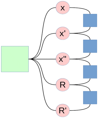
The most significant node in our algorithm is our rigid body node which embodies standard rigid body physics and is used as a center node for sensor platforms. The internal structure of this node is shown in Figure 1. In our rigid body node, we also apply limits for velocity and acceleration so that we are not calculating probabilities for impossible events. These limits are 300 m s⁻¹ for velocity and 1000 g for acceleration. The constraint equations for this node are given in Equations ((7)–(11(11) )).

Figure 1. Our rigid body node contains internal function nodes (blue) and variable nodes (red). Other nodes connect similarly to the green function node (left).

(7)

(8)

(9)

(10)

(11)

where each of x, v, a, R, and R′ are the vectors representing position, velocity, acceleration, rotation, and rotational velocity, respectively. δt_ij is the time measured from node i to node j. , , , and are the measured position, acceleration, orientation estimate, and rotational velocity as measured by the sensors, respectively. g is a vector equal to (0, 0, 9.8) m s⁻² which we use to remove the effect of gravity as measured by the accelerometer. This is in contrast to the common practice of applying a high-pass filter to remove gravity from accelerometer measurements. Instead we calculate the gravity vector using the current orientation of the sensor platform and subtract this from the acceleration reported by the accelerometer to remove the effect of gravity. This allows us to correctly report acceleration even while undergoing a constant acceleration other than gravity when the orientation is correctly reported through other means.

3.5. Graph generation

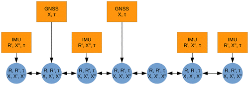
Using the nodes described above we can automatically generate and modify a graph from a data-set of sensor measurement at runtime. At this stage, we create a rigid-body node at each time-step that a data point exists. In future work we aim to cut this down to only creating a node for each time-step that we actually need access to the data.

We also create constant nodes from the sensor measurements. These constant nodes apply the calibrations and coordinate transforms described above and cache the results internally so they are not recomputed at each iteration step. A section of a generated graph is shown in Figure 2.

Figure 2. Illustration of graph generated using our technique.

Note: Rigid body nodes in blue and sensor measurement nodes in orange.

4. Results

4.1. Sensors

In this work, we have used both synthetic data and real data from a Galaxy SIII smartphone. The Galaxy SIII contains a GNSS sensor which reports at approximately 1 Hz using GPS and GLONASS. It also contains an accelerometer and gyroscope which report at approximately 100 and 200 Hz, respectively. Under the Android system, the exact reporting rate is not guaranteed however timestamps in nanoseconds are given for each of the measurements.

Our synthetic data has been generated for GNSS, Accelerometer, and Gyroscope sensors with zero offsets and reporting rates of 1, 100, and 200 Hz, respectively. This data was generated using a Gaussian distribution around the intended values with variances shown in Table 1.

Table 1. Standard deviations used for simulated data.

Parameter	x	y	z
GNSS (m)	1.000	1.000	2.000
Accelerometer (m s^−2)	0.030	0.030	0.030
Gyroscope (deg s^−1)	0.055	0.055	0.055

4.2. Calibrations used

Using the calibration described in Section 3.3 above, our calibration values for the Galaxy SIII sensors are given in Tables 2 and 3. When collecting data the GNSS sensor reported an error of 10 m, so this value was used as the variance.

Table 2. Calibration parameters for sensors.

Parameter	α	β	γ	OX	OY	OZ
Accelerometer	1.0023	0.9904	0.9888	0.1149	0.0889	0.5064
Gyroscope	1	1	1	0.0019	−0.0032	0.0017

Table 3. Measured standard deviation (SD) of sensors

Parameter	SD before calibration			SD after calibration
Axis	x	y	z	x	y	z
Accelerometer	0.0206	0.0200	0.0301	0.0206	0.0198	0.0298
Gyroscope	0.0123	0.0557	0.0054	–	–	–

4.3. Speed and accuracy

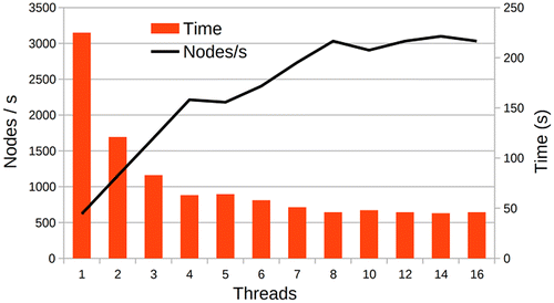
The algorithm described above has been implemented in C++ and performs at a speed of 3032 nodes per second when using 8 threads on a quad core Intel i7 920 running at 2.66 GHz. There is near linear scaling when adding more threads up to the number of virtual cores as shown in Figure 3. However, exceeding this has no value. At this stage, locks are used to synchronize the incoming message queue to each node. We are also not caching incoming messages from constant nodes, so at each iteration we need to reacquire the message from each of the constant nodes. However, with a different implementation this locking will not be required and caching can be performed which should impact performance in a positive way.

Figure 3. Performance vs. number of threads.

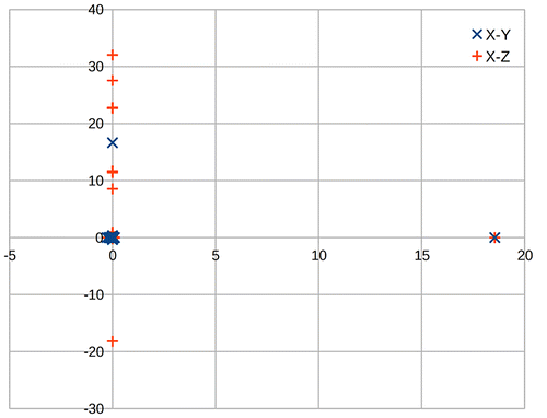
The results of our algorithm on synthetic data are presented in Figure (4). This data was generated assuming the sensor platform is stationary. Aside from a few outliers visible the vast majority of the data is centered around (0, 0, 0) despite the incoming “pseudo GNSS” data having a range of ±5 m.

Figure 4. Scatter plot of calculated positions of the sensor platform x-axis (horizontal) y/z-axis vertical.

Note: X-Y positions are shown as X marker and X-Z positions are shown as + marker.

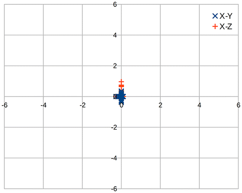
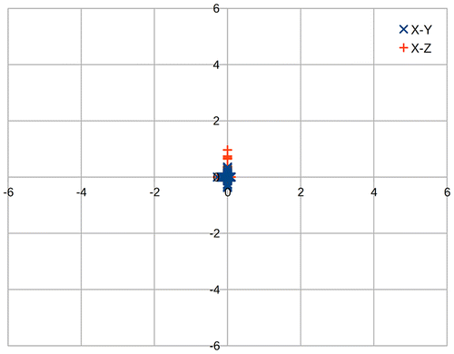
Similar to the synthetic data above, some real-world data were collected in a similar way to the synthetic data with the Galaxy SIII stationary outside with a stable GNSS lock. Figures 5 and 6 show the results of this processed data. Similar to the synthetic data above there are some outliers in the processed data. However, interestingly once these outliers are removed the resulting data is closer to the ideal (0, 0, 0).

Figure 5. Plot of calculated positions for real data.

Note: x-axis (horizontal) y/z-axis vertical. X-Y positions are shown as X marker and X-Z positions are shown as + marker.

Figure 6. Plot of calculated positions for real data.

Note: x-axis (horizontal) y/z-axis vertical. X-Y positions are shown as X marker and X-Z positions are shown as + marker.

5. Conclusions

Here, we present initial results from our proposed algorithm. While preliminary these results show that this algorithm has potential and if extended and refined may be a useful part of a sensor fusion system.

Several areas for future work have been identified. These include things such as auto calibration of sensors and time alignment of different sensors. These may be implemented as connections between sensor measurement nodes which share calibration information and time offsets, treating these values as other variables to be solved in the same way we are currently solving position and rotations.

There may also be scope to reduce the number of rigid-body nodes in our graph so we only generate one of these nodes where we need to read out the position and orientation of the platform. This may increase the speed dramatically as the number of connections would be significantly reduced hence reducing communication overhead between nodes as well as allowing for more efficient implementations of some constraint functions.

Notes on contributors

Joshua Hollick is a PhD candidate in the Department of Spatial Sciences at Curtin University. His background is in computer science and mathematics. His current research interests include photogrammetry, computer vision, and sensor fusion.

Petra Helmholz was born in Germany and educated there (Hannover, Berlin, Halberstadt), and in Australia (Melbourne). She is a lecturer in the field of Photogrammetry with the Department of Spatial Sciences at Curtin University (WASM), Perth, and a specialist in close range photogrammetry, image analysis, and photogrammetric 3D reconstruction. Her interests include automatic detection of feature classes in images, camera calibration, and applying 3D reconstruction to a number of interdisciplinary projects related to underwater environments, health and heritage mapping.

David Belton is a research fellow in the field of Photogrammetry and Laser Scanning with the Department of Spatial Sciences at Curtin University, Perth, Australia. His research focus has been in terrestrial and mobile laser scanning including areas such as feature extraction and classification of unorganized 3D point cloud data, automated techniques for point cloud processing, and geometric correction and calibration of laser scanning systems.

References

- Ali, T., P. Dutta, and H. Boruah. 2012. “A New Combination Rule for Conflict Problem of Dempster-Shafer Evidence Theory.” International Journal of Energy, Information and Communications 3 (1): 35–40.
- Ayub, S., A. Bahraminisaab, and B. Honary. 2012. “A Sensor Fusion Method for Smart Phone Orientation Estimation.” In Proceedings of the 13th Annual Post Graduate Symposium on the Convergence of Telecommunications, Networking and Broadcasting, Liverpool, June 25−26.
- Crandall, D. J., A. Owens, N. Snavely, and D. P. Huttenlocher. 2013. “SfM with MRFs: Discrete-continuous Optimization for Large-scale Structure from Motion.” IEEE Transactions on Pattern Analysis and Machine Intelligence 35 (12): 2841–2853.10.1109/TPAMI.2012.218
- Ihler, A. T., J. Iii, and A. S. Willsky. 2005. “Loopy Belief Propagation: Convergence and Effects of Message Errors.” Journal of Machine Learning Research 6: 905–936.
- Jøsang, A., and S. Pope. 2012. “Dempster’s Rule as Seen by Little Colored Balls.” Computational Intelligence 28 (4): 453–474.10.1111/coin.2012.28.issue-4
- Kerl, C., J. Sturm, and D. Cremers. 2013. “Robust Odometry Estimation for RGB-D Cameras.” In International Conference on Robotics and Automation (ICRA), 3748−3754, Karlsruhe, Germany, May 6–10, IEEE.
- Klein, L. A. 1999. Sensor and Data Fusion Concepts and Applications. Bellingham, WA: SPIE Optical Engineering Press.
- Koks, D., and S. Challa. 2003. An Introduction to Bayesian and Dempster-Shafer Data Fusion. Technical report DSTO-TR-1436. http://dspace.dsto.defence.gov.au/dspace/bitstream/1947/4316/5/DSTO-TR-1436%20PR.pdf.
- Lhuillier, M. 2012. “Incremental Fusion of Structure-from-Motion and GPS Using Constrained Bundle Adjustments.” IEEE Transactions on Pattern Analysis and Machine Intelligence 34 (12): 2489–2495.10.1109/TPAMI.2012.157
- Murphy, K. P., Y. Weiss, and M. I. Jordan. 1999. “Loopy Belief Propagation for Approximate Inference: An Empirical Study.” In Proceedings of the Fifteenth Conference on Uncertainty in Artificial Intelligence, 467−475, Stockholm, July 30−August 1.
- Pearl, J. 1982. “Reverend Bayes on Inference Engines: A Distributed Hierarchical Approach.” In Proceedings of American Association for Artificial Intelligence, 133–136, Pittsburgh, Pennsylvania, August 18–20.
- Sudderth, E. B., A. T. Ihler, W. T. Freeman, and A. S. Willsky. 2003. “Nonparametric Belief Propagation.” In Conference on Computer Vision and Pattern Recognition, 605−612, Madison, Wisconsin, June 18–20, IEEE.
- Tundo, M. D., E. Lemaire, and N. Baddour. 2013. “Correcting Smartphone Orientation for Accelerometer-Based Analysis.” In 2013 IEEE International Symposium on Medical Measurements and Applications Proceedings (MeMeA), 58−62, Gatineau, QC, Canada, May 4−5.
- Yedidia, J. S., W. T. Freeman, and Y. Weiss. 2000. “Generalized Belief Propagation.” In Neural Information Processing Systems, 689−695. Denver, Colorado, MIT Press, November 28–30.
- Yedidia, J. S., W. T. Freeman, and Y. Weiss. 2003. “Understanding Belief Propagation and Its Generalizations.” In Exploring Artificial Intelligence in the New Millennium, Volume 8, edited by G. Lakemeyer and B. Nebel, 236−239. Burlington: Morgan Kaufman Publishers.