The applications of robust estimation method BaySAC in indoor point cloud processing

Abstract

Based on Bayesian theory and RANSAC, this paper applies Bayesian Sampling Consensus (BaySAC) method using convergence evaluation of hypothesis models in indoor point cloud processing. We implement a conditional sampling method, BaySAC, to always select the minimum number of required data with the highest inlier probabilities. Because the primitive parameters calculated by the different inlier sets should be convergent, this paper presents a statistical testing algorithm for a candidate model parameter histogram to compute the prior probability of each data point. Moreover, the probability update is implemented using the simplified Bayes’ formula. The performances of the BaySAC algorithm with the proposed strategies of the prior probability determination and the RANSAC framework are compared using real data-sets. The experimental results indicate that the more outliers contain the data points, the higher computational efficiency of our proposed algorithm gains compared with RANSAC. The results also indicate that the proposed statistical testing strategy can determine sound prior inlier probability free of the change of hypothesis models.

Keywords:

• 3D indoor modeling
• robust estimation
• RANSAC
• BaySAC
• point cloud registration
• fitting of point cloud

1. Introduction

A 3D model of an indoor environment includes modeling of indoor space, floor, wall and objects inside a room. These 3D models will play a more important role in context aware and robotics applications such as automatic route tracking, object detection, etc. Range camera (e.g. Kinect) has been proven to be an applicable sensor for 3D indoor modeling (Henry et al. 2012; Khoshelham and Elberink 2012; Camplani, Mantecon, and Salgado 2013). The estimation of the parameters of a model is often involved in the data processing for 3D model reconstruction (e.g. the geometric model of an indoor feature in the fitting of point clouds, the rigid transformation model in point cloud registration, and so on). Because the point clouds and images acquired from an indoor scene always contain plenty of noises, it is necessary to implement the robust estimation of the parameters of a model. RANdom SAmple Consensus (RANSAC) (Fischler and Bolles 1981) is a well-regarded technique for the segmentation and fitting of laser scanning data, because it is proven to be capable of addressing more than 50% of all outliers.

R-RANSAC (Matas and Chum 2004) was proposed to increase the model parameter estimation speed through hypothesis evaluation randomization processes because numerously erroneous model parameters are expected to arise from contaminated samples evaluated in RANSAC. Schnabel, Wahl, and Klein (2007) improved the efficiency of RANSAC through local point selection and the incorporation of a simplified score function. Torr and Zisserman (2000) applied the robust estimation method of Maximum Likelihood Estimation SAmple Consensus (MLESAC) to identify best-fitting roof models in a model-driven manner. Torr and Davidson (2003) presented IMPortance sampling and random SAmple Consensus (IMPSAC) method, which employed a hierarchical resampling algorithm. Li et al. (2014) improved the RANSAC strategy by defining a prior energy function to optimize sampling strategy. A normal-coherence CC-RANSAC (NCC-RANSAC) was presented to perform a normal coherence check before RANSAC process to remove the data points with contradictory normal directions to the fitted plane (Qian and Ye 2014). İmre and Hilton (2015) proposed order statistics of RANSAC, which obviated the noise-free data assumption. Xu et al. (2016) proposed a weighted RANSAC approach, which designed weight functions in terms of the difference in the error distribution between the proper and improper plane hypotheses.

A conditional sampling method, Bayesian Sampling Consensus (BaySAC) (Botterill, Mills and Green 2009) was presented to always select the minimum number of required data with the highest inlier probabilities as a hypothesis set for the purpose of reducing the number of iterations needed to find a good model. However, Botterill, Mills, and Green (2009) admitted that there was a possibility that degenerate configurations incorrectly assumed to contain outliers could cause a sampling strategy to fail.

To improve the robustness and applicability of the original BaySAC method, Kang et al. (2014) optimized the BaySAC algorithm by presenting a model-free algorithm of statistical testing of candidate model parameters to compute the prior probability of each data point. Therefore, in this paper we apply the above method in the processing of indoor point clouds, i.e. point cloud registration and fitting.

2. Optimized BaySAC

In the BaySAC algorithm, a hypothesis set is only tried if at that moment it is the most likely one to be correct, which is determined in terms of its inlier probability. BaySAC assumes independence between the different inlier probabilities of data points in the same hypothesis set. First, the minimum number of data required with the highest inlier probabilities is selected as the hypothesis set. After evaluating a hypothesis set, the inlier probabilities of the data points of the hypothesis set are updated using Bayes’ rule. The hypothesis set evaluation is consecutively repeated with the new inlier probabilities. Although the determination and evaluation of the probabilities also takes some time, this strategy can remarkably reduce the number of iterations needed to find a good model, and is hence reducing the computational costs. Compared with RANSAC, the key properties of BaySAC are to determine and update the inlier probabilities of the data points.

2.1. Determination of the prior inlier probabilities of data points

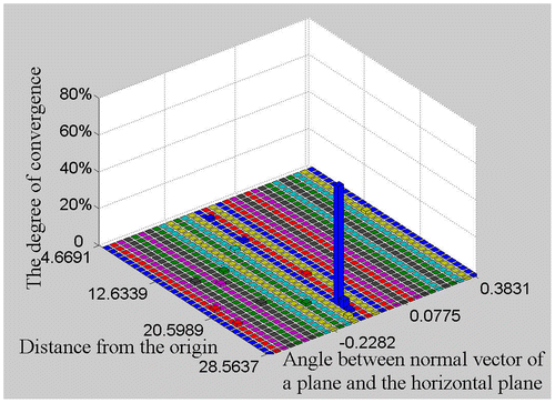
The statistical testing process proposed by Kang et al. (2014) is generic and can be applied to any BaySAC problem. The process is based on a histogram to dynamically evaluate the convergence of the hypothesis parameters sets during the hypothesis testing process. Figure 1 shows a histogram to evaluate the convergence of the planar parameters for point cloud fitting. The horizontal and vertical axes of Figure 1 denote the angle between the normal vector n of a plane and the horizontal plane, and the perpendicular distance from the origin ρ, respectively. The upright axis represents the convergence degree of each set of parameters. Different convergent cluster of the hypothesis sets will be presented in the histogram. We select the oldest parameter set as the reference point for each convergent cluster of parameter sets. The more the hypothesis sets converge to a cluster, the more possible is it that the reference parameters set of the cluster is correct. Therefore, the convergence degree of a cluster is presented to evaluate the correct possibility. The convergence degree is a percentage which describes that the number of sets converges to a parameter set cluster. It is calculated by dividing the number of the hypothesis sets in the cluster by the total number of hypothesis sets.

Figure 1. 2D hypothesis model parameters histogram of a plane.

In this paper, the geometric model of an indoor feature in the fitting of point clouds and the rigid transformation model in point cloud registration are used as the hypothesis models.

When the degree of convergence of a cluster in the distribution of parameter solutions reaches a predefined threshold, the first hypothesis set in that cluster is used to determine the prior inlier probabilities of the data points according to Equation (1(1) ):(1)

where P_i denotes the prior probability of point i, D_i is the distance between point i and the fitted primitive, and m represents the predefined threshold for outlier identification, which is set as five times the point precision.

2.2. Probability updating

After determining the prior inlier probabilities of each data point, the following Equation (2(1) ) is employed to update the inlier probabilities during consecutive iterations (Kang et al. 2014):(2)

where I is the set of all inliers, H_t is the hypothesis set of n data points used in iteration t of the hypothesis testing process, P_t−1 (i∈I) and P_t (i∈I) denote the inlier probabilities for data point i during iterations t₋1 and t, respectively, k is the number of points consistent with the model during a test, and D is the total number of data points.

2.3. The implementation of optimized BaySAC

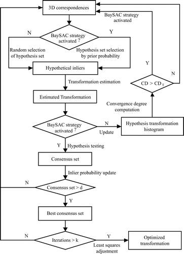
Figure 2 shows the flow chart of optimized BaySAC (taking point cloud registration as an example). The process first starts with a RANSAC strategy, which chooses an initial data-set randomly from the candidate points. Meanwhile, the proposed convergence evaluation is iteratively implemented using the newly calculated hypothesis parameter set. During each iteration, we update the degrees of convergence of all candidate parameter sets in terms of the newly calculated hypothesis parameter set. If the highest degree of convergence exceeds the predefined threshold (CD_T in Figure 2), its corresponding parameter set is used to determine the prior inlier probabilities of data points using Equation (2(1) ). The BaySAC strategy is then activated. If the number of iterations RANSAC needs is very small, it is likely that the highest degree of convergence fails to exceed the threshold when the RANSAC process ends. In this case, the BaySAC degrades to RANSAC. Once the BaySAC strategy is activated, the hypothesis testing process is implemented as the procedure explained in Section 2.2.

Figure 2. Flowchart of BaySAC-CONV algorithm.

3. Experimental results

To demonstrate the application of the method proposed by Kang et al. (2014), we conducted experiments with three sets of indoor point clouds, acquired respectively by the 3D SwissRanger camera, by Kinect 2.0 and by the LMS-Z620 laser scanner from RIEGL. The SwissRanger data-set consists of two point clouds sampling the indoor environment of a building (Data-set I). Kinect 2.0 data-set comprises a registered point cloud from 61 scans captured in a room with an average shift of 0.4 m between the scanning centers (Data-set II). LMS-Z620 data-set was captured from an underground parking garage (Data-set III).

3.1. Point cloud registration

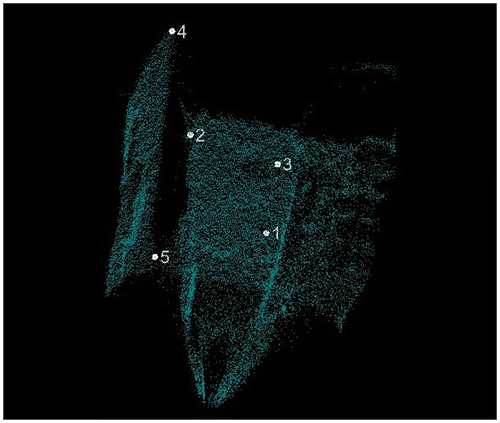
The performance of the BaySAC-CONV algorithm in point cloud registration was evaluated on Data-set I in terms of both registration accuracy and computational efficiency. Correspondences between different scans were identified using reflectance images (as shown in Figure 3). The registration accuracies of RANSAC and BaySAC-CONV were evaluated using the average distance between inlier correspondences after registration. Figure 4 shows that five correspondences are identified as check points. Table 1 lists the evaluation of registration accuracies in terms of the average distance between the selected correspondences after registration. BaySAC-CONV achieved higher accuracy (23.3 mm) compared with the performance of the plain RANSAC (50.2 mm).

Figure 3. Identified 3D correspondences: (a) Correspondences in scan A; (b) Correspondences in scan B.

Figure 4. Illustration of check points.

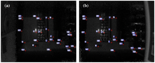
Table 1. Evaluation of registration accuracy in terms of average point-to-point distance.

Point cloud	Number of Check Points	RMS (RANSAC)	RMS (BaySAC-CONV)
Data-set I	5	50.2 mm	23.3 mm

Hypothesis set evaluation is an iterative process, and therefore the calculational efficiency of the proposed strategies is evaluated in terms of the number of iterations and computation time. As described in Section 2.3, the BaySAC-CONV strategy consists of two parts, i.e. the random part (BaySAC-CONV-Random) and the BaySAC part. The random part consists of the iterations implemented with a RANSAC strategy, during which the inlier probabilities of the different correspondences are determined.

As shown in Table 2, the ratio between the number of inliers and that of possible correspondences in Data-set I reaches 81%. The number of iterations for RANSAC varies from 6 to 18. The total number of iterations for BaySAC-CONV varies from 2 to 11.

Table 2. Computational efficiencies of the proposed strategies (Iteration).

Point cloud	Possible Correspondences	I/C ratio	Iterations (RANSAC)	Iterations (BaySAC-CONV)
				Random	Total
Data-set I	48	81%	6–18	1–6	2–11

The average consumed time of the two strategies is listed in Table 3. The random parts of the time consumed by BaySAC-CONV is to determine the prior inlier probabilities of data points, which are the core of BaySAC-CONV. After the determination of the prior inlier probabilities, the use of BaySAC remarkably reduces the computational time needed to find a good model compared with the time consumed by plain RANSAC. For instance, in Table 3, 5 ms are spent by BaySAC-CONV to find a good transformation from Data-set I, while the time cost by plain RANSAC is 21 ms.

Table 3. Computational efficiencies of the proposed strategies (unit: ms).

Point cloud	Time of RANSAC	Time of BaySAC-CONV
		Random	Total
Data-set I	21	3	5

3.2. Fitting of point clouds

We used the RANSAC and BaySAC-CONV methods for planar primitive fitting of Data-sets II and III. The fitting results are shown in Figures 5 and 6, respectively.

Figure 5. Comparison of the fitting results of different methods on Data-set II: (a) RANSAC; (b) BaySAC-CONV.

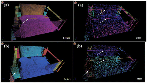
Figure 6. Comparison of the fitting results of different methods before and after the point cloud simplification of Data-set III: (a) RANSAC; (b) BaySAC-CONV.

To validate the accuracy of the plane fitting, we selected correct points that were not involved in the fitting as check points. We solved for the distances from the check points to the fitting plane and computed the median error. We also evaluated the performance of different algorithms based on accuracy and computational cost. Table 4 lists the median errors and fitting times of the planar primitive fitting on Data-sets II and III. The fitting accuracy of the BaySAC-CONV algorithm is not considerably different from that of the RANSAC algorithms, while the efficiencies of the BaySAC-CONV algorithms are higher than that of the RANSAC algorithm.

Table 4. Comparison of fitting results.

Point cloud	Method	Number of fitting planes	Average median error (m)	Fitting time (ms)
Data-set II	RANSAC	2707	0.028	3889
	BaySAC-CONV	1943	0.028	2540
Data-set III	RANSAC	48	0.0049	1492
	BaySAC-CONV	48	0.0074	337

Data-set III contains many planar features, and therefore we analyze the point cloud in one region (Figure 6). Figure 6 includes images of the analyzed region. Compared with the results of the original point cloud, finer planar primitives were detected owing to the simplification preserving the feature points, which enhanced the prominence of small-sized feature after simplification (highlighted with the white arrows in the “before” parts of Figures 6(a) and (b)).

4. Conclusions

In this paper, an optimized BaySAC algorithm is applied in the processing of indoor point clouds, which developed a strategy for determining the prior probability from the statistical characteristics of the deterministic mathematical model for hypothesis testing. The performances of the BaySAC algorithm with the proposed strategies of the prior probability determination and the RANSAC framework are compared using real data-sets in terms of computational efficiency and accuracy. The experimental results indicate that the optimized BaySAC algorithm can achieve better performances than RANSAC in both accuracy and computational efficiency. The more outliers contain the data points, the higher computational efficiency of the optimized BaySAC algorithm gains compared with RANSAC. The results also indicate that the statistical testing strategy can determine sound prior inlier probability free of the changes of hypothesis models. In the future, this method will be expanded to the fitting of complex features, which will also increase the adaptability of the proposed method.

Funding

This research was supported by the National Natural Science Foundation of China [grant number 41471360] and the Fundamental Research Funds for the Central Universities [grant number 2652015176].

Notes on contributor

Zhizhong Kang, PhD in photogrammetry and remote sensing from Wuhan University, China, in 2004 worked as a postdoctoral researcher with Delft University of Technology, Delft, the Netherlands from 2006 to 2008. Currently, he is an associate professor and the head with the Department of Remote Sensing and Geo-Information Engineering, China University of Geosciences, Beijing, China. He has authored more than 60 referred journal and conference publications. His research interests include digital photogrammetry and computer vision including vehicle-based image sequence processing, laser scanning data processing, and lunar structure recognition and extraction. Kang has served as Regional Coordinator for Asia of ISPRS WG V/3 and Member of Committee on Photogrammetry and Remote Sensing, Chinese Society for Geodesy Photogrammetry and Cartography. He was the recipient of 2015 ERDAS Award for Best Scientific Paper in Remote Sensing by ASPRS, for the paper “Z. Kang, F. Jia, L. Zhang, A robust image matching method based on optimized BaySAC, Photogrammetric Engineering & Remote Sensing, vol. 80, No. 11, pp. 1041–1052, 2014.”

References

- Botterill, T., S. Mills, and R. Green. 2009. “New Conditional Sampling Strategies for Speeded-up RANSAC.” In Proceeding of the British Machine Vision Conference (BMVC 2009), London, UK, September 7–10.
- Camplani, M., T. Mantecon, and L. Salgado. 2013. “Depth-color Fusion Strategy for 3-D Scene Modeling with Kinect.” IEEE Transactions on Cybernetics 43 (6): 1560–1571.10.1109/TCYB.2013.2271112
- Fischler, M. A., and R. C. Bolles. 1981. “Random Sample Consensus: A Paradigm for Model Fitting with Applications to Image Analysis and Automated Cartography.” Communications of the ACM 24 (6): 381–395.10.1145/358669.358692
- Henry, P., M. Krainin, E. Herbst, X. F. Ren, and D. Fox. 2012. “RGB-D Mapping: Using Kinect-style Depth Cameras for Dense 3D Modeling of Indoor Environments.” The International Journal of Robotics Research 31 (5): 647–663.10.1177/0278364911434148
- İmre, E., and A. Hilton. 2015. “Order Statistics of RANSAC and Their Practical Application.” International Journal of Computer Vision 111 (3): 276–297.10.1007/s11263-014-0745-1
- Kang, Z. Z., L. Zhang, B. Wang, Z. Li, and F. Jia. 2014. “An Optimized BaySAC Algorithm for Efficient Fitting of Primitives in Point Clouds.” IEEE Geoscience and Remote Sensing Letters 11 (6): 1096–1100.10.1109/LGRS.2013.2286856
- Khoshelham, K., and S. O. Elberink. 2012. “Accuracy and Resolution of Kinect Depth Data for Indoor Mapping Applications.” Sensors 12 (2): 1437–1454.10.3390/s120201437
- Li, B., D. L. Ming, W. W. Yan, X. Sun, T. Tian, and J. W. Tian. 2014. “Image Matching Based on Two-column Histogram Hashing and Improved RANSAC.” IEEE Geoscience and Remote Sensing Letters 11 (8): 1433–1437.
- Matas, J., and O. Chum. 2004. “Randomized RANSAC with Td, D Test.” Image and Vision Computing 22 (10): 837–842.10.1016/j.imavis.2004.02.009
- Qian, X. F., and C. Ye. 2014. “NCC-RANSAC: A Fast Plane Extraction Method for 3-D Range Data Segmentation.” IEEE Transactions on Cybernetics 44 (12): 2771–2783.10.1109/TCYB.2014.2316282
- Schnabel, R., R. Wahl, and R. Klein. 2007. “Efficient RANSAC for Point-Cloud Shape Detection.” Computer Graphics Forum 26 (2): 214–226.10.1111/cgf.2007.26.issue-2
- Torr, P. H. S., and A. Zisserman. 2000. “MLESAC: A New Robust Estimator with Application to Estimating Image Geometry.” Computer Vision and Image Understanding 78 (1): 138–156.10.1006/cviu.1999.0832
- Torr, P. H. S., and C. Davidson. 2003. “IMPSAC: Synthesis of Importance Sampling and Random Sample Consensus.” IEEE Transactions on Pattern Analysis Machine Intelligence 25 (3): 354–364.10.1109/TPAMI.2003.1182098
- Xu, B., W. S. Jiang, J. Shan, J. Zhang, and L. L. Li. 2016. “Investigation on the Weighted RANSAC Approaches for Building Roof Plane Segmentation from LiDAR Point Clouds.” Remote Sensing 8 (5). doi:10.3390/rs8010005.