Improving global land cover characterization through data fusion

Abstract

Global-scale land cover characterization has advanced from a spatial resolution of 1 × 1° in the mid-1990s to 30 × 30 m resolution to date. However, some mapping challenges exist persistently regardless of the increasing spatial resolution. Data fusion has been proved as an effective way of improving land cover characterization. Here we applied a machine learning-based data integration approach for improving global-scale forest cover characterization. The approach employed six coarse-resolution (250–1000 m) global land cover maps as input and various regional, higher-resolution land cover data-sets as reference to build regression tree models per continent. The average error of 10-fold cross validation of the regression tree models varied between 7.70 and 15.68% forest cover and the r² varied between 0.76 and 0.94, indicating the robustness of the trained models. As a result of data fusion, the synthesized global forest cover map was more accurate than any input global product. We also showed that other major vegetative land cover types such as cropland, woodland, grassland, and wetland all exhibit similar magnitude of discrepancies as forest among existing land cover maps. Our developed method, because of its type- and scale-invariant feature, can be implemented for other land cover types for improving their global characterization. The ensemble approach can also be internalized for improving data quality when generating a global land cover product, where multiple versions can be produced and subsequently integrated.

Keywords:

• Satellite
• remote sensing
• land cover
• data fusion
• regression tree
• global

1. Introduction

Changes in land cover and land use significantly affect earth system functions and processes including the carbon cycle, the hydrological cycle, biodiversity, and socioeconomic development (Bonan 2008; Foley et al. 2005; Pan et al. 2011; Pimm et al. 2014; Song et al. 2015). Optical satellite imagery is the primary data source for characterizing land cover and monitoring land cover change at the global scale (Townshend et al. 2012). Research on characterizing global patterns of land cover using remotely sensed data has been conducted since the mid-1990s. Early efforts were focused on generating coarse-resolution (250 m−1 km) land cover maps for the main purpose of providing land surface boundary conditions to biogeochemical modeling. These products include Global Land Cover Characterization (GLCC) (Loveland et al. 2000), the University of Maryland land cover (UMD LC) (Hansen et al. 2000), Global Land Cover 2000 (GLC2000) (Bartholomé and Belward 2005), the Moderate Resolution Imaging Spectroradiometer land cover (MODIS LC) (Friedl et al. 2002), the MODIS Vegetation Continuous Fields (MODIS VCF) (Hansen et al. 2003), and the GlobCover land cover product (Bicheron et al. 2008). Taking the forest class as an example, substantial disagreement in their representation of global forest was observed due to their inconsistent definitions of forest, their coarse spatial resolutions and the diversity of satellite data and methods used in deriving these map products (Figure 1(a)).

Figure 1. Highlighting the agreement and disagreement of existing coarse resolution (250 m−1 km) and fine resolution (30 m) land cover products for forest/tree cover characterization.

Notes: (a) Agreement map of six coarse-resolution land cover products on forest cover. The six maps are GLCC, UMD LC, GLC2000, MODIS LC, MODIS VCF, and GlobCover. Values in the legend represent the total amount of products that classify a given pixel as forest, regardless of leaf type or leaf longevity. (b) Difference of two Landsat-based global tree cover maps. The two maps are the Global Land Cover Facility (GLCF) tree cover produced by Sexton et al. (2013) and the Global Land Analysis and Discovery (GLAD) tree cover developed by Hansen et al. (2013), both of which estimate percent tree cover at 30-m spatial resolution. Per-pixel absolute difference of the two tree cover values were calculated and divided by the GLCF tree cover to derive the normalized difference, which was overlaying on GLCF tree cover to create the map. Only data over forested regions with GLCF tree cover ≥10% and normalized difference ≥50% were shown to highlight the maximum difference of the two products. A clear resemblance was noticed between (a) and (b).

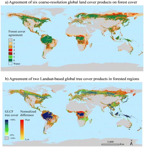
Global-scale land cover mapping at 30 m resolution has only become feasible in recent years, owing much to the United States Geological Survey (USGS)’s open Landsat data policy (Wulder et al. 2012) and the reduced cost of data storage and computation. So far, five 30 m resolution global land/forest/tree cover maps have been generated by Chen et al. (2014), Gong et al. (2013), Hansen et al. (2013), Kim et al. (2014), and Sexton et al. (2013) and more data-sets are in production (Giri et al. 2013; Townshend et al. 2012). The spatial details revealed by these Landsat-based map products are 100–1000 times finer than those coarse-resolution maps and the cross-map consistency has improved considerably because of the common data source. Characterizing continuous tree cover (Hansen et al. 2013; Sexton et al. 2013) instead of forest cover also eliminates the definitional ambiguity of forest (Sexton et al. 2016). However, the overall global disagreement pattern of the two Landsat-based tree cover data-sets resembles to a noticeable degree those coarse-resolution forest cover data-sets (Figure 1(b)), highlighting the persistent challenge of global-scale land cover characterization in specific regions, such as the dry tropical woodlands in South America and Africa and the transition ecotones in boreal North America and Eurasia.

Increasing the spatial resolution of mapping represents a continued advancement in land cover research. With the open access to standardized, pre-processed Landsat and Sentinel data and the emerging cloud-based computing platforms (e.g. Google Earth Engine, Amazon Web Services), the amount of global-scale land cover maps at medium spatial resolution (10−30 m) can only be expected to proliferate in the coming years. These forthcoming data-sets would likely have discrepancies as has been witnessed with the coarse-resolution data, perhaps concentrated in similar geographic regions. Therefore, exploratory questions can always be asked, for example, what are the implications of the observed agreement and disagreement patterns among different data-sets for future land cover mapping? Can these diverse data-sets, each of which has its unique advantage and as a collection has a reasonable level of agreement, be synthesized to generate a more accurate land cover map, regardless of their spatial resolutions?

Several studies have attempted to adopt a data harmonization approach for improving land cover mapping. Jung et al. (2006) integrated multiple versions of GLC2000, GLCC, and MODIS land cover maps by cross-walking different land cover legends and created a joint 1-km land cover map for carbon cycle modeling research. Fritz et al. (2011) developed a synergy approach and created a hybrid cropland map for Africa. The method was recently expanded to the global scale (Fritz et al. 2015; Waldner et al. 2016). Schepaschenko et al. (2011) created a hybrid land cover data-set over Russia by combing satellite-based land cover maps, national statistics as well as in situ information. Recently, Schepaschenko et al. (2015) employed geographically weighted regression and generated a 1-km resolution global hybrid forest mask by integrating remote sensing, crowdsourcing, and national statistics from the United Nations Food and Agricultural Organization (FAO). Latham et al. (2014) produced the FAO Global Land Cover-SHARE database, a 1-km land cover map, by harmonizing various global and regional land cover data-sets following rules defined in FAO’s Land Cover Classification System (LCCS) (Di Gregorio and Jansen 2005). Tsendbazar, de Bruin, and Herold (2016) applied a regression kriging method to integrate four global land cover products and publicly available reference data for deriving user-specific maps. Song et al. (2014) developed a machine learning-based data fusion approach and created an improved continuous forest cover map over North America. By extending our previous efforts (Song et al. 2014), here in this paper we applied the well-tested method to other continents and provided a demonstration of global-scale applications.

2. Data and methods

Our overall data integration methodology follows Song et al. (2014). As an extension to the previous work, here we first provide a detailed review of the various global and regional land cover products used in this research. Key steps of the data integrated approach are then briefly summarized.

2.1. Global land cover products

2.1.1. Global land cover characterization

The GLCC database was developed at a continent-by-continent basis (Loveland et al. 2000). Advanced Very High Resolution Radiometer (AVHRR) 10-day Normalized Difference Vegetation Index (NDVI) composites for the period of April 1992 to March 1993 were aggregated into monthly maximum NDVI composites to minimize cloud contamination. Non-vegetated land covers such as barren land, snow, and ice were identified using thresholds of the maximum NDVI and were masked prior to classification. Water bodies and urban land cover were not classified from AVHRR, but imported from the hydrography layer and populated places data layer from the Defense Mapping Agency’s Digital Chart of the World (DCW) (Danko 1992). An unsupervised algorithm was applied to cluster the masked AVHRR monthly composites and each cluster was labeled as one of the 961 seasonal land cover regions. Each seasonal land cover region was firstly translated into Olson’s Global Ecosystems Legend (Olson 1994) and then cross-walked into six different land cover legends, including the International Geosphere-Biosphere Programme (IGBP) scheme and the USGS Anderson scheme.

2.1.2. University of Maryland land cover

The UMD LC was also generated from AVHRR data but with a supervised classification procedure (Hansen et al. 2000). The 1-km AVHRR 10-day NDVI composites and the five optical bands were used to create a total of 41 annual metrics including the maximum, minimum, and mean NDVI as well as pixel values of channels 1–5 associated with the eight greenest and the four warmest months. Training data were derived from a total of 156 60 m Landsat Multispectral Scanner images. A decision tree model was trained and applied to the annual metrics to create vegetation classifications. The urban and built-up class was taken from GLCC, which was in turn taken from DCW. The UMD product employed a classification scheme modified from IGBP for use with the Simple Biosphere (SiB) general circulation model (Sellers et al. 1986). Since the SiB scheme did not include agricultural mosaics, wetlands, snow, and ice classes, these classes were not explicitly characterized. Instead, the snow and ice class was contained in the bare ground class.

2.1.3. Global land cover 2000

The GLC2000 project was initialized by the European Union’s Joint Research Center with the objective of producing a land cover map for the International Conventions on Climate Change, the Convention to Combat Desertification, the Ramsar Convention, and the Kyoto Protocol (Bartholomé and Belward 2005). Input data were based on SPOT-4 VEGETATION VEGA2000 acquired from November 1999 to December 2000. The whole globe was divided into 19 regions. Classification for each region was carried out by local experts using independent methods and legends that were most appropriate for the respective region. Subsequently, regional land cover classes were translated to a global legend according to FAO’s LCCS (Di Gregorio Jansen 2005). Some parts of global classification were further improved using ancillary data such as digital elevation and nighttime lights data.

2.1.4. MODIS land cover

One of the standard MODIS products is the global land cover map (MCD12Q1) generated at Boston University. Multiple versions of this product have been generated, all of which employed a supervised decision tree algorithm (Friedl et al. 2002, 2010). Input data and features included the nadir Bidirectional Reflectance Distribution Function (BRDF)-adjusted reflectance data, land surface temperature, enhanced vegetation index, and annual metrics (minimum, maximum, and mean) of each band. Training data were derived from Landsat images taken from the System for Terrestrial Ecosystem Parameterization database, which included 1860 sites distributed across the globe. The final map was a result of an iterative boosting procedure – an ensemble classification method in which multiple classifications were carried out based on resampled training data and the final classification was determined by an accuracy-weighted vote. The product is available in multiple land cover legends, including the IGBP scheme, the UMD scheme, the MODIS leaf area index/fraction of photosynthetically active radiation class system (Myneni et al. 2002), an 8-biome classification system (Running et al. 1995), and a 12-class plant functional type system (Bonan et al. 2002). The map in IGBP legend was used in this study.

2.1.5. MODIS vegetation continuous fields

The MODIS vegetation continuous fields (VCF) product is also a standard MODIS land product (MOD44B). It estimates fractional vegetation cover at sub-pixel level, representing a theoretically advanced characterization of land cover over categorical maps. The latest version was generated at a spatial resolution of 250 m annually from 2000 to 2010 (DiMiceli et al. 2011). Following an established method described in Hansen et al. (2003), bagged regression tree models were trained using a large Landsat-based reference sample and annual phenological metrics composited from the 16-day surface reflectance. The models were applied to annual metrics to predict percent tree, herbaceous or bareground cover per MODIS pixel per year. Poor pixels which were either cloud, cloud shadow, high aerosol or had a view zenith angle >45° were reduced through the composition process and the remnant were flagged in the quality assurance layer. White, Shaw, and Ramsey (2005) validated the Collection 1 MODIS VCF using independent field data across the arid southwestern United States. Montesano et al. (2009) evaluated the Collection 4 product using reference data derived from high-resolution images across the boreal-taiga ecotone. Sexton et al. (2013) estimated the error of Collection 5 VCF against measurements of tree cover from small-footprint Lidar data in four sites across three different forest biomes and found that the root-mean-square-error of Collection 5 VCF ranged from 7 to 21% tree cover. Recently, Song et al. (2014) showed that the annual MODIS VCF product had high temporal precision, which allowed to map global forest cover change at an annual resolution.

2.1.6. GlobCover land cover

The GlobCover project, conducted by the European Space Agency, was designed to generate a land cover map of the world using 300 m data from the Medium Resolution Imaging Spectrometer Instrument on-board the ENVISAT satellite (Bicheron et al. 2008). Input data were acquired for the period between December 2004 and June 2006. Cloud-free surface reflectance mosaics were generated through a series of pre-processing steps including geometric correction, cloud and shadow screening, land/water classification, atmospheric correction, BRDF correction, and temporal compositing. The mosaics were stratified into bioclimatically homogenous regions across the world and subsequently converted to land cover maps region by region. The overall classification procedure consisted of a supervised step and an unsupervised step. Land cover classes that were not well represented such as urban and wetland, were classified with a supervised algorithm and the remaining pixels were clustered with an unsupervised algorithm. Clusters with similar temporal features were grouped into a manageable number of spectral-temporal classes and then labeled to land cover types following the LCCS. Some local land cover products were used as reference to fine-tune the global map as a post-classification step. Flooded forests, which were largely underestimated, were directly imported from the regional data. Delineation of water bodies was improved by incorporating the Shuttle Radar Topography Mission Water Body Data.

2.2. Regional high-resolution land cover data-sets

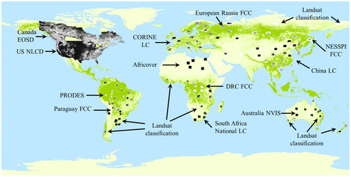
The overall data fusion strategy was to leverage as much as possible existing, regional, high-resolution land cover products. Those regional data-sets were most likely of higher quality than global data-sets over the corresponding regions because they were usually produced by local experts or experts who specialized in the study area. Therefore, regional products could be used as training data in supervised machine learning models, as has been shown in North America (Song et al. 2014). However, existing data-sets often do not have a representative spatial distribution over a continent. Thus, we classified a total of 28 Landsat images as forest/non-forest maps to augment the training data-set, especially in underrepresented ecoregions. The developed methodology was applied to the global scale at a continent-by-continent basis except Antarctica.

We collected various regional land cover maps at sub-100 meter resolution around the globe (Figure 2). The National Land Cover Database (NLCD) over the Conterminous United States (Homer et al. 2004) and the Earth Observation for Sustainable Development of Forests (EOSD) forest cover map over Canada (Wulder et al. 2008) were used in North America. The PRODES deforestation maps over the Brazilian Amazon (http://www.obt.inpe.br/prodes/index.php) and the Paraguay forest cover change (FCC) data-set (Huang et al. 2009) were used in South America. To achieve a representative geographical distribution of the reference data, we also added Landsat-based forest/non-forest maps, which were derived through a clustering-labeling approach. These augmented training sites were located in a variety of ecosystems including the Brazilian Cerrado, tropical montane forests in Colombia, agricultural areas in Uruguay, temperate forests in southern Chile, and desert in northern Chile. Similarly, the vector-based Africover database (http://www.glcn.org/activities/africover_en.jsp), the 60 m resolution FCC product over Democratic Republic of the Congo (DRC) (Potapov et al. 2012), the South African National Land Cover product (Fairbanks et al. 2000), and augmented training sites were used in Africa. The CORINE Land Cover database over Europe (Bossard, Feranec, and Otahel 2000), the 60 m FCC product over European Russia (Potapov, Turubanova, and Hansen 2011), China’s National Land Cover (Liu et al. 2002), and the FCC data-sets generated by the Northern Eurasia Earth Science Partnership Initiative were employed in Eurasia (Pflugmacher et al. 2011). The Australian National Vegetation Information System Major Vegetation Groups map (Thackway et al. 2007) and augmented Landsat-based training data were used in Oceania.

Figure 2. Regional land cover data-sets collected or generated for the integration of global land cover products. Black-and-white layer shows the location of each regional data-set, whereas the green background layer is the MODIS VCF tree cover.

Notes: For North America, two national-scale wall-to-wall products EOSD and NLCD were shown on the map but only a subsample of the data-sets was used as training in the integration model Song et al. (2014), the amount of which was on the similar order of magnitude as other continents.

2.3. Machine learning-based data fusion

Details of the data integration method and demonstration of its effectiveness have been reported in (Song et al. 2014). Here we provide a concise summary of the six key steps comprising the method: (1) all global data-sets were standardized to fractional forest/non-forest canopy cover layers based on their original definition of forest; (2) standardized forest cover layers were aggregated in an equal-area projection to a coarser 5-km spatial resolution to derive percent forest cover layers; (3) standardized forest cover layers were also stacked to create a series of cross-product agreement metrics; (4) regional higher-resolution land cover data-sets were aggregated to 5-km resolution to derive reference percent forest cover; (5) supervised regression tree models were built to relate reference forest cover with forest cover of each product as well as the cross-product agreement information; (6) trained models were applied to generate an integrated percent forest cover map at 5-km resolution. The training-and-prediction procedure was conducted at a continent-by-continent basis and the performance of the model was evaluated based on a 10-fold cross validation for each continent.

3. Results

It has been demonstrated that the general data fusion approach effectively improved forest cover characterization over North America (Song et al. 2014). Compared with Song et al. (2014), who used NLCD over the conterminous US as reference for North America and reported an average error of 11.75% and an r² of 0.87, augmenting the training data by including EOSD over Canada in this study has reduced the average error to 10.54% and increased the r² to 0.89 (Table 1), highlighting the importance of having a sufficient training distribution for the data integration methodology. Across all continents, the trained regression tree models performed better in South America and Africa than in North America, Eurasia, and Oceania. The training accuracies for every continent were all comparable but marginally higher than the 10-fold cross validation accuracies, indicating robustness of the trained predictive models. However, it should also be noted that Eurasia had the worst accuracy and also the largest difference between the training and the cross validation accuracy with an r² decreased from 0.81 to 0.76. This was largely due to the vastly diverse forest landscapes across the continental land mass and the considerable discrepancies among the various input data products (see Figure 1(a) for more details).

Table 1. Training and 10-fold cross validation accuracy of regression tree models for each continent.

Continent	Training accuracy		10-fold cross validation accuracy
	Average error (% forest cover)	r^2	Average error (% forest cover)	r^2
North America	10.21	0.89	10.54	0.89
South America	6.21	0.96	8.12	0.94
Africa	5.35	0.96	7.70	0.91
Eurasia	13.75	0.81	15.68	0.76
Oceania	12.30	0.81	12.83	0.79

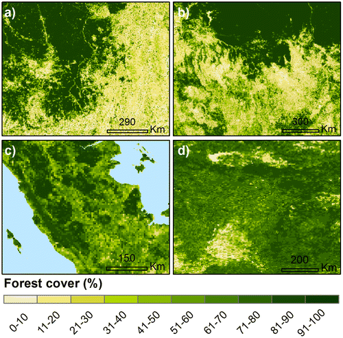
In addition to the above quantitative evaluation, visual inspection revealed that the integrated forest cover product depicted well-known patterns of forest cover across the globe (Figure 3). At 5-km resolution, a resolution that is too coarse to derive accurate area estimate (Hansen, Stehman, and Potapov 2010; Hansen et al. 2008; Mayaux and Lambin 1995), broad-scale forest cover patterns are clearly delineated, even in complex landscapes (Figure 4). Figure 4(a) focused on central Mato Grosso, Brazil, a transition region from humid Amazonian forests in the west to semi-arid Cerrado biome in the east. Located in the middle of the arc of deforestation, fragmented forest patches as a result of extensive human clearing are also clearly shown. Figure 4(b) showed the decreasing gradient of forest cover density from closed-canopy Congolese rainforests to woody savannas in southern Democratic Republic of the Congo. Figure 4(c) highlighted the difference of forest cover between primary forests (dark green patches) and oil palm plantations (light green patches) that replaced natural forests in Sumatra, Indonesia. Figure 4(d) shows the moderate-to-high density temperate/boreal forests along the border between China and Russia, where forests are subject to frequent logging activities and wildfires.

Figure 3. The integrated global forest cover map at 5-km spatial resolution.

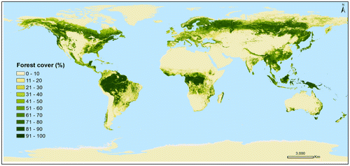
Figure 4. Regional details of the integrated forest cover map.

Notes: (a) Fragmented forest patches in northern Mato Grosso, Brazil centered at (52.746°W, 10.155°S). (b) Transition from forest to woody savanna in southern Democratic Republic of the Congo centered at (21.589°E, 6.185°S). (c) Primary forests and plantation forests in central Sumatra Island, Indonesia centered at (102.65°E, 1.686°S). (d) Moderate-to-high density temperate/boreal forests along China and Russia border, centered at (129.484°E, 52.167°N).

4. Discussion

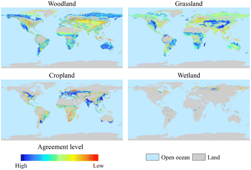
Extending a previous study, this paper has applied a data fusion approach for improving global forest cover mapping. However, forests are one of the most easily distinguished vegetation types using remotely sensed data (Hansen and Loveland 2012). Other forms of vegetative land cover such as woodland, grassland, cropland, and wetland show similar, if not necessarily larger, magnitude of discrepancies among different global land cover products (Figure 5). Existing studies on land cover data integration mainly focused on either forest (Schepaschenko et al. 2011, 2015; Song et al. 2014) or cropland (Fritz et al. 2011, 2015; Waldner et al. 2016), whereas studies rarely exist for improving global-scale woodland, grassland or wetland mapping. Accurately characterizing woodland and grassland is important not only for understanding the global carbon cycle (Poulter et al. 2014), but also for understanding agricultural production systems, as the world’s livestock are mainly produced on pasture land. Wetlands arguably have the largest monetary value in terms of the ecosystem goods and services that they provide to human society (Costanza et al. 2014). However, wetlands appear to be the most poorly mapped land cover at the global scale. The type- and scale-invariant feature of our developed data integration approach may be applied to these major vegetative land cover types. The first step is to understand where and why discrepancies occur (Figure 5). Creating spatially explicit presentation of agreement data using independent products not only reveals the persistent challenges of land cover mapping (that is, disagreement regions) but also provides a cost-effective way of selecting reliable training (agreement regions) for new land cover product generation (Zhang et al. in review). Potential issues of implementation include to reconcile various definitions of land cover and to collect sufficient regional high-quality data for reference. Evaluating the feasibility of method is a subject of our future research.

Figure 5. Agreement and disagreement of global land cover maps for woodland, grassland, cropland, and wetland.

5. Conclusions

Global-scale land cover characterization features persistent challenges regardless of the increasing spatial resolution. Data fusion has been proved to be a viable means of improving land cover mapping. The machine learning-based data integration method we have developed provides a generic framework for synthesizing the knowledge of experts who focus on global-scale land cover mapping and the knowledge of experts who specialize in a specific region, while the latter can be used as reference to calibrate the former. The effectiveness of the approach was fully demonstrated in (Song et al. 2014) for North America and the global-scale application was shown in this paper. We expect the type- and scale-invariant nature of the method to be useful for improving global-scale characterization of other major land cover types such as cropland, woodland, grassland, and wetland in future research. The ensemble approach can also be internalized for improving data quality when generating a global land cover product, where multiple versions can be produced and subsequently integrated.

Funding

This study is a contribution to the Global Forest Cover Change project (http://glcf.umd.edu/data/landsatFCC/) funded by NASA’s Making Earth System Data Records for Use in Research Environments (MEaSUREs) Program [grant number NNX08AP33A]. Additional support is provided by the NASA Earth and Space Science Fellowship (NESSF) Program [grant number NNX12AN92H].

Notes on contributors

Xiao-Peng Song is a postdoctoral research associate at the Department of Geographical Sciences, University of Maryland, USA. He received his PhD in Geographical Sciences from University of Maryland, BSc in Geographic Information System, and BSc in Economics (double major) from Peking University, China. His research interests focus on mapping and monitoring land cover and land use change at local to global scales. He is also a recipient of the NASA Earth and Space Science Fellowship.

Chengquan Huang is a research professor at the Department of Geographical Sciences, University of Maryland, USA. He received his PhD in Geography from University of Maryland, MSc in Environmental Sciences, and BSc in Geology from Peking University, China. He is leading efforts to quantify forest change at national to global scales using Landsat data, and is developing approaches for mapping forest structure and biomass change by integrating field inventory data, airborne or space borne lidar, and Landsat derived forest disturbance history.

John R. Townshend is a Research Professor/Emeritus Professor at the Department of Geographical Sciences, University of Maryland, USA. He received his PhD and BSc in Geography from University College London, UK. His current research focuses on the rates and causes of vegetation cover change, especially deforestation, through the use of remotely sensed data from satellites. He is the director of the Global Land Cover Facility, which houses the largest open access non-governmental online collection of Landsat data in the world. He is also former Chair of the Department of Geographical Sciences and Dean of the College of Behavioral and Social Sciences, University of Maryland.

References

- Bartholomé, E., and A. S. Belward. 2005. “GLC2000: A New Approach to Global Land Cover Mapping from Earth Observation Data.” International Journal of Remote Sensing 26 (9): 1959–1977. doi:10.1080/01431160412331291297.
- Bicheron, P., P. Defourny, C. Brockmann, L. Schouten, C. Vancutsem, M. Huc, S. Bontemps, et al. 2008. GlobCover: Products Description and Validation Report. Toulouse Cedex, France: MEDIAS-France.
- Bonan, G. B. 2008. “Forests and Climate Change: Forcings, Feedbacks, and the Climate Benefits of Forests.” Science 320 (5882): 1444–1449. doi:10.1126/science.1155121.
- Bonan, G. B., S. Levis, L. Kergoat, and W. K. Oleson. 2002. “Landscapes as Patches of Plant Functional Types: An Integrating Concept for Climate and Ecosystem Models.” Global Biogeochemical Cycles 16 (2): 5. doi:10.1029/2000gb001360.
- Bossard, M., J. Feranec, and J. Otahel. 2000. CORINE Land Cover Technical Guide − Addendum 2000 (Technical Report). Copenhagen, Denmark: European Environment Agency.
- Chen, J., J. Chen, A. Liao, X. Cao, L. Chen, X. Chen, C. He, et al. 2014. “Global Land Cover Mapping at 30 m Resolution: A POK-based Operational Approach.” ISPRS Journal of Photogrammetry and Remote Sensing 103: 7–27. doi:10.1016/j.isprsjprs.2014.09.002.
- Costanza, R., R. de Groot, P. Sutton, S. van der Ploeg, S. J. Anderson, I. Kubiszewski, S. Farber, and R. K. Turner. 2014. “Changes in the Global Value of Ecosystem Services.” Global Environmental Change 26: 152–158. doi:10.1016/j.gloenvcha.2014.04.002.
- Danko, D. M. 1992. “The Digital Chart of the World Project.” Photogrammetric Engineering and Remote Sensing 58 (8): 1125–1128.
- Di Gregorio, A., and L. J. M. Jansen. 2005. Land Cover Classification System: Classification Concepts and User Manual: LCCS (Software Version 2). Rome, Italy: Food & Agriculture Org. http://www.fao.org/docrep/008/y7220e/y7220e00.htm
- DiMiceli, C. M., M. L. Carroll, R. A. Sohlberg, C. Huang, M. C. Hansen, and J. R. G. Townshend. 2011. Annual Global Automated MODIS Vegetation Continuous Fields (MOD44B) at 250 M Spatial Resolution for Data Years Beginning Day 65, 2000–2010, Collection 5 Percent Tree Cover. In University of Maryland, The Global Land Cover Facility. Accessed December 12, 2013. http://glcf.umd.edu/data/vcf/
- Fairbanks, D. H. K., M. W. Thompson, D. E. Vink, T. S. Newby, H. M. Van den Berg, and D. A. Everard. 2000. “South African Land-cover Characteristics Database: A Synopsis of the Landscape.” South African Journal of Science 96 (2): 69–82.
- Foley, J. A., R. Defries, G. P. Asner, C. Barford, G. Bonan, S. R. Carpenter, F. S. Chapin, et al. 2005. “Global Consequences of Land Use.” Science 309 (5734): 570–574. doi:10.1126/science.1111772.
- Friedl, M. A., D. K. McIver, J. C. F. Hodges, X. Y. Zhang, D. Muchoney, A. H. Strahler, C. E. Woodcock, et al. 2002. “Global Land Cover Mapping from MODIS: Algorithms and Early Results.” Remote Sensing of Environment 83: 287–302.10.1016/S0034-4257(02)00078-0
- Friedl, M. A., D. Sulla-Menashe, B. Tan, A. Schneider, N. Ramankutty, A. Sibley, and X. Huang. 2010. “MODIS Collection 5 Global Land Cover: Algorithm Refinements and Characterization of New Datasets.” Remote Sensing of Environment 114 (1): 168–182. doi:10.1016/j.rse.2009.08.016.
- Fritz, S., L. You, A. Bun, L. See, I. McCallum, C. Schill, C. Perger, J. Liu, M. Hansen, and M. Obersteiner. 2011. “Cropland for Sub-Saharan Africa: A Synergistic Approach Using Five Land Cover Data Sets.” Geophysical Research Letters 38 (4): L04404. doi:10.1029/2010gl046213.
- Fritz, S., L. See, I. McCallum, L. You, A. Bun, E. Moltchanova, M. Duerauer, et al. 2015. “Mapping Global Cropland and Field Size.” Global Change Biology 21: 1980–1992. doi:10.1111/gcb.12838.
- Giri, C., B. Pengra, J. Long, and T. R. Loveland. 2013. “Next Generation of Global Land Cover Characterization, Mapping, and Monitoring.” International Journal of Applied Earth Observation and Geoinformation 25: 30–37. doi:10.1016/j.jag.2013.03.005.
- Gong, P., J. Wang, L. Yu, Y. Zhao, Y. Zhao, L. Liang, Z. Niu, et al. 2013. “Finer Resolution Observation and Monitoring of Global Land Cover: First Mapping Results with Landsat TM and ETM+ Data.” International Journal of Remote Sensing 34 (7): 2607–2654. doi:10.1080/01431161.2012.748992.
- Hansen, M. C., and T. R. Loveland. 2012. “A Review of Large Area Monitoring of Land Cover Change Using Landsat Data.” Remote Sensing of Environment 122: 66–74. doi:10.1016/j.rse.2011.08.024.
- Hansen, M. C., R. S. Defries, J. R. G. Townshend, and R. A. Sohlberg. 2000. “Global Land Cover Classification at 1 km Spatial Resolution Using a Classification Tree Approach.” International Journal of Remote Sensing 21 (6–7): 1331–1364.10.1080/014311600210209
- Hansen, M. C., R. S. DeFries, J. R. G. Townshend, M. Carroll, C. Dimiceli, and R. A. Sohlberg. 2003. “Global Percent Tree Cover at a Spatial Resolution of 500 Meters: First Results of the MODIS Vegetation Continuous Fields Algorithm.” Earth Interactions 7 (10): 1–15.10.1175/1087-3562(2003)007<0001:GPTCAA>2.0.CO;2
- Hansen, M. C., S. V. Stehman, P. V. Potapov, T. R. Loveland, J. R. Townshend, R. S. DeFries, K. W. Pittman, et al. 2008. “Humid Tropical Forest Clearing from 2000 to 2005 Quantified by Using Multitemporal and Multiresolution Remotely Sensed Data.” Proceedings of the National Academy of Sciences 105 (27): 9439–9444. doi:10.1073/pnas.0804042105.
- Hansen, M. C., S. V. Stehman, and P. V. Potapov. 2010. “Quantification of Global Gross Forest Cover Loss.” Proceedings of the National Academy of Sciences 107 (19): 8650–8655. doi:10.1073/pnas.0912668107.
- Hansen, M. C., P. V. Potapov, R. Moore, M. Hancher, S. A. Turubanova, A. Tyukavina, D. Thau, et al. 2013. “High-resolution Global Maps of 21st-Century Forest Cover Change.” Science 342: 850–853. doi:10.1126/science.1244693.
- Homer, C., C. Huang, L. Yang, B. Wylie, and M. Coan. 2004. “Development of a 2001 National Land-cover Database for the United States.” Photogrammetric Engineering & Remote Sensing 70 (7): 829–840.10.14358/PERS.70.7.829
- Huang, C., S. Kim, K. Song, J. R. G. Townshend, P. Davis, A. Altstatt, O. Rodas, et al. 2009. “Assessment of Paraguay’s Forest Cover Change Using Landsat Observations.” Global and Planetary Change 67 (1–2): 1–12. doi:10.1016/j.gloplacha.2008.12.009.
- Jung, M., K. Henkel, M. Herold, and G. Churkina. 2006. “Exploiting Synergies of Global Land Cover Products for Carbon Cycle Modeling.” Remote Sensing of Environment 101 (4): 534–553. doi:10.1016/j.rse.2006.01.020.
- Kim, H., J. O. Sexton, P. Noojipady, C. Huang, A. Anand, S. Channan, M. Feng, and J. R. Townshend. 2014. “Global, Landsat-based Forest-cover Change from 1990 to 2000.” Remote Sensing of Environment 155: 178–193. doi:10.1016/j.rse.2014.08.017.
- Latham, J., R. Cumani, I. Rosati, and M. Bloise. 2014. Global Land Cover Share (GLC-SHARE) Database Beta-release Version 1.0-2014. Rome: Food and Agriculture Organization. http://www.glcn.org/databases/lc_glcshare_en.jsp
- Liu, J., M. Liu, X. Deng, D. Zhuang, Z. Zhang, and D. Luo. 2002. “The Land Use and Land Cover Change Database and its Relative Studies in China.” Journal of Geographical Sciences 12 (3): 275–282.
- Loveland, T. R., B. C. Reed, J. F. Brown, D. O. Ohlen, Z. Zhu, L. Yang, and J. W. Merchant. 2000. “Development of a Global Land Cover Characteristics Database and IGBP DISCover from 1 km AVHRR Data.” International Journal of Remote Sensing 21 (6–7): 1303–1330. doi:10.1080/014311600210191.
- Mayaux, P., and E. F. Lambin. 1995. “Estimation of Tropical Forest Area from Coarse Spatial Resolution Data: A Two-step Correction Function for Proportional Errors due to Spatial Aggregation.” Remote Sensing of Environment 53: 1–15.10.1016/0034-4257(95)00038-3
- Montesano, P. M., R. Nelson, G. Sun, H. Margolis, A. Kerber, and K. J. Ranson. 2009. “MODIS Tree Cover Validation for the Circumpolar Taiga–Tundra Transition Zone.” Remote Sensing of Environment 113 (10): 2130–2141. doi:10.1016/j.rse.2009.05.021.
- Myneni, R. B., S. Hoffman, Y. Knyazikhin, J. L. Privette, J. Glassy, Y. Tian, Y. Wang, et al. 2002. “Global Products of Vegetation Leaf Area and Fraction Absorbed PAR from Year One of MODIS Data.” Remote Sensing of Environment 83 (1–2): 214–231. doi:10.1016/S0034-4257(02)00074-3.
- Olson, J. S. 1994. Global Ecosystem Framework-definitions (Internal Report). Sioux Falls, SD: USGS EROS Data Center. http://scholar.google.com/scholar_lookup?title=Global+ecosystem+framework-definitions&author=J.+Olson&publication_year=1994
- Pan, Y., R. A. Birdsey, J. Fang, R. Houghton, P. E. Kauppi, W. A. Kurz, O. L. Phillips, et al. 2011. “A Large and Persistent Carbon Sink in the World’s Forests.” Science 333 (6045): 988–993. doi:10.1126/science.1201609.
- Pflugmacher, D., O. N. Krankina, W. B. Cohen, M. A. Friedl, D. Sulla-Menashe, R. E. Kennedy, P. Nelson, et al. 2011. “Comparison and Assessment of Coarse Resolution Land Cover Maps for Northern Eurasia.” Remote Sensing of Environment 115 (12): 3539–3553. doi:10.1016/j.rse.2011.08.016.
- Pimm, S. L., C. N. Jenkins, R. Abell, T. M. Brooks, J. L. Gittleman, L. N. Joppa, P. H. Raven, C. M. Roberts, and J. O. Sexton. 2014. “The Biodiversity of Species and Their Rates of Extinction, Distribution, and Protection.” Science 344 (6187): 1246752. doi:10.1126/science.1246752.
- Potapov, P., S. Turubanova, and M. C. Hansen. 2011. “Regional-Scale Boreal Forest Cover and Change Mapping Using Landsat Data Composites for European Russia.” Remote Sensing of Environment 115 (2): 548–561. doi:10.1016/j.rse.2010.10.001.
- Potapov, P. V., S. A. Turubanova, M. C. Hansen, B. Adusei, M. Broich, A. Altstatt, L. Mane, and O. Justice. 2012. “Quantifying Forest Cover Loss in Democratic Republic of the Congo, 2000–2010, with Landsat ETM+ Data.” Remote Sensing of Environment 122: 106–116. doi:10.1016/j.rse.2011.08.027.
- Poulter, B., D. Frank, P. Ciais, R. B. Myneni, N. Andela, J. Bi, G. Broquet, et al. 2014. “Contribution of Semi-arid Ecosystems to Interannual Variability of the Global Carbon Cycle.” Nature 509 (7502): 600–603. doi:10.1038/nature13376.
- Running, S. W., T. R. Loveland, L. L. Pierce, R. R. Nemani, and E. R. Hunt Jr. 1995. “A Remote Sensing Based Vegetation Classification Logic for Global Land Cover Analysis.” Remote Sensing of Environment 51 (1): 39–48.10.1016/0034-4257(94)00063-S
- Schepaschenko, D., I. McCallum, A. Shvidenko, S. Fritz, F. Kraxner, and M. Obersteiner. 2011. “A New Hybrid Land Cover Dataset for Russia: A Methodology for Integrating Statistics, Remote Sensing and in Situ Information.” Journal of Land Use Science 6 (4): 245–259. doi:10.1080/1747423x.2010.511681.
- Schepaschenko, D., L. See, M. Lesiv, I. McCallum, S. Fritz, C. Salk, E. Moltchanova, et al. 2015. “Development of a Global Hybrid Forest Mask through the Synergy of Remote Sensing, Crowdsourcing and FAO Statistics.” Remote Sensing of Environment 162: 208–220. doi:10.1016/j.rse.2015.02.011.
- Sellers, P. J., Y. Mintz, Y. C. Sud, and A. Dalcher. 1986. “A Simple Biosphere Model (SIB) for Use within General Circulation Models.” Journal of the Atmospheric Sciences 43 (6): 505–531. doi:10.1175/1520-0469(1986)043<0505:asbmfu>2.0.co;2.
- Sexton, J. O., X. Song, M. Feng, P. Noojipady, A. Anand, C. Huang, D. Kim, et al. 2013. “Global, 30-m Resolution Continuous Fields of Tree Cover: Landsat-based Rescaling of MODIS Vegetation Continuous Fields with Lidar-based Estimates of Error.” International Journal of Digital Earth 6 (5): 427–548. doi:10.1080/17538947.2013.786146.
- Sexton, J. O., P. Noojipady, X. Song, M. Feng, D. Song, D. Kim, A. Anand, et al. 2016. “Conservation Policy and the Measurement of Forests.” Nature Climate Change 6 (2): 192–196. doi:10.1038/nclimate2816.
- Song, X., C. Huang, M. Feng, J. O. Sexton, S. Channan, and J. R. Townshend. 2014. “Integrating Global Land Cover Products for Improved Forest Cover Characterization: An Application in North America.” International Journal of Digital Earth 7 (9): 709–724. doi:10.1080/17538947.2013.856959.
- Song, X. P., C. Huang, J. O. Channan, and J. R. Townshend. 2014. “Annual Detection of Forest Cover Loss Using Time Series Satellite Measurements of Percent Tree Cover.” Remote Sensing 6 (9): 8878–8903.10.3390/rs6098878
- Song, X., C. Huang, S. S. Saatchi, M. C. Hansen, and J. R. Townshend. 2015. “Annual Carbon Emissions from Deforestation in the Amazon Basin between 2000 and 2010.” PLoS ONE 10 (5): e0126754. doi:10.1371/journal.pone.0126754.
- Thackway, R., A. Lee, Randall Donohue, Rodney J. Keenan, and Mellissa Wood. 2007. “Vegetation Information for Improved Natural Resource Management in Australia.” Landscape and Urban Planning 79 (2): 127–136. doi:10.1016/j.landurbplan.2006.02.003.
- Townshend, J. R., J. G. Masek, C. Huang, E. F. Vermote, F. Gao, S. Channan, J. O. Sexton, et al. 2012. “Global Characterization and Monitoring of Forest Cover Using Landsat Data: Opportunities and Challenges.” International Journal of Digital Earth 5 (5): 373–397. doi:10.1080/17538947.2012.713190.
- Tsendbazar, N. E., S. de Bruin, and M. Herold. 2016. “Integrating Global Land Cover Datasets for Deriving User-specific Maps.” International Journal of Digital Earth 10 (3): 219–237. doi:10.1080/17538947.2016.1217942.
- Waldner, F., S. Fritz, A. Di Gregorio, D. Plotnikov, S. Bartalev, N. Kussul, P. Gong, et al. 2016. “A Unified Cropland Layer at 250 m for Global Agriculture Monitoring.” Data 1 (1): 3.10.3390/data1010003
- White, M. A., J. D. Shaw, and R. D. Ramsey. 2005. “Accuracy Assessment of the Vegetation Continuous Field Tree Cover Product Using 3954 Ground Plots in the South-Western USA.” International Journal of Remote Sensing 26 (12): 2699–2704. doi:10.1080/01431160500080626.
- Wulder, M. A., J. C. White, M. Cranny, R. J. Hall, J. E. Luther, A. Beaudoin, D. G. Goodenough, and J. A. Dechka. 2008. “Monitoring Canada’s Forests. Part 1: Completion of the EOSD Land Cover Project.” Canadian Journal of Remote Sensing 34 (6): 549–562.10.5589/m08-066
- Wulder, M. A., J. G. Masek, W. B. Cohen, T. R. Loveland, and C. E. Woodcock. 2012. “Opening the Archive: How Free Data Has Enabled the Science and Monitoring Promise of Landsat.” Remote Sensing of Environment 122: 2–10. doi:10.1016/j.rse.2012.01.010.
- Zhang, R., C. Huang, X. Zhan, H. Jin, and X. Song. in Review. “Development of S-NPP VIIRS Global Surface Type Classification Map Using Support Vector Machines.” International Journal of Digital Earth.