Routing through open spaces – A performance comparison of algorithms

Abstract

Finding the shortest path through open spaces is a well-known challenge for pedestrian routing engines. A common solution is routing on the open space boundary, which causes in most cases an unnecessarily long route. A possible alternative is to create a subgraph within the open space. This paper assesses this approach and investigates its implications for routing engines. A number of algorithms (Grid, Spider-Grid, Visibility, Delaunay, Voronoi, Skeleton) have been evaluated by four different criteria: (i) Number of additional created graph edges, (ii) additional graph creation time, (iii) route computation time, (iv) routing quality. We show that each algorithm has advantages and disadvantages depending on the use case. We identify the algorithms Visibility with a reduced number of edges in the subgraph and Spider-Grid with a large grid size to be a good compromise in many scenarios.

Keywords:

• OpenStreetMap
• routing
• open space
• navigation
• pedestrian
• polygon

1. Introduction

Nowadays, there are many available web services that offer various kinds of routing (e.g. car, bicycle, pedestrian). All the underlying routing engines work similarly: they convert a geographic data-set into a routing graph consisting of nodes and edges (Caldwell 1961). This works well for motorized vehicles (e.g. car, bus, truck, ), because they are restricted to move on linear features like paths, ways, roads, or streets. However, pedestrians and cyclists are also able to move on areal features.

We call these features open spaces. They can be squares, plazas, parks, or even beaches. Integrating these features into the routing graph requires sophisticated algorithms. Most of the routing engines use the quite trivial approach to integrate only the boundary of the open space into the routing graph. This can cause unnecessarily long routes with an unrealistic shape (Dzafic et al. 2015). A possible solution for this problem is to precompute subgraphs (virtual ways) within the open space (Dzafic et al. 2015; Graser 2016). This paper compares different algorithms that create these virtual ways. They are assessed by four different criteria: (i) additional number of edges in the graph, (ii) additional graph creation time, (iii) route computation time, (iv) route quality (average length of the produced routes). We focus our examinations to scenarios where the graph is optimized using contraction hierarchies (CH) (Geisberger et al. 2008) and the shortest way is computed using the Dijkstra algorithm (Dijkstra 1959).

2. Related work

Finding the shortest way through an open space with obstacles is a common problem in robotics. Masehian and Amin-Naseri (2004) described a method which is based on Visibility graphs and Voronoi diagrams.

Walter et al. (2006) presented a raster based approach for pedestrian routing. They generalized open spaces using a Skeleton algorithm. This enables routing through them. Elias (2007) also used a Skeleton algorithm but applied it to vector data. Haunert and Sester (2008) used a Skeleton algorithm for geographic generalization of roads which are modeled as areas. Their approach also makes it possible to do routing on open spaces. Similarly, Van Toll et al. (2011) presented an approach to create routing subgraphs using the Medial-Axis algorithm.

Krisp et al. (2010) compared two versions of the Visibility algorithm: Visibility graph and the Visibility polygon. In contrast to the algorithm tested in this paper, they used an areal representation of the street network as input data (no linear features). Hence, their findings have limited relevance for our research question.

Bauer et al. (2014) do not create a subgraph, but they find a route through an open space by postprocessing: if a computed route leads along an open space, the route will be changed in a way that it crosses the open space. Dzafic et al. (2015) proved that this approach can fail under certain circumstances: they showed that avoiding the open space may turn out to be shorterthan moving along its boundary. Hence, the computed route does not touch the open space. Consequently, it is not possible anymore to compute a shortcut through the open space. Dzafic et al. (2015) proposed to solve this problem by adding a Spider Grid subgraph within the open space. This guarantees that the routing engine initially finds routes through open spaces.

Andreev et al. (2015) investigated possibilities for pedestrian routing in general: they added sidewalks to streets and enabled routing through open spaces with obstacles. Their approach makes it possible to start or end a route on an open space. They use an improved Visibility algorithm that avoids creating unnecessary edges (i.e. edges that are never part of any routing scenario that crosses the open space). Their approach produces less than 30% additional edges.

Graser (2016) examined four open space algorithms (Medial Axis, Straight Skeleton, Grid, and Visibility). She concluded that Visibility is best suitable for open space routing because it finds the most realistic route. Like Andreev et al. (2015) she suggested an improved version of this algorithm. Olbricht (2016) also proposed a Visibility algorithm. He estimated that a routing graph would grow by around 20% if additional edges in open spaces are integrated. Indoor navigation also faces the problem of integrating open spaces. Liu and Zlatanova (2015) used a visibility graph, Xu et al. (2016) chose a Delaunay-based approach for routing within buildings.

In summary, we find, that most of the mentioned work focuses only on describing different algorithms. However, just a few (Andreev et al. 2015; Olbricht 2016) have investigated how a routing engine is affected by the implementation of these algorithms. This paper aims to fill this research gap.

3. Method

We implemented a couple of open space algorithms into the routing engine GraphHopper (www.graphhopper.com) and tested them with three different study sites.

3.1. Open space algorithms

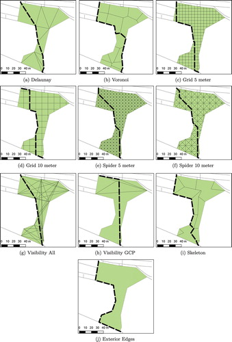
We chose the algorithms Grid, Spider-Grid, Visibility, Delaunay, Voronoi, and Skeleton for our analysis. Figure 1 shows an example of each algorithm. The Exterior Edge algorithm corresponds to the method to only integrate the boundaries of the open space. Grid and Spider are created with 5 and 10 m grid size, respectively. We chose two versions of the Visibility algorithm: the “Visibility All” algorithm connects all nodes of the surrounding polygon if there is direct a line-of-sight between them. This approach can lead to a lot of additional connections if the polygon has many nodes. Visibility Graph Connection Points (GCP) connects only the points of the surrounding polygon which have a node degree higher than two. Like in “Visibility All,” a connection is only created if a direct connection without obstacle is possible. The advantage of “Visibility GCP” is that it only connects nodes that are actually linked to other parts of the routing networks e.g. nodes that connect the open space with a road.

Figure 1. Routing examples using different algorithms (location: Weisenhausplatz, Pforzheim in Germany).

Notes: The gray lines within the open space show the subgraph of the respective algorithm. The black dotted line shows the shortest path from the top-left to the lower-right.

3.2. Study sites

For this analysis, we used the OpenStreetMap (OSM) data (date: 01 August 2016) from Austria, Baden-Württemberg (Germany) and Bavaria (Germany). These areas are comparably well mapped in OSM, and have a diverse landscape consisting of both big cities and rural areas. A study by Neis et al. (2012) shows that the OSM road data-set has a similar quality as a comparable commercial data-set. Hence, the tested data-sets should serve well as a model for other/bigger regions including e.g. whole Europe. Table 1 shows some statistical information about the study sites.

The analysis uses the pedestrian profile of GraphHopper. It excludes some open spaces that do not have the required tagging (e.g. access = no). Only open spaces stored as ways (closed linestrings) are considered. Open spaces that are stored as relations (multipolygons) are not considered because they are more difficult to process. Nevertheless, the analysis is still representative, since approximately 90% of the open spaces are stored as ways (shown by the OSM data-set statistics in Table 1).

3.3. Evaluation criteria

In order to evaluate the algorithms, we examined them according to the four criteria mentioned in the introduction.

The additional size of the graph and the graph creation time were both measured in the same experiment. We ran each algorithm for each study sites and measured the time and the count of created edges. These results were compared with the Exterior Edge algorithm that served as a base line. We measured the average route computation time for each algorithm using 18 route samples through urban areas in Baden-Württemberg. Each route has a linear distance of 10 km. The route samples do not necessary lead through an open space. However, the subgraphs in the open spaces still influence the routing performance, since the additional edges increase the size of the routing graph in the memory, which in turn increases the computation time of the routes. We measured the route quality by comparing the average length of the routing results through open spaces. We used 25 sample routes through open spaces (with different shapes) in Baden-Württemberg.

Like stated earlier, we focus our examinations to scenarios where the graph is optimized using contraction hierarchies (CH). This technique optimizes the routing graph by adding shortcuts to the underlying road network. The consequence is that routing requests can be handled much faster. Nevertheless creating CH requires additional time and storage (Geisberger et al. 2008). In order to better compare our results, we also computed the graph without the usage of CH.

4. Results

4.1. Graph size

Figure 2 shows the results if CH are used in the graph generation process. The diagram of Austria is ordered by additional edge count. For better comparability, the diagrams of the two other regions have the same order. The increase in the number of edges has a similar pattern among the three study sites. In Baden-Württemberg, the edge increase is higher than in Austria and Bavaria because it has a higher share of open spaces (cf. Table 1). We observed that even single open spaces may increase the graph size significantly. The edge count of Grid and Spider is dependent on the area – the edge count of the remaining algorithms is dependent on the node count of the input polygon. Hence, open spaces with large area or high node count have a big impact on the total edge count.

Table 2 shows the share of open spaces where the creation of the subgraphs has failed. In most cases, the reason is not an error in the respective implementation, but a normal consequence of the input parameters, e.g. the high “failure” number of Visibility GCP can easily be explained. Often there is no possibility that the existing GCPs of the input polygon can be connected with each other. This may happen if there is just one GCP or the existing GCPs are situated on the same line or there is no direct line-of-sight connection between the existing GCPs in the case of concave polygons. The failures of the Visibility All algorithm have the same reasons. It simply happens less likely. The failures of Delaunay happen if the input polygon has just three corners. The Voronoi algorithm always succeeds. The reasons for the failures of Grid are that the underlying polygon is smaller than the grid size of the algorithm. The Spider algorithm does not have this problem because it is always possible to fit the diagonals inside the input polygon. Malformed polygons (e.g. self-intersecting polygons, ) are the reasons for the few failures of the Spider algorithms. The few failures of the Skeleton algorithm are caused by the applied implementation (www.github.com/kendzi/kendzi-math/) and the properties (complexity, size, ) of the input polygons.

Table 1. Information about study site.

Criterion of comparison	Austria	Baden-Württemberg	Bavaria
Open spaces
Total	3267	5916	5362
Ways	2922	5409	4917
Relations	345	507	445
Processed ways	1889	4654	3372
OSM ways [million]	1.44	1.47	1.90
Created edges [million]	2.46	2.70	3.44
Share	0.23%	0.4%	0.28%

Notes: The top three rows show the total count of open spaces and how many of them are modeled as ways (closed linestrings) and relations (multipolygons). Row four shows the count of the open spaces that were actually processed in the analysis (using the pedestrian profile from GraphHopper). Rows five and six shows the count of ways tagged as “highway” and the count of resulting routing edges without the use of any open space algorithm. The last row shows the share of open spaces on the total count of “highway” ways.

Table 2. Share (%) of failed open space algorithms per test area.

Algorithm	Austria	Baden-Württemberg	Bavaria
Visibility GCP	26	25	31
Visibility All	1	1	1
Delaunay	1	1	1
Voronoi	0	0	0
Grid 5 m	1	1	1
Grid 10 m	4	4	4
Spider 5 m	0	0	0.1
Spider 10 m	0.1	0.1	0.1
Skeleton	1	1	1

Figure 2. Additional edge count and computation duration with usage of CH.

4.2. Graph creation time

The gray bars in Figures 2 and 3 show the additional computation time compared to the Exterior Edge algorithm. The usage of CH influences the result a lot. Consequently, two diagrams per region are displayed.

The first trivial observation is that higher edge count causes higher computation time. However, there is no linear dependency. The total computation time consists of both creating the graph edges and the CH post-processing. Figure 4 shows the absolute computation time with and without the computation of CH. This diagram visualizes how much more computation time is caused by the computation of CH.

There are two notable effects: (i) If Visibility All is applied, there is a lot of time need for the post-processing of the CH. We assume this is due to the fact that Visibility All creates many nodes with a lot of connections. This slows down the computation of the CH. (ii) The edge creation of Spider 5 m takes comparably long. The reason for this is that Spider 5 m needs to insert new nodes at the boundary of the polygon. This is computationally expensive.

Without the usage of CH (cf. Figure 3) the increase in computation time looks similar for the three test regions. The values of Baden-Württemberg are however higher because it has a higher share of open spaces. In contrast, the increase in computation time shows some differences if CH is used (cf. Figure 2): The increase in Visibility All in Austria and the increase in Spider 5 m in Baden-Württemberg is comparably high. We assume these effects are caused by the different characteristics (shape, complexity, size) of open spaces in each study site.

4.3. Routing performance

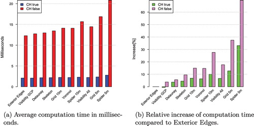
Figure 5(a) shows the average route computation time per algorithm. The ordering of the algorithms is the same as in the diagrams for the additional edge count and creation time of the graph (cf. Figure 2). In order to gain a reliable result, we computed each route 1000 times and used the average routing time. As expected, the computation with the use of CH is much faster than without.

The computation time within the algorithms varies a lot. Figure 5(b) shows the relative increase in computation time compared the common Exterior Edge algorithm which serves as a baseline. We observed that Visibility GCP may even be slightly faster than Exterior Edges when CH are used. A possible explanation for this behavior might be the characteristics of the Contraction Hierarchies algorithm. The relative increase in the computation time without the usage of CH is about two times higher than with CH.

Figure 6 shows that there is a linear dependence (cf. Pearson correlation coefficients inside the diagram) between the edge count and the routing performance. This may be explained by the fact that the larger the network is, the longer it takes to find the shortest path in it.

Overall, the increased computation time is still within an acceptable range. A normal user of a routing service will probably not notice if the computation time takes some milliseconds more. In contrast, a service provider who has to handle millions of requests per day might actually notice an increased resource consumption of the operating hardware.

Figure 3. Additional edge count and computation duration without the usage of CH.

Notes: (a) Austria, (b) Bavaria, (c) Baden-Württemberg

Figure 4. Comparison of graph generation times.

Notes: The percentage value on top of the green bars shows the share of the computation time without CH compared to the computation time with CH. (The computations have been run on a Quad-Core with 2.4 GHz).

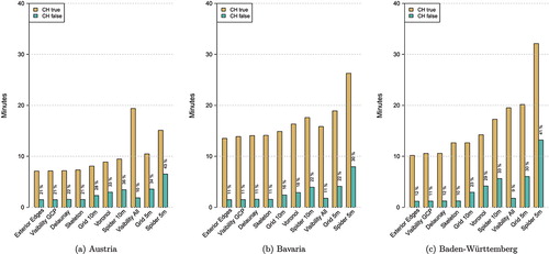
Figure 5. Routing performance.

Notes: (a) Average computation time in milliseconds. (b) Relative increase in computation time compared to Exterior Edges.

4.4. Routing quality

This analysis measures the quality of the algorithms by measuring its average length through 25 open spaces in Baden-Württemberg. Figure 1 gives a visual impression of the computed routes of one open space. Figure 7 shows how much longer the routes of each algorithm are compared to Visibility All. Visibility All delivers the shortest possible routes and serves as a reference for this statistics.

The Exterior Edges algorithm is around 50% longer. This is explained by the characteristic of this algorithm to not cross the open space at all but to always return routes along the boundary of the polygon. The average length of Visibility GCP is close to Visibility All. It generally shows good results, if the open space is convex because then a lot of connections can be created. If the open space has a rather concave shape, Visibility GCP has problems to create edges because often the direct line of sight is blocked. Both Spider algorithms deliver satisfying results in all cases. Please note that routes created with Spider 10 m are in average not much longer than routes produced with Spider 5 m. Delaunay delivers sufficient results. However, the results are varying. It is dependent on the configuration of the edges. Sometimes Delaunay even takes the optimal path, whereas it also happens that a very long path is chosen because the necessary routing edges are not available.

Both Grid algorithms produce routes that are around 20% longer than routes produced with Visibility All. Like the in the case of the Spider algorithms, it is remarkable that routes created with Grid 10 m are just slightly longer than routes created with Grid 5 m. The quality of the Grid algorithms depends on the orientation of the route. A roughly north–south or east–west oriented route leads to a satisfying routing quality. In contrast, other orientations (e.g. diagonal) usually deliver bad results.

Voronoi mostly finds suitable routes. They, however, have many unnecessary curves, which causes a longer way. Moreover, this causes a strange shape of the routes. Another observation is that the Voronoi subgraph has never a direct connection to the original nodes of the open space geometry. It always connects to the middle of an edge. Therefore the resulting route always needs to go along the boundary of the open space before it can actually enter the open space. Routes computed with the Skeleton algorithm can be very chaotic, due to shortcomings in the applied straight skeleton algorithm. The underlying routing graph sometimes has gaps which prevent a sufficient routing result. Therefore in some cases, it is shorter to stay on the boundary of the open space instead of using the Skeleton subgraph. Moreover – similar to Voronoi – many routes of Skeleton have a lot of unnecessary curves.

5. Comparison of algorithms

Table 3 summarizes our findings. Both the minimum and the maximum values of the results of the study sites are used. The colors (green, yellow, and red represent a good, medium, and bad result, respectively) indicate a rough qualitative assessment of the results depending on the “worst” result.

Spider and Grid are the only algorithms that properly handle routes which start or end inside of an open space. The biggest downside of the Grid algorithm is that it delivers poor results if the route is not north–south or east–west oriented. This effect may even not be solved by rotating the grid: a 45 rotated grid would, in turn, deliver bad results for north–south or east–west oriented routes. In contrast, the Spider algorithm always delivers good results, however, the graph size and the creation time might be very high.

The routing quality of Delaunay is varying: it is mostly good but produces sometimes poor results. However, according to the other criteria, Delaunay performs well. Voronoi delivers constant medium routing results. Additionally, the creation of the graph might take quite long as well. Therefore, it should be discouraged to use it in the current state. However, Voronoi might serve as a basis for developing a more advanced algorithm.

Our implementation of the Skeleton algorithm often delivers a subgraph that is not fully self-connected (i.e. gaps within the graph). Nevertheless, a few computed routes look quite promising. The routes” shapes look similar to the route that would be assumed to be chosen by humans crossing the square. Overall, the Skeleton algorithm in its current state has limited use for open space routing. There are however approaches how to improve it e.g. (Haunert and Sester 2008).

Visibility All performs perfectly in terms of the length of the resulting route. Nevertheless, it has the big downside, that the computation of the graph and particularly the post-processing of the CH might take very long. This is caused by the existence of nodes with high node degree, i.e. many connections to other nodes. In contrast, Visibility GCP can be computed quite fast. Its routing quality is mostly good, but sometimes (especially on concave open spaces) a few important connections are missing.

Figure 6. Edge count versus average routing time.

Figure 7. Increased route length compared to Visibility All.

Table 3. Algorithm comparison – usage of CH is considered.

6. Discussion

Our investigations are based on a modified version of the routing engine GraphHopper. Readers are reminded that this choice may have implications on the presented research findings. Furthermore, all our results are based on prototype versions of the described algorithms that may be subject to further optimization efforts. Therefore, the presented figures should be interpreted as a rough guideline for comparing the characteristics of the investigated algorithms.

In the following section, we want to critically assess some shortcomings of the chosen method and its results in detail:

We integrated only open spaces that are modeled as closed linestrings (OSM ways). As stated already it would have been more complex to consider multipolygons (OSM relations) as well, because of their possibly complex data structure. The inclusion of multipolygons would cause a higher count of (more complex) open spaces. This would increase the edge count of the routing graph and graph creation time. However, since the vast majority of the open spaces are modeled as closed linestrings (cf. Table 1), the respective increase would probably not be too high. In contrast, the presented open space algorithms could show a different performance (graph computation time and route computation time), if they have to handle more complex geometries of the multipolygon open spaces.

Sometimes, it happens that there are adjacent open spaces. The current approach computes a subgraph for each of these adjacent polygons. These subgraphs might not properly be connected to adjacent subgraphs. Olbricht (2016) suggests to solve this problem by merging adjacent open spaces. Hence, only one subgraph (instead of many subgraphs) would be computed. The additional implementation of this approach would probably cause different results for the examined research questions. Nevertheless, since adjacent open spaces are rare, we would expect only a slight change of the results.

As described in this paper, there are a couple of different possible algorithms for creating subgraphs in open spaces. Moreover, each of these algorithms can be modified (e.g. Visibility All and Visibility GCP), improved (e.g. Spider is an improved Grid algorithm) or can have different parameters (e.g. different grid size of Spider and Grid). This results in a very high number of possible open space algorithms. In this paper, we have only tested a few of them.

Some of our implementations of the algorithms suffer from (minor) shortcomings, e.g. handling of adjacent open spaces, unexpected holes in skeleton algorithm. Nevertheless, the basic versions of the most common open space algorithms were examined. The results provide an overview of the basic characteristics of each type of open space algorithm. Thus the findings of this paper can be transferred to similar open space algorithms and can furthermore contribute to the improvement of existing open space algorithms.

The quality assessment of the algorithms only takes the length of the computed algorithms into account. However, also other factors could be considered. The count of turns needed to cross the open space could be used: fewer turns would lead to simpler routing instructions. Moreover, the routing quality could be examined by the similarity to routes chosen by humans.

For the scope of this paper, we have used Austria, Baden-Württemberg and Bavaria as study sites. These regions are well mapped and have a diverse landscape and the results should, therefore, be transferable to other and also bigger regions (e.g. continents, global). In order to validate this, it would be necessary to rerun the whole analysis with a larger test area (e.g. Europe).

7. Conclusions and outlook

We have presented a comparison of different open space algorithms with regard to different optimization parameters. While none of the examined algorithms is an optimal solution for all considered parameters, each of them has advantages and disadvantages depending on the scenario. According to our results, the Visibility algorithms and the Spider algorithm seem to be most promising, however, they still require some optimization.

Visibility All creates too many unnecessary edges, while Visibility GCP misses edges that would actually be required for the optimal solution. Thus, a compromise between these algorithms would be desired: the result would be a visibility-based algorithm that has fewer edges than Visibility All and more edges than Visibility GCP. Graser (2016) and Andreev et al. (2015) suggest a possible solution for this purpose.

The Spider algorithm delivers routes that are close to the shortest route for many different cases. A big advantage is that this algorithm also interpolates nodes within the open space making it possible to define start and end points also in the open space. However, this comes at the cost of long graph creation times and a considerable increase in the graph size. In order to keep the graph size low, the subgraph of big open spaces could be computed with a bigger grid size. The choice of the grid size of the Spider algorithm is a trade-off between graph size and graph generation time and the possible routing quality.

Besides the choice of the algorithm, there are also other potential optimizations possible: the creation of a subgraph can be costly if the open space has many nodes. Therefore, it might be useful to perform a generalization of the polygon in order to simplify the computation of the (sub-)graph.

Recently, a Visibility algorithm has been implemented into a new version of the route planning service OpenRouteService (www.openrouteservice.org) (Schmitz et al. 2008), since this optimization is particularly useful for the pedestrian and wheelchair route planning profiles (Neis and Zielstra 2014; Neis 2015; Zipf et al. 2016; Hahmann et al. 2016).

Another possible use case of open space algorithms could also be to enhance a road data-set itself with additional edges, which would be an option to easily integrate the presented approach into a variety of different routing engines, without the need for re-implementation of the algorithms in each engine.

Integrating open spaces into a routing engine may also contribute to the improvement of the quality of the OSM data-set: it is easier to evaluate if an open space is properly connected to the street network by looking at the resulting routes through the open spaces. Moreover, OSM contains a lot of virtual paths within open spaces. Their only purpose is to help routing engines to find better routes through open spaces. The availability of an open space aware routing engine would make these paths obsolete. Hence, they could then be removed.

Notes on contributors

Stefan Hahmannis a Postdoc Researcher at Fraunhofer IVI, Institute for Transportation and Infrastructure, Dresden, where his main research interests are logistics during mass emergency and protection of critical infrastructure. Before, he has worked at Heidelberg University in the field of route planning and volunteered geographic information and as developer for Web-GIS at mapchart GmbH (Dresden). He has received a PhD degree from Technical University of Dresden in Geographic Information Science and studied Geodesy at the University of Applied Sciences, Dresden.

Jakob Mikschis a Research Assistant at the GIScience research group at Heidelberg University. He studied “Applied Geoinformatics” (M.Sc.) at the University of Salzburg and “Geography” (B.Sc.) at the University of Innsbruck. His research interests are route planning and spatial analysis.

Bernd Reschis an Assistant Professor at University of Salzburg’s Department of Geoinformatics - Z_GIS and a Visiting Fellow at Harvard University (USA). His research interests revolve around fusing data from human and technical sensors, including the analysis of social media. Amongst a variety of other functions, Bernd Resch is Editorial Board Member of the International Journal of Health Geographics, Associated Faculty Member of the doctoral college "GIScience", and Executive Board member of Spatial Services GmbH.

Johannes Lauerworks at HERE GmbH & Co KG. Before that, he worked at GIScience research group at Heidelberg University, Department of Geography. He has a background in applied computer science and GIScience from Bonn University. Currently, he is a PhD candidate (supervisor: Prof. Dr. Alexander Zipf). His research interest is in analysis of movement and sensor data, route planning and volunteered geographic information.

Alexander Zipfis the professor and chair of GIScience (Geoinformatics) at Heidelberg University (Department of Geography) since late 2009. He is member of the Centre for Scientific Computing (IWR), the Heidelberg Center for Cultural Heritage and PI at the Heidelberg graduate school MathComp. He is also founding member of the Heidelberg Center for the Environment (HCE). From 2012–2014 he was Managing Director of the Department of Geography, Heidelberg University. In 2011–2012 he acted as Vice Dean of the Faculty for Chemistry and Geosciences, Heidelberg University. Since 2012 he is speaker of the graduate school CrowdAnalyser – Spatio-temporal Analysis of User-generated Content. He is also member of the editorial board of several further journals and organized a set of conferences and workshops. 2012–2015 he was regional editor of the ISI Journal “Transactions in GIS” (Wiley). Before coming to Heidelberg he led the Chair of Cartography at Bonn University and earlier was Professor for Applied Computer Science and Geoinformatics at the University of Applied Sciences in Mainz, Germany. He has a background in Mathematics and Geography from Heidelberg University and finished his PHD at the European Media Laboratory EML in Heidelberg where he was the first PhD student. There he also conducted further research as a PostDoc for 3 years.

Additional information

Funding

This work was supported by European Commission [grant number 612096 (CAP4Access)].

References

- Andreev, S. , J. Dibbelt , M. Nöllenburg , T. Pajor , and D. Wagner . 2015. “Towards Realistic Pedestrian Route Planning.” In 15th Workshop on Algorithmic Approaches for Transportation Modelling, Optimization, and Systems (ATMOS 2015) , edited by G. F. Italiano and M. Schmidt , 48, 1–15. OpenAccess Series in Informatics (OASIcs), Dagstuhl: Schloss Dagstuhl-Leibniz-Zentrum fuer Informatik. doi:10.4230/OASIcs.ATMOS.2015.1.
- Bauer, C. , A. Amler , S. Ladstätter , and P. M. Luley . 2014. “Optimierte Wegefindung Fug\"{a}nger basierend auf vorhandenen OpenStreetMap-Daten.” [Optimized wayfinding for pedestrians based on OpenStreetMap-Data] Symposium für Angewandte Geoinformatik (AGIT), Salzburg, Österreich, July 2--4, 408–413.
- Caldwell, T. 1961. “On Finding Minimum Routes in a Network with Turn Penalties.” Communcaions ACM (New York, NY, USA) 4 (2 February): 107–108. doi:10.1145/366105.366184.
- Dijkstra, E. W. 1959. “A Note on Two Problems in Connexion with Graphs.” Numerische Mathematik 1 (1): 269–271.
- Dzafic, D. , S. Klug , D. Franke , and S. Kowalewski . 2015. “Routing über Flächen mit Spider WebGraph.” [Routing through open spaces using Spider WebGraph] Symposium für Angewandte Geoinformatik (AGIT), Salzburg, Österreich, July 8--10, 516–525.
- Elias, B. 2007. “Pedestrian Navigation -- Creating a Tailored Geodatabase for Routing.” 2007 4th Workshop on Positioning, Navigation and Communication, Hannover, Germany, March 22, 41–47. doi:10.1109/WPNC.2007.353611.
- Geisberger, R. , P. Sanders , D. Schultes , and D. Delling . 2008. “Contraction Hierarchies: Faster and Simpler Hierarchical Routing in Road Networks.” In Experimental Algorithms: 7th International Workshop, WEA 2008 Provincetown, MA, May 30--June 1, 2008 Proceedings, edited by C. C. McGeoch , 319–333. doi:10.1007/978-3-540-68552-424.
- Graser, A. 2016. “Integrating Open Spaces into OpenStreetMap Routing Graphs for Realistic Crossing Behaviour in Pedestrian Navigation.” GI\_Forum -- Journal for Geographic Information Science, Salzburg, Österreich, July 5--8 217–230.
- Hahmann, S. , A. Zipf , A. Rousell , A. Mobasheri , L. Loos , M. Rylov , E. Steiger , and J. Lauer . 2016. “GIS-Werkzeuge zur Verbesserung der barrierefreien Routenplanung aus dem Projekt CAP4Access.” [GIS-Tools to improve accessible route planning from the project CAP4Access] AGIT Journal für Angewandte Geoinformatik, Salzburg, Österreich, July 6--8.
- Haunert, J.-H. , and M. Sester . 2008. “Area Collapse and Road Centerlines based on Straight Skeletons.” GeoInformatica 12 (2): 169–191. doi:10.1007/s10707-007-0028-x.
- Krisp, J. , L. Lui , and T. Berger . 2010. “Goal Directed Visibility Polygon Routing for Pedestrian Navigation.” 7th International Symposium on LBS \ & TeleCartography, Guangzhou, China, September 20--22.
- Liu, L. , and S. Zlatanova . 2015. “An Approach for Indoor Path Computation Among Obstacles that Considers User Dimension.” ISPRS International Journal of Geo-Information 4 (4): 2821–2841. doi:10.3390/ijgi4042821.
- Masehian, E. , and M. R. Amin-Naseri . 2004. “A Voronoi Diagram-visibility Graph-potential Field Compound Algorithm for Robot Path Planning.” Journal of Robotic Systems 21 (6): 275–300. doi:10.1002/rob.20014.
- Neis, P. 2015. “Measuring the Reliability of Wheelchair User Route Planning based on Volunteered Geographic Information.” Transactions in GIS 19 (2): 188–201. doi:10.1111/tgis.12087.
- Neis, P. , and D. Zielstra . 2014. “Generation of a Tailored Routing Network for Disabled People Based on Collaboratively Collected Geodata.” Applied Geography 47 (Supplement C): 70–77.
- Neis, P. , D. Zielstra , and A. Zipf . 2012. “The Street Network Evolution of Crowdsourced Maps: OpenStreetMap in Germany 2007--2011.” Future Internet 4 (1): 1–21. doi:10.3390/fi4010001.
- Olbricht, R. 2016. “Braucht OpenStreetMap Flächen und Kanten?” Presentation. FOSSGIS Konferenz 2016, Salzburg, Austria, July 4--6. doi:10.5446/19725.
- Schmitz, S. , A. Zipf , and P. Neis . 2008. “New Applications Based on Collaborative Geodata -- The Case of Routing.” Proceedings of XXVIII INCA International Congress on Collaborative Mapping and Space Technology, Gandhinagar, Gujarat.
- Van Toll, W. , A. F. Cook , and R. Geraerts . 2011. “Navigation Meshes for Realistic Multi-layered Environments.” 2011 IEEE/RSJ International Conference on Intelligent Robots and Systems, San Francisco, CA, USA: IEEE, 3526–3532.
- Walter, V. , M. Kada , and H. Chen . 2006. “Shortest Path Analyses in Raster Maps for Pedestrian Navigation in Location Based Systems.” International Symposium on “Geospatial Databases for Sustainable Development”, Goa, India, ISPRS Technical Commission IV (on CDROM). Citeseer.
- Xu, M. , S. Wei , and S. Zlatanova . 2016. “An Indoor Navigation Approach Considering Obstacles and Space Subdivision of 2d Plan.” ISPRS -- International Archives of the Photogrammetry, Remote Sensing and Spatial Information Sciences (June): 339–346. doi:10.5194/isprs-archives-XLI-B4-339-2016.
- Zipf, A. , A. Mobasheri , A. Rousell , and S. Hahmann . 2016. “Crowdsourcing for Individual Needs -- The Case of Routing and Navigation for Mobility-impaired Persons.” In European Handbook of Crowdsourced Geographic Information , edited by C. Capineri , M. Haklay , H. Huang , V. Antoniou , J. Kettunen , F. Ostermann , and R. Purves , 325–337. London: Ubiquity Press.