Log-cumulants of the finite mixture model and their application to statistical analysis of fully polarimetric UAVSAR data

Abstract

Since its first flight in 2007, the UAVSAR instrument of NASA has acquired a large number of fully Polarimetric SAR (PolSAR) data in very high spatial resolution. It is possible to observe small spatial features in this type of data, offering the opportunity to explore structures in the images. In general, the structured scenes would present multimodal or spiky histograms. The finite mixture model has great advantages in modeling data with irregular histograms. In this paper, a type of important statistics called log-cumulants, which could be used to design parameter estimator or goodness-of-fit tests, are derived for the finite mixture model. They are compared with log-cumulants of the texture models. The results are adopted to UAVSAR data analysis to determine which model is better for different land types.

Keywords:

• Finite mixture model
• UAVSAR
• log-cumulant
• statistical analysis
• Polarimetric SAR (PolSAR)

1. Introduction

Unmanned Aerial Vehicles (UAVs) provide a fast, flexible, and low-cost solution to remote sensing. In the recent developments, different sensors including the traditional optical cameras and multispectral imaging devices have been mounted on UAVs to perform various remote sensing tasks. For Synthetic Aperture Radar (SAR) sensors, the carrier is required to move at a steady speed in a consistent direction to obtain high-quality data. And there exist many crucial issues concerning precision control and navigation of the platform as well as miniaturizing of the SAR sensors (Wang et al. 2016). Although large challenges are posed in SAR data acquisition using UAVs, the Jet Propulsion Laboratory (JPL) has made great process recently by developing the UAVSAR instrument (Hensley et al. 2008).

UAVSAR is a pod-based L-band SAR for interferometric repeat-track observations. The radar is designed to be operable on a UAV, but was initially demonstrated on a NASA Gulfstream III aircraft in 2007. By designing the radar to be housed in an external unpressurized pod, it has the potential to be readily ported to other platforms such as the Predator or Global Hawk UAVs. The primary objective of the side-looking UAVSAR instrument is to accurately map crustal deformations associated with natural hazards, such as volcanoes and earthquakes. The radar is fully polarimetric, with several important radar characteristics listed in Table 1 (Hensley et al. 2008).

The UAVSAR system has acquired a huge amount of Polarimetric SAR (PolSAR) data in high spatial resolution, and we need design efficient algorithms to interpret them. Due to the coherent interference among received waves, SAR data usually presents a salt-and-pepper appearance known as speckle. Although the speckle is a real electromagnetic measure, from the point of view of an acquisition system, it is considered as noise since it cannot be predicted accurately and contaminates the measure of the reflectivity. The target information must be extracted from the statistics of the data, and an accurate statistical model becomes very important in various PolSAR applications.

Gaussian distributions for the radar returns have been frequently assumed when there are a large number of scatterers within each resolution cell (Chen, Wang, and Sato 2012; Lee et al. 2015). But many experiments show that targets in high resolution data may show non-gaussian behaviors (Lee et al. 1994; Frery et al. 1997). Currently there are two main ways to model the non-gaussianity of data: texture model (or product model) and finite mixture model. A texture model assumes that the radar return is a product of two independent components, the speckle and the texture. The former is supposed to follow a complex Gaussian distribution, whereas the latter is a positive random variable modeling the variation of the radar cross-section. A considerable research effort has been dedicated to investigate texture models for PolSAR data (Yueh et al. 1989; Lee et al. 1994; Frery et al. 1997; Freitas, Frery, and Correia 2005; Bombrun and Beaulieu 2008).

On the contrary, the finite mixture model describes combinations of various targets, each may give aspecific scattering mechanism. This makes sense in certain scenes such as urban areas which usually consist of coherent targets like houses and roads, as well as distributed targets like trees and grass. The backscattering from the urban area represents a combination of different scattering mechanisms. Especially in high resolution data, it is possible to observe much smaller spatial features, offering the opportunity to explore the structures in the images. For data with irregular histograms (e.g. multimodal, spiky), the finite mixture model is more accurate than a single distribution such as a texture model (Moser, Zerubia, and Serpico 2006; Krylov et al. 2008; Wang, Ainsworth, and Lee 2015).

Table 1. Key system parameters of the UAVSAR instrument.

Parameter	Value
Frequency	1.26 GHz
Chirp Bandwidth	80 MHz
Range Resolution	1.67 m
Azimuth Resolution	0.8 m
Swath Width	16 km
Incidence Angle	–65

To determine the actual distribution of the data correctly, some comparative statistics, as well as tools to visualize the fit of the models to data, are in need. The log-cumulants, also known as the Mellin Kind Statistics (MKS), can be used to accomplish this task (Nicolas 2002; Bombrun and Beaulieu 2008; Anfinsen and Eltoft 2011; Bombrun, Anfinsen, and Harant 2011). It is demonstrated that log-cumulants are of great value for the analysis of PolSAR data, and that they can be used to derive estimators for distribution parameters with low bias and variance. Log-cumulants of the texture models are studied by many researchers (Anfinsen and Eltoft 2011; Bombrun, Anfinsen, and Harant 2011; Deng and López-Martínez 2016; Deng, López-Martínez, and Varona 2016). However, there is little work done regarding to the finite mixture model. In this paper, log-cumulants of the finite mixture models will be derived, and a comparison with those of the texture models will be drawn. The results will be adopted to UAVSAR data analysis to see which model is better for different land types.

2. SAR polarimetry

PolSAR systems measure the properties of a distant target by detecting the change of the polarization state that the target induces to the incident wave. Let h represent the horizontal polarization and v the vertical polarization, then the target under observation can be characterized by four complex-valued scattering coefficients(1)

The matrix is generally referred to as scattering matrix (Lee and Pottier 2009). In many cases, it is more flexible to represent the scattering matrix as a vector which is known as scattering vector. When studying the statistical behavior of the PolSAR data, the scattering vector for a reciprocal target can be expressed as follows:(2)

Targets under observation are commonly situated in a dynamically changing environment and are subjected to spatial and temporal variations. Despite the radar system transmits a perfectly polarized wave, the wave scattered by the target is partially polarized (Cloude 2009). Such scatterers are called distributed targets. The analysis of this type of targets cannot be performed exactly by one target but a population of targets. More precisely, they are analyzed by introducing the concept of space and time varying stochastic processes, where the targets are described by the second order moments such as the polarimetric coherency or covariance matrices.

The covariance matrix is defined as the expectation of the outer product of the target vector with its transpose conjugate(3)

where and denote the transpose conjugate and conjugate, respectively, and is the expectation operator. In practice, the number of scattering vectors used to calculate the expectation is limited. Let L denote the number of samples to compute the average, the PolSAR data then can be represented by the so-called sample covariance matrix(4)

where is the -th scattering vector. The averaging is also called multilooking which can be employed to reduce the speckle of PolSAR data, with L referring to the number of looks. In this paper, the statistical properties of are mainly studied.

3. Log-cumulants of the finite mixture model

3.1. Finite mixture model

The heterogeneity that appears in PolSAR data may result from the mixture of different targets. For instance, from an urban area which usually consists of different objects like houses, trees, and roads, the backscattering is a combination of responses from different scatterers. The forest areas sometimes can be treated as a mixture of bright clutters, and dark ones, corresponding to the strong returns from the crowns of trees and the shadows behind them. To represent this type of data, a simple distribution would be inappropriate. Finite mixture models, instead, could achieve reasonable level of accuracy (Moser, Zerubia, and Serpico 2006; Krylov et al. 2008, 2013; Wang, Ainsworth, and Lee 2015; Anfinsen 2016).

Assume that the region under analysis can be modeled by a mixture of components, then the overall Probability Density Function (PDF) of the data can be written as a weighted sum of the probabilities of each component (Frühwirth-Schnatter 2006)(5)

where is a vector containing all the parameters of the distribution, and the mixing weights obey(6)

The parameters of this distribution consist of the number of components K, the weights and the distribution parameter of each component . Those parameters could be estimated jointly using the Expectation-Maximization algorithm (EM algorithm), with auto-merging and auto-splitting strategies.

There are many options for the distributions of the mixing components, but here we mainly focus on the mixture of Wishart distributed components, since the Wishart distribution is widely used in PolSAR data modeling (Goodman 1963; Lee, Mitchell, and Kwok 1994; Tough, Blacknell, and Quegan 1995; López-Martínez and Fabregas 2003; Alonso-González, López-Martínez, and Salembier 2012). For different mixing components in the same image, the number of looks L is supposed to be consistent. The PDF, therefore, can be written as(7)

where d is the dimension of the scattering vector, assembling all the covariance matrices, and is given by(8)

The intensity PDF of the ith channel, which is also a finite mixture, is found to be(9)

with indexing the ith diagonal element of the kth covariance matrix.

The most interesting property of a mixture density is that the shape of the density is extremely flexible. It may be multimodal, or even if it is unimodal, may exhibit considerable skewness or additional humps. For this reason, the finite mixture distributions offer a flexible way to describe rather heterogeneous data (Frühwirth-Schnatter 2006).

3.2. Log-cumulants

To test if a model is suitable for the data or not, some measurable statistics are required. Log-cumulants are of great value for the analysis of the sample covariance matrix (Anfinsen and Eltoft 2011). Define the Mellin kind characteristic function as the Mellin transform of the PDF (Anfinsen and Eltoft 2011)(10)

where represents the space of Hermitian positive definite matrices, then the v-th order log-moment and log-cumulant are given by(11)

where , called the Mellin kind characteristic function of the second kind. As a matter of fact, the log-moments (or log-cumulants) are the moments (or cumulants) of the random variable mapped at the logarithmic scale, so the rules between the moments and the cumulants also apply to the log-moments and the log-cumulants. For example, they can be related by the combinatorial version of Faà di Bruno’s formula, which shows that the log-cumulants are polynomials of the log-moments(12)

For the texture models, texture distributions from the Pearson family are widely studied as they could provide explicit expressions for the PDF of . Here we also confine ourselves to the Pearson distributions as listed in Table 2. The log-cumulants of the texture models are found to be (Anfinsen and Eltoft 2011; Bombrun, Anfinsen, and Harant 2011; Deng, López-Martínez, and Varona 2016)(13)

where are given in Table 2, and is the multivariate extension of the polygamma function, which can be expressed as follows(14)

From independent and identically distributed samples , the sample log-cumulants can be estimated using Faà di Bruno’s formula, where is the estimated log-moments(15)

with denoting the number of samples and the th sample covariance matrix. To determine if a model is applicable, we can compare the log-cumulants calculated from the PDF and those estimated from the sample data.

Table 2. Texture distributions and log-cumulants.

Texture distribution	Log-cumulants
Gamma
Inverse Gamma
Fisher
Beta
Beta Prime

Figure 1. Matrix variate log-cumulants of mixtures. (a) Mixture of two components. (b) Mixture of three components.

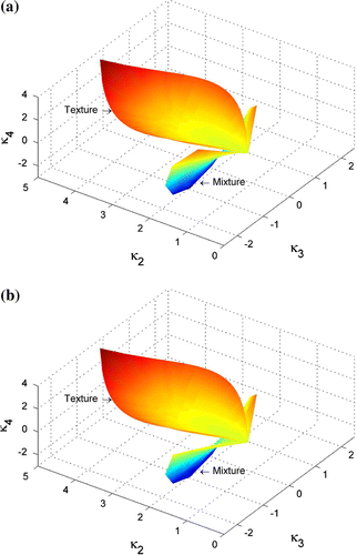
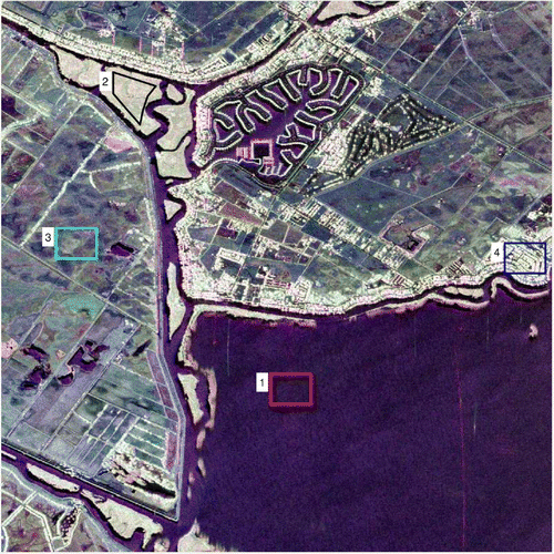
Figure 2. Pauli decomposition and ROIs of the first test site.

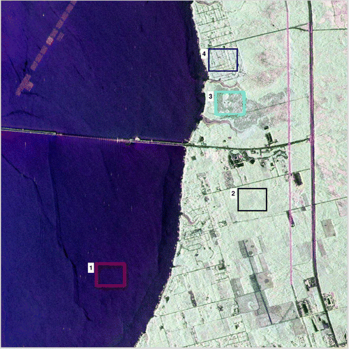
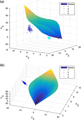
Figure 3. Log-cumulants estimated from different ROIs in the first test site. (a) One perspective of the 3D diagram. (b) Another perspective of the 3D diagram.

3.3. Log-cumulants of the finite mixture model

Inserting the PDF of the finite mixture model shown as Equation (7(7) ) into Equation (10(10) ), we have the Mellin kind characteristic function as(16)

Let denote the minimum determinant, that is , and , then the Mellin kind characteristic function can be reformulated as(17)

Write , by differentiating it v times with respect to s and then letting , the vth order log-cumulant is found to be(18)

It consists of three parts. The first part, , is due to the multilooking process, which mainly depends on the equivalent number of looks. This part is the same as that in texture models. The second part, denoted by , is the result from the mixture of targets. It can be solved recursively using(19)

where . Several examples of expanded expressions for are listed as follows:(20)

The relation between and is the same as that between log-cumulants and log-moments as illustrated by Equation (12(12) ). In fact, can be treated as the vth order log-moment of the ratios , and as the vth order log-cumulant, see Equations (12(12) ) and (15(15) ). The last part in Equation (18(18) ) depends on the minimum determinant of all covariance matrices. It vanishes when the order is larger than 1.

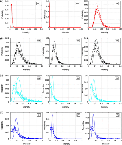
Figure 4. Histograms of the intensities from the first test site. (a) ROI 1. (b) ROI 2. (c) ROI 3. (d) ROI 4.

In the case of two mixing components, we have , and either or is equal to 1 according to their definition. Ignoring the subscript, can be written as , and the log-cumulants of the first several orders are(21)

Similarly, by representing the mixing weights corresponding to the non-minimum determinant as and , and the ratio of determinants to the minimum determinant as and (), the first four order log-cumulants of the mixture of three components can be calculated by(22)

By changing the mixing proportions through w and the ratios of determinants through , the log-cumulants of the finite mixture model could cover a wide range of values for each order. It has the same effect as by changing the texture distribution in the texture model. Generally, the second order (), the third order (), and the fourth order () are adopted to investigate the statistical properties of sample covariance matrices. Because the first order involves the determinant of covariance matrix, and higher orders (higher than 5, for example) require a large number of samples to get a low estimation variance (Deng and López-Martínez 2016).

By combining , , and together, we could discriminate various mixtures from textures. In Figure 1, log-cumulants of the above three orders are calculated from the texture models in Table 2 and plotted in a 3D diagram. Different values from 5 to 100 are tested for distribution parameters. It shows that these log-cumulants could make up a smooth surface. Log-cumulants of the same orders are also computed from mixtures of targets. Mixing proportions from 0 to 100%, and ratios of determinants from 1 to , are examined. When there exist mixing of two Wishart distributed components, the log-cumulants could also make up a smooth surface. When there are three components, the result is no longer a surface, a manifold instead. It is found that the log-cumulants of finite mixture models are always lying below those calculated from texture models.

As a matter of fact, the second order log-cumulant is proportional to the variance of a random variable, the third order to the skewness, and the fourth order to the kurtosis (excess kurtosis more exactly). This can be verified by expanding Faà di Bruno’s formula as expressed in Equation (12(12) ). When the variance and the skewness are equal, Figure 1 demonstrates that the finite mixture model could model data with smaller kurtosis than the texture models. In other words, the PDF of a finite mixture model has heavier or longer tails than those of texture models, since smaller kurtosis means less peaked in the PDF. In SAR or PolSAR data, heavy tails are very common (Sheen and Johnston 1992; Gini and Greco 2002; Lee and Pottier 2009), so the finite mixture model could provide a useful way to model this type of data.

4. Analysis of UAVSAR data

Two UAVSAR images downloaded from the website of Alaska Satellite Facility (ASF) are studied using the log-cumulants. The first test site is located at the West Panhandle of Florida, USA. Data in the multilook cross-product slant range format is analyzed, with number of looks in the range dimension and the azimuth dimension, respectively, equal to 3 and 12. The Equivalent Number of Looks (ENL) is estimated as 12.73 over a homogeneous sea area. This value is smaller than the product of the number of looks in the range and the azimuth dimensions due to the correlations between pixels. Pauli decomposition (Lee and Pottier 2009) is employed to illustrate the PolSAR data, with color coding:(23)

Four Regions Of Interest (ROI) covering land types in the sea area (ROI 1), the forest (ROI 2), the wetland (ROI 3), and the urban area (ROI 4), are analyzed, see Figure 2. Thanks to a high spatial resolution, each ROI contains pixels.

Log-cumulants of the second order, the third order and the fourth order are estimated from the four ROIs using the methods explained in Section 3.2. Since the sample size is not very large, we employ the bootstrap algorithm (Efron and Tibshirani 1994; Anfinsen and Eltoft 2011) to show the statistical behavior of the estimated values. Suppose there are N image pixels. The idea is to resample N times randomly, with replacement, from the original samples to build a new data-set called a bootstrap sample. Statistics are then computed from this bootstrap sample. By generating a large number, saying M, of independent bootstrap samples, we will obtain M estimated statistics, which can be used for further analysis like parameter estimation or visual presentation. The number of bootstrap samples, M, can be very large. In Figure 3, the estimated values from each bootstrap sample are represented by a “+” mark in the 3D diagram, and we have 100 bootstrap samples for each ROI.

Figure 5. Pauli decomposition and ROIs covering different land types of the second test site.

As a reference, log-cumulants of the same orders calculated from the texture models in Table 2 are also plotted. From the diagrams, we can see that different ROIs show different statistical behaviors. Specifically, the texture models are proper for the sea area and the forest area, while the finite mixture model makes a better representation than the texture models for the wetland area and the urban area, because the + clouds representing ROI 1 and ROI 2 are on the texture model surface, whereas those representing ROI 3 and ROI 4 are below it. More precisely, ROI 1 can be modeled by a Wishart distribution as the + cloud locate at the endpoint of the blue surface. Actually, the Pauli decomposition in Figure 2 shows that the first two ROIs are very homogeneous. ROI 3 and ROI 4, instead, consist of different targets. It can be seen that the log-cumulants estimated from ROI 3 are close to the surface in Figure 2. This may lead to a confusing statement that the region can be modeled by a texture model. To make more convincing conclusion, further methods such as goodness of fit are in need.

Figure 6. Log-cumulants estimated from different ROIs in the second test site. (a) Different perspective view of the 3D diagram. (b) Different perspective view of the 3D diagram. (c) Different perspective view of the 3D diagram.

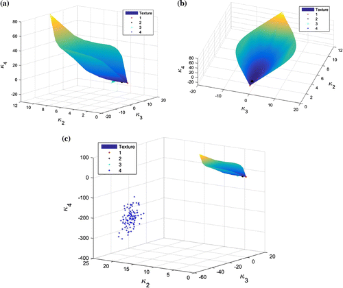
Figure 7. Histograms of the intensities from the second test site. (a) ROI 1. (b) ROI 2. (c) ROI 3. (d) ROI 4.

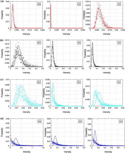
The histograms are also calculated for the intensity of each polarimetric channel, and they are compared with the PDFs of Gamma distributions, see Figure 4 where histograms are represented by dots and PDFs by solid lines. The first column in Figure 4 represents the HH channel, the second column represents the HV channel, and the last column represents the VV channel. Results from ROI 1 to ROI 4 are presented in row 1 to row 4. Here we choose the Gamma distributions as references because when the PolSAR data is Wishart distributed, the intensity of each individual channel should follow a Gamma distribution. The shape parameter of Gamma distributions is determined by the ENL, which is 12.73 for the test data as mentioned before. The scale parameter is estimated from data based on the mean value. Since the mean values are different, all the Gamma distributions have the same shape parameter but different scale parameters. From Figure 4, we can say that PolSAR data in the first ROI (red ROI 1) can be modeled by a Gaussian distribution, as the intensities of each polarimetric channel conform to the PDFs of Gamma distribution closely. While the other three regions show non-gaussian behavior. This confirms the observations using the log-cumulants.

However, there are several limits of histograms. First of all, the comparing results depend on the bin size of the histogram, and the comparison of PDFs is not effective. It is not easy to compare results across different experiments. In addition, this method usually exploits only the intensities of the data, regardless of the correlation between polarimetric channels. While for PolSAR data, this kind of correlation is very important in characterizing different targets. Finally, the difference between the finite mixture model and the texture models are not so easy to tell from histograms. This can be illustrated by the second row and the third row in Figure 4, where all the histograms seem to be unimodal, and quite different from the PDFs of Gamma distributions. With log-cumulants, we could avoid such problems.

The second image was acquired over Hayward (in California, USA) in May, 2013, with the same data characteristics as the previous one. Similarly, four ROIs covering different land types as shown in Figure 5 are analyzed. A polygon region (ROI 2) instead of the regular rectangle region is adopted in the forest area to ensure there are enough pixels. The Pauli decomposition demonstrates that ROI 1 and ROI 2 are very homogeneous while ROI 3 and ROI 4 are heterogeneous. Especially in ROI 4, both strong scatterers such as buildings and weak scatterers like roads are presented.

Estimated log-cumulants are presented in the same way as in the previous experiment (see Figure 6). Again, the water area shows no texture or mixture, and can be modeled by a Wishart distribution. While the forest area can be modeled by a texture model since the black “+” markers fall on the surface exactly. ROI 3 and ROI 4 should be modeled by mixtures of targets, especially the building area, which has log-cumulants far below the texture surface. Urban area, made up of distributed targets and point targets, usually has very large variance. This can be verified by the blue “+” markers in both Figures 3 and 6, where the absolute values of and are very large. To model urban areas, therefore, the finite mixture model often is a better idea than texture models (Figure 7).

5. Conclusions

In this paper, the finite mixture model concerning Wishart distributed components is explained. Log- cumulants of this model are derived, and are compared with those of texture models. It is demonstrated both theoretically and experimentally, that the mixtures of Wishart distributed components will have a smaller fourth order log-cumulant than the texture models with the same second and third order log-cumulants. In other words, the PDF of a finite mixture model generally has heavier or longer tails than those of texture models, since smaller kurtosis means less peaked in the PDF. In SAR or PolSAR data, heavy tails are very common, so the finite mixture model could provide a useful way to model this type of data. In statistical analysis of high resolution data, special attention should be paid to choose the proper model between the finite mixture model and texture models.

In the finite mixture model, only Gaussian distributed components are considered in this paper. A further step would be taking into account various mixing components. Robust algorithms to estimate the mixing number and the mixing weight are also necessary. Exploiting statistics like log-cumulants could be a good idea.

Notes on contributors

Xinping Dengis an assistant researcher in Shenzhen Institutes of Advanced Technology, Chinese Academy of Sciences. His research interests include SAR and PolSAR data processing, digital signal processing, and machine learning.

Jinsong Chenis an professor in Shenzhen Institutes of Advanced Technology, Chinese Academy of Sciences. His research interests include applications of PolSAR data, remote sensing and eco-environmental monitoring.

Hongzhong Liis an associate professor in Shenzhen Institutes of Advanced Technology, Chinese Academy of Sciences. His research interests include Polarimetry decomposition, and classification of PolSAR data.

Pengpeng Hanis an assistant researcher in Shenzhen Institutes of Advanced Technology, Chinese Academy of Sciences. His research interests include remote sensing classification, GIS, and land cover.

Wen Yangis an professor in School of Electronic Information, Wuhan University. His research interests include classification of PolSAR data and UAVs.

Additional information

Funding

This work has been supported in part by the Shenzhen Science & Technology Program [grant number JSGG20150512145714247]; the State Key Program of National Natural Science of China [grant number 61331016]; National Key Research Plan of China [grant number 2016YFC0500201-07].

Notes

No potential conflict of interest was reported by the authors.

References

- Alonso-González, A., C. López-Martínez, and P. Salembier. 2012. “Filtering and Segmentation of Polarimetric SAR Data Based on Binary Partition Trees.” IEEE Transactions on Geoscience and Remote Sensing 50 (2): 593–605.
- Anfinsen, S. N. 2016. Statistical Unmixing of SAR Images. Technical report, Munin Open Research Archive. Tromsø: University of Tromsø -- The Arctic University of Norway. February. http://hdl.handle.net/10037/8425.
- Anfinsen, S. N., and T. Eltoft. 2011. “Application of the Matrix-variate Mellin Transform to Analysis of Polarimetric Radar Images.” IEEE Transactions on Geoscience and Remote Sensing 49 (6): 2281–2295.
- Bombrun, L., S. N. Anfinsen, and O. Harant. 2011. “A Complete Coverage of Log-cumulant Space in Terms of Distributions for Polarimetric SAR data.” Paper presented at Proc. PolInSAR, Frascati, Italy, January 24--28.
- Bombrun, L., and J.-M. Beaulieu. 2008. “Fisher Distribution for Texture Modeling of Polarimetric SAR Data.” IEEE Geoscience and Remote Sensing Letters 5 (3): 512–516.
- Chen, S. W., X. S. Wang, and M. Sato. 2012. “PolInSAR Complex Coherence Estimation Based on Covariance Matrix Similarity Test.” IEEE Transactions on Geoscience and Remote Sensing 50 (11): 4699–4710. doi:10.1109/TGRS.2012.2192937.
- Cloude, S. 2009. Polarisation: Applications in Remote Sensing. New York: Oxford University Press.
- Deng, X., and C. López-Martínez. 2016. “Higher Order Statistics for Texture Analysis and Physical Interpretation of Polarimetric SAR Data.” IEEE Geoscience and Remote Sensing Letters 13 (7): 912–916. doi:10.1109/LGRS.2016.2553218.
- Deng, X., C. López-Martínez, and E. M. Varona. 2016. “A Physical Analysis of Polarimetric SAR Data Statistical Models.” IEEE Transactions on Geoscience and Remote Sensing 54 (5): 3035–3048. doi:10.1109/TGRS.2015.2510399.
- Efron, B., and R. Tibshirani. 1994. An Introduction to the Bootstrap. London: Chapman & Hall/CRC.
- Freitas, C. C., A. C. Frery, and A. H. Correia. 2005. “The Polarimetric G Distribution for SAR Data Analysis.” Environmetrics 16 (1): 13–31.
- Frery, A. C., H. J. Muller, C. C. F. Yanasse, and S. J. S. Sant’Anna. 1997. “A Model for Extremely Heterogeneous Clutter.” IEEE Transactions on Geoscience and Remote Sensing 35 (3): 648–659.
- Frühwirth-Schnatter, S. 2006. Finite Mixture and Markov Switching Models. Springer Science & Business Media.
- Gini, F., and M. Greco. 2002. “Covariance Matrix Estimation for CFAR Detection in Correlated Heavy Tailed Clutter.” Signal Processing 82 (12): 1847–1859.
- Goodman, N. R. 1963. “Statistical Analysis Based on a Certain Multivariate Complex Gaussian Distribution (An Introduction).” The Annals of Mathematical Statistics 34 (1): 152–177.
- Hensley, S., K. Wheeler, G. Sadowy, C. Jones, S. Shaffer, H. Zebker, T. Miller, et al. 2008. “The UAVSAR Instrument: Description and First Results.” Paper presented at 2008 IEEE Radar Conference, Rome, Italy, May 26--30.
- Krylov, V., G. Moser, S. B. Serpico, J. Zerubia, et al. 2008. Modeling the Statistics of High Resolution SAR Images. Technical Report. Institut national de recherche en informatique et en automatique, INRIA.
- Krylov, V. A., G. Moser, S. B. Serpico, and J. Zerubia. 2013. “On the Method of Logarithmic Cumulants for Parametric Probability Density Function Estimation.” IEEE Transactions on Image Processing 22 (10): 3791–3806. doi:10.1109/TIP.2013.2262285.
- Lee, J. S., T. L. Ainsworth, Y. Wang, and K. S. Chen. 2015. “Polarimetric SAR Speckle Filtering and the Extended Sigma Filter.” IEEE Transactions on Geoscience and Remote Sensing 53 (3): 1150–1160. doi:10.1109/TGRS.2014.2335114.
- Lee, J. S., R. G. Mitchell, and R. Kwok. 1994. “Classification of Multi-look Polarimetric SAR Imagery Based on Complex Wishart Distribution.” International Journal of Remote Sensing 15 (11): 2299–2311.
- Lee, J.-S., and E. Pottier. 2009. Polarimetric Radar Imaging: From Basics to Applications. London: CRC Press.
- Lee, J. S., D. L. Schuler, R. H. Lang, and K. J. Ranson. 1994. “K-distribution for Multi-look Processed Polarimetric SAR Imagery.” Paper presented at Geoscience and Remote Sensing Symposium, 1994. IGARSS ’94. Surface and Atmospheric Remote Sensing: Technologies, Data Analysis and Interpretation., International, Vol. 4, 2179–2181. Pasadena, CA, USA, August 8--12.
- López-Martínez, C., and X. Fabregas. 2003. “Polarimetric SAR Speckle Noise Model.” IEEE Transactions on Geoscience and Remote Sensing 41 (10): 2232–2242.
- Moser, G., J. Zerubia, and S. B. Serpico. 2006. “Dictionary-based Stochastic Expectation-maximization for SAR Amplitude Probability Density Function Estimation.” IEEE Transactions on Geoscience and Remote Sensing 44 (1): 188–200.
- Nicolas, J.-M. 2002. “Introduction aux statistiques de deuxième espèce: Applications des logs-moments et des logs-cumulants à l’analyse des lois d’images radar.” TS. Traitement du signal 19 (3): 139–167.
- Sheen, D. R., and L. P. Johnston. 1992. “Statistical and Spatial Properties of Forest Clutter Measured with Polarimetric Synthetic Aperture Radar (SAR).” IEEE Transactions on Geoscience and Remote Sensing 30 (3): 578–588.
- Tough, R. J. A., D. Blacknell, and S. Quegan. 1995. “A Statistical Description of Polarimetric and Interferometric Synthetic Aperture Radar Data.” Proceedings of the Royal Society of London A: Mathematical, Physical and Engineering Sciences 449 (1937): 567–589. doi:10.1098/rspa.1995.0059.
- Wang, Y., T. L. Ainsworth, and J. Lee. 2015. “On Characterizing High-resolution SAR Imagery Using Kernel-based Mixture Speckle Models.” IEEE Geoscience and Remote Sensing Letters 12 (5): 968–972. doi:10.1109/LGRS.2014.2370095.
- Wang, Y., C. Liu, X. Zhan, and S. Han. 2016. “Technology and Applications of UAV Synthetic Aperture Radar System.” Journal of Radars 5 (4): 333–349. doi:10.12000/JR16089.
- Yueh, S. H., J. A. Kong, J. K. Jao, R. T. Shin, and L. M. Novak. 1989. “K-distribution and Polarimetric Terrain Radar Clutter.” Journal of Electromagnetic Waves and Applications 3 (8): 747–768.