Towards automated validation of charted soundings: Existing tests and limitations

ABSTRACT

The nautical chart is one of the fundamental tools in navigation used by mariners to plan and safely execute voyages. Its compilation follows strict cartographic constraints with the most prominent being that of the safety. Thereby, the cartographer is called to make the selection of the bathymetric information for portrayal on charts in a way that, at any location, the expected water depth is not deeper than the source information. To validate the shoal-biased pattern of selection two standard tests are used, i.e. the triangle and edge tests. To date, some efforts have been made towards the automation of the triangle test, but the edge test has been largely ignored. In the context of research on a fully automated solution for the compilation of charts at different scales from the source information, this paper presents an algorithmic implementation of the two tests for the validation of selected soundings. Through a case study with real-world data, it presents the improved performance of the implementation near and within depth curves and coastlines and points out the importance of the edge test in the validation process. It also presents the, by definition, intrinsic limitation of the two tests as part of a fully automated solution and discusses the need for a new test that will complement or supersede the existing ones.

KEYWORDS:

• Automated nautical cartography
• nautical chart generalization
• chart safety constraint
• sounding generalization
• nautical surface test
• sounding selection
• category zone of confidence

1. Introduction

The nautical chart, “a special-purpose map specifically designed to meet the requirements of marine navigation, showing depths of water, nature of bottom, elevations, configuration and characteristics of coast, dangers and aids to navigation” (IHO 1994), is one of the fundamental tools in navigation used by mariners to plot and safely execute their voyages. Through collaboration between Hydrographic Offices (HOs) in the twentieth century, the nautical chart became a uniform, standardized, and high-quality product that promotes international trade and safety of navigation. Due to its importance, the International Maritime Organization (IMO) made it obligatory for SOLAS (IMO Safety of Life at Sea convention) regulated ships to carry adequate and up-to-date charts necessary for the intended voyage (IMO 1974).

In the mid-1990s, recognizing technological advancements, the hydrographic community undertook the development of a seamless Worldwide Electronic Navigational Charts (ENCs) Database (WEND) (Hecht, Kampfer, and Alexander 2007). An ENC is “a database, standardized as to content, structure and format which contains all the chart information useful for safe navigation, and may contain supplementary information necessary for safe navigation” (IMO 2006). ENCs consist of a set of point, linear, and polygonal features encoded using the chain-node topology (IHO 2000). Depending on their source data and their compilation scale, ENCs are separated into six usage bands associated with the intended navigational use, in analogy to paper charts (i.e. overview, general, coastal, approach, harbor, and berthing). ENCs are loaded on shipborne, real-time electronic navigational systems, which, besides displaying the information included in the ENC, integrate navigation-related systems and sensors aboard ships, such as GPS, AIS, and RADAR/ARPA. The systems addressed limitations and dependencies of the traditional paper chart, such as the need to manually apply corrections and continuously plotting the fixes (i.e. vessel’s position), allowing the mariners to easily and accurately perform simple or composite tasks such as plotting the vessel’s course or activating alarm functions when the vessel is in proximity to hazards (e.g. shallow waters) or impending dangers (e.g. collision course with vessel sailing alongside) (Kastrisios and Pilikou 2017). With the automation in many of these processes, the navigator may now continuously assess the position and safety of the vessel, especially near shore where time is vitally important (Alexander 2003). Since 2000, the electronic navigational systems loaded with official electronic charts, known as Electronic Chart Display and Information Systems (ECDIS), are accepted as meeting the chart carriage requirements (IMO 2000), whereas, as mentioned above, for certain vessels the use of ECDIS is mandatory (IMO 2009).

The first ENCs were compiled directly from the existing paper charts with digitization. A paper-chart-first approach, where the ENC compilation follows the traditional paper chart limits and is maintained within its own individual database, was followed for years until HOs recognized the advantages of developing a single, seamless database where all ENC data resides. With such a database, ENC enhancements, such as the edge matching of data in adjacent cells, are simplified, and the conformity of feature compilations on different scale ENCs is increased (NOAA 2017). Building on the availability of such a database infrastructure, in 2017, the NOAA/Office of Coast Survey (OCS) announced, among other things, (a) a re-scheming project of the U.S. ENC suite with the creation of ENCs footprints in a more standardized, gridded framework; (b) a project for making ENCs more compatible with metric units; and (c) the development of a service that will allow users to create customized raster charts (NOAA2017).

The announced projects may benefit enormously from automation in chart compilation and rasterization. For instance, one of the tasks associated with the above projects is the re-compilation of charted bathymetry for the suite of U.S. ENCs. Currently, soundings and curves on U.S. ENCs are compiled in fathoms and/or feet and stored and displayed in ECDIS in metric decimal values. The migration to the metric system must be in alignment with the international standards in order to facilitate the needs of modern maritime navigation. More precisely, the standard 60 ft curve in a U.S. ENC is stored and displayed in ECDIS as 18.2 m; that is between the standard IHO (2000) 10 m and 20 m curves. An immediate consequence is that for a vessel involved in international shipping with the safety contour value set to, e.g. 10 m, the ECDIS, due to the absence of the standard 10 m curve from the existing U.S. ENC, will trigger an alarm for the next available deeper curve, i.e. 18.2 m, and display all waters shoaler than 18.2 m as unsafe (NOAA2017). Furthermore, when soundings are converted from fathoms and/or feet to meters they are rounded with the subsequent result potentially appearing on the ECDIS screen on the wrong side of the contour. Thus, to align with the international standards and to overcome this ineffective performance of ECDIS in U.S. waters, the charted depth curves and soundings must be re-compiled based on the succession of curves, in integer metric units, as S-57 (IHO 2000) mandates.

The compilation of bathymetry on nautical charts is one of the most complicated and time-consuming processes. The charted bathymetry is derived from a more detailed (source) dataset, either the survey data or a larger scale chart, with cartographic generalization. The generalization process is a continuous compromise among the legibility, topology, morphology, and safety constraints as they are often incompatible with each other (Peters, Ledoux, and Meijers 2014). Once the depth curves (and areas) have been built, the cartographer, following established cartographic practice rules (see, e.g. IHO 2017; NOAA 2018), makes the selection of the soundings that will be charted. The initial selection must then be evaluated, and corrected where necessary, to meet the fundamental constraint of safety, i.e. that the expected water depth based on the charted bathymetric information should not appear, at any location, deeper than the source information. For well-surveyed areas, that is achieved through the “triangular method of selection”, where (IHO 2017):

1. No actual sounding (hereinafter: source sounding) exists within a triangle of selected soundings which is less (shoaler) than the least (shoalest) of any of the soundings forming the triangle (hereinafter: triangle test); and

2. No source sounding exists between two adjacent selected soundings forming an edge of the triangle which is shoaler than the shoalest of the two selected soundings (hereinafter: edge test).

To date, many advances have been made towards the automation of the tasks of sounding selection and validation (e.g. Oraas 1975; MacDonald 1984; Zoraster and Bayer 1992; Tsoulos and Stefanakis 1997; Sui et al. 1999; Du, Lu, and Zhai 2001; Sui, Zhu, and Zhang 2005; Zhang and Guilbert 2011; Wilson, Masetti, and Calder 2016; SCALGO 2017; Kastrisios and Calder 2018; Yu 2018) that have significantly improved the cartographers’ lot. However, concerning the validation task, the existing efforts are focused solely on the triangle test, largely disregarding the importance of the edge test, and perform insufficiently, especially near and within depth curves and coastlines.

Motivated by the need for automated tools that perform consistently and satisfactorily in every geographic situation, and in the context of a developing project for a fully automated solution in nautical chart production, this paper presents an improved algorithmic implementation of the triangle test and the first automated implementation of the edge test described in the literature for the validation of selected soundings. In the results section, it presents the improved performance of the proposed triangle test near and within depth curves and coastlines, as well as the importance of the edge test in identifying discrepancies that the triangle test fails to identify. Lastly, the current work presents the limitations of the triangle and edge tests that the research revealed, and discusses the need for a new test that will complement or supersede the two tests towards a fully automated solution for the determination of discrepancies between the selected and source information and the shoal-biased representation of the seabed morphology.

2. Background information

The selection of soundings to be charted is one of the most complicated and critical aspects of nautical cartography. The cartographer is called to make the selection from the vast number of source soundings in a way that satisfies the overarching constraint of safety and also maintains the legibility of the chart. Currently, the selection and validation of charted soundings is a process performed either fully manually, and/or with using one of the existing software solutions (most often, a combination of the two). For manual selection, the cartographer first selects the critical, controlling, and supporting soundings, and subsequently the other soundings necessary for the representation of the morphology of the seabed on the chart. When a chart already exists in the area, the cartographer uses the distribution of soundings on the existing chart as a guiding subset for the selection of the additional soundings. From the source soundings, the cartographer selects those near the existing charted soundings while visually verifying that no shoaler sounding exists along the line connecting two adjacent soundings and within the area defined by three adjacent selected soundings. That process is relatively straightforward in open areas, away from linear features representing bathymetric information (e.g. depth curves, coastlines, piers, channel framework). Near the linear features, the cartographer needs to evaluate the area between the selected sounding under question and the adjacent linear feature. Between two linear features, and in the absence of a point feature in proximity, the cartographer searches the area between the two lines for any discrepancies. Clearly, if no chart exists in the area, a purely manual selection of soundings becomes a very complicated and time-consuming task. When the initial selection of soundings is made with the assistance of one of the existing software solutions, the cartographer’s role is to validate and correct the generated output with the aim to achieve the “shoal-biased” pattern of selection.

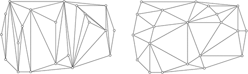
In open areas (meaning areas away from any linear feature) the cartographer generates a Triangulated Irregular Network (TIN) and evaluates the selected soundings against the source information within the triangles and along the edges. There are many ways for generating a TIN from a set of points (e.g. the plane-sweep and Delaunay triangulations illustrated in Figure 1), however it makes more sense for the cartographer (and the mariner, who mentally performs the triangulation in order to interpolate depths in the area) to form triangles from nearby rather than distant soundings, thus to refrain from creating, what is known as, “skinny” triangles. After all, and paraphrasing Tobler’s first law of geography (Tobler 1970) near soundings are more related than distant soundings and that must be considered in the reconstruction of a surface from a bathymetric dataset using a TIN.

Figure 1. Plane-sweep (left) and Delaunay (right) triangulations for the same point dataset (Edelsbrunner 2008).

A triangulation that reduces the skinny triangles is that described by Delaunay (1934). Another advantage of the Delaunay triangulation is that the topology of the triangulation is unique for a given set of generating points, with the exception of degeneracy which occurs in the presence of four or more co-circular points (see Edelsbrunner 2001). This ensures consistency in the TIN construction from the charted bathymetric information, whether this is done by the cartographer during chart compilation, or the mariner when interpolating depths for the safe-navigation of the vessel.

Near linear features, the cartographer evaluates the area of dominance of the selected sounding and the linear feature in question to identify source soundings that deviate from the expected depth. The computational geometry structure that best describes the above thought processes is the Voronoi diagram (Voronoi 1907). From an implementation perspective, the Voronoi regions near depth curves may be incrementally examined with the triangles generated using the Delaunay triangulation.

Both computational data structures (i.e. Delaunay triangulation and Voronoi tessellation) have been used in many areas of geosciences such as geology, meteorology, remote sensing and cartography (Okabe, Boots, and Sugihara 1992), and for a variety of applications, e.g. representation and maintenance of topology in maps (Gold, Rammele, and Roos 1997), terrain modelling (Thibault and Gold 2000), cluster analysis (Ahuja 1982), spatial interpolation (Watson 1992), maritime boundaries delimitation (Kastrisios and Tsoulos 2016), nearest service areas (Kastrisios and Tsoulos 2018), and cartographic generalization (Peters, Ledoux, and Meijers 2014).

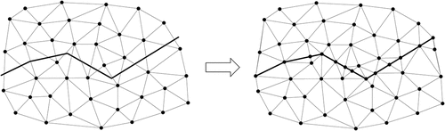
For the presented algorithms and their implementation in this paper, we generate the conforming Delaunay triangulation for all point and linear features carrying bathymetric information (e.g. soundings, rocks, depth curves, coastlines) which have been selected for inclusion in the chart. The advantage of the conforming over the ordinary Delaunay triangulation is that it ensures that the resulting Delaunay edges will not cross the linear features (Figure 2), something that would, otherwise, yield many false positives and make the validation near linear features problematic.

Figure 2. Ordinary Delaunay triangulation (left) and the conforming Delaunay triangulation for a set of points and a linear feature (right).

3. Algorithm

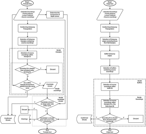
This Section presents the proposed algorithms for the implementation of the triangle (Section 3.1) and the edge (Section 3.2) tests that are also outlined in the flowcharts of Figure 3. The proposed algorithms have been implemented in the Python programming language and the results of a case study are presented in the Results section.

Figure 3. Flowcharts presenting the algorithms for the triangle (left) and edge (right) tests.

3.1. Triangle test

The proposed algorithm for the triangle test is as follows (see the flowchart in Figure 3) :

• (1) Import the features that will be used for the validation, i.e.:

• (a) The selected soundings to be validated.

• (b) All other point and linear features that carry bathymetric information used for the representation of the bottom configuration and the adjacent coastal areas on chart, such as depth curves and coastlines (hereinafter: curves).

• (c) The source soundings.

• (2) Determine the succession of depth curves in the area for later use (e.g. 0 m, 2 m, 5 m, 10 m, 20 m, and 30 m).

• (3) Construct the conforming Delaunay triangulation for the input features of steps (1a) and (1b).

• (4) Select the Delaunay triangles that contain source soundings (the purpose of this step is to reduce the number of spatial queries in the following steps).

• (5) Iterate through the selected Delaunay triangles and for each triangle D_i do the following:

• (a) Select the source soundings within D_i.

• (b) Compare the depth of each of the selected source soundings to the least depth value d_min of the three generators (i.e. the three Delaunay vertices) of the D_i. If the source sounding s_i is deeper than d_min, discard;, otherwise examine the bathymetric features of origin for the three Delaunay vertices forming the D_i:

• (i) If all three vertices are not from the same linear feature (i.e. they do not comprise part of the same curve), the s_i is stored in a dataset containing the confirmed shoals (also: “flags”) as it is shoaler than what the mariner would expect by mentally interpolating the charted depth information in the area.

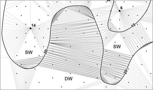
• (ii) If all three vertices do have the same linear feature of origin (i.e. they comprise part of the same curve), the triangle D_i is “flat” and s_i is stored as a candidate shoal (also: “candidate flag”) for further investigation. It is noted that a triangle is “flat” when all three vertices forming the triangle have the same depth value (thus, the triangle has zero slope) but within the context of this work the term is used specifically for the triangles generated by vertices extracted from the same curve. As shown in Figure 4, flat triangles can be generated on both sides of a curve (e.g. the 20m curve in Figure 4). Soundings within flat triangles (shown in grey in Figure 4) on the shallow-water side of the curve (“SW” in Figure 3) are expected to be shoaler than the curve, whereas soundings on its deep-water side (“DW” in Figure 3) must only be deeper.

• (6) Once all triangles have been tested, the algorithm investigates the candidate flags from step 5b(ii) for their position relative to the curves that generated the flat triangles:

• (a) From the candidate flags in the list, those on the deep-waters side of the curve are flagged (based on those discussed in the previous step).

• (b) From the candidate flags that lie on the shallow-water side of the linear feature, those shoaler than the depth value of the next shoaler depth curve in the chart (based on the succession of depth curves determined in step 2) indicate a discontinuity of the succession of depth curves in the area and, as such, must be brought to the attention of the cartographer for the digitization of the respective depth curve (hereinafter: “warnings”). The remaining soundings on the shallow-water side of the polyline, as previously pointed out, are expected to be shoaler than the curve’s assigned depth value and are, therefore, discarded.

Figure 4. Source soundings within flat triangles (shaded areas) on the shallow (SW) and deep-water (DW) side of the 20 m curve require further investigation in terms of their location relatively to the curve before characterizing them as shoals.

The exported results of the above iterative process consist of the “confirmed shoals” (i.e. the source soundings that are shoaler than the least depth of the three depth features forming the triangle) and the “warnings” (i.e. source soundings that imply a discontinuity of depth curves in the area).

3.2. Edge test

The proposed algorithm for the edge-test is as follows (see the flowchart in Figure 3):

• (1) Import the selected point and linear features for inclusion in chart and the source soundings that will be used for the validation (see step 3.1.(1) above).

• (2) Construct the conforming Delaunay triangulation for the above features.

• (3) Remove the Delaunay edges that are part of flat triangles (for those edges the triangle and edge tests would yield the same results and, since the triangle test has already been performed, they may be disregarded for the edge test).

• (4) Create buffers around the remaining edges. The size of the buffer (d) is analogous to the length of the edges using a user-defined value:

(1) $d=k\ast L$(1)

where L the length of the edge, k a user-defined value in the range 0–1, and d the calculated buffer size for the specific edge. The advantage of this approach, instead of using a fixed buffer size for all edges, is that the size of the search area along the edge is analogous to the length of the edge and the density of the charted bathymetric information.

• (5) Select the buffers (polygons) that contain source soundings (the purpose of this step is to reduce the number of spatial queries in the following steps).

• (6) Iterate through the subset of buffers and for each buffer B_i of the Delaunay edge E_i, do the following:

• (a) Select the source soundings within the selected buffer B_i.

• (b) From the selection of source soundings keep only those within the corresponding triangles D_i1 and D_i2. The purpose of this step is to avoid the evaluation of source soundings outside the area of interest.

• (c) Compare the depth of each of the selected source soundings s_i to the least depth value d_min of the two source soundings forming the Delaunay edge E_i (i.e. the Delaunay vertices). If the source sounding s_i is shoaler than d_min, it is flagged.

• (7) Export results, i.e. the source soundings that are shoaler than the least depth of the two depth features forming the edge (“shoals”).

4. Results

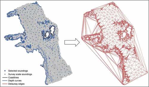
For the evaluation of the proposed algorithms and the implementation of the two tests, a case study is presented with data provided by NOAA/OCS covering an area of 58 km². The dataset comprises 407 selected soundings for validation, 175 closed and floating depth curves and coastlines, and 28,516 source soundings (it is noted that modifications have been made to these so that various cases can be examined). Once the data is loaded, the algorithm constructs the conforming Delaunay triangulation for the point and linear features, according to step 3 of paragraph 3.1 (Figure 5).

Figure 5. The input point and linear features and the resulting conforming Delaunay triangulation.

For this specific dataset, the succession of curves, following step 2 in paragraph 3.1, is 0 m, 5.4 m, 9.1 m, 18.2 m, 91.4 m, and 182.8 m, the metric equivalents with decimeter precision of the charted curves in U.S. standard units, i.e. 0, 18, 30, 60, 300, and 600 ft.

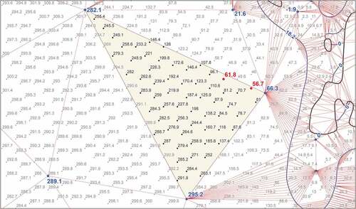
Subsequently, the algorithm performs the validation of the selected soundings following steps 3 through 6 as described in paragraph 3.1 for the triangle test. Figure 6 presents an example of the validation of soundings within a triangle following the iterative process described in step 5 of the same paragraph. Soundings 56.7 m and 61.8 m (shown in red in Figure 6) are flagged as they are shoaler than the least value of the three selected soundings forming the triangle under investigation (i.e. the soundings 66.3 m, 282.1 m, and 295.2 m shown in blue in the same Figure).

Figure 6. Within each triangle, the triangle test identifies the source soundings that are shoaler than the three vertices defining the triangle and flags them.

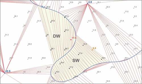
Figure 7 presents an example of flat triangles on both sides of a depth curve (18.2 m) and that, following the procedure described in steps 5b(ii) and 6 of paragraph 3.1, the algorithm identified sounding 17.5 m (shown in red in Figure 7) as a shoal and sounding 8.6 m (shown in orange color in the same Figure) as a warning sounding indicating the absence of a 9.1 m depth curve surrounding it (that is, the next shoaler depth curve).

Figure 7. A confirmed shoal (17.5 m) on the deep-water side of a curve and a “warning” (8.6 m) on the shallow-water side of the depth curve that indicates the absence of a curve with VALDCO 9.1 m surrounding it.

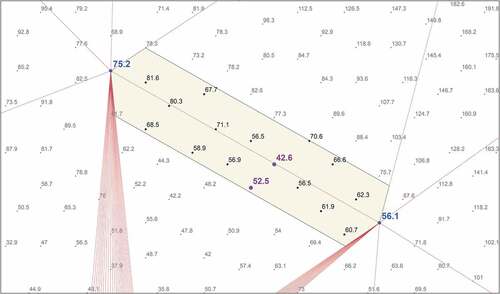
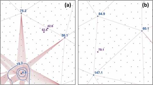
Once the triangle test is complete, the edge test is performed utilizing the conforming Delaunay triangles constructed for the triangle test following the procedure described in paragraph 3.2. For the buffer, a value of k = 0.1 was used in equation (1). Figure 8 presents a specific example of a Delaunay edge formed by two selected soundings with depth values 56.1 m and 75.2 m. The algorithm identified and flagged two source soundings within the buffer (42.6 m and 52.5 m in purple in Figure 8) that violate the mandates of IHO publications for the edge test.

Figure 8. The edge test identifies the two soundings 42.6 m and 52.5 m that are shoaler than the selected soundings 56.1 m, 75.2 m forming an edge and flags them.

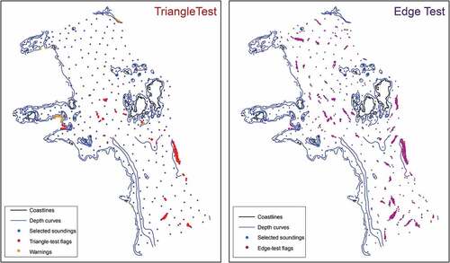
Figure 9 illustrates the exported results of the automated algorithms for the triangle and edge tests for the specific case study. The triangle test identified 128 shoals and 28 warnings, whereas the edge test identified 707 shoals.

Figure 9. The flags and warnings resulted from the triangle test (left) and the flags from the edge test (right) for a factor k = 0.1.

The advantage of incorporating the entirety of the bathymetric information is the improved performance of the tests near and within linear features. Figure 10 provides an illustration of the results of the proposed algorithm for the triangle test (hereinafter: “proposed implementation”), to an implementation that constructed the TIN using only the selected soundings and without taking into account the linear features in the area (following a verbatim interpretation as written in S-4 that “no actual sounding exists within a triangle of selected soundings”) (hereinafter: “other implementation”). It is obvious that in open areas and away from linear features both implementations perform satisfactorily as they successfully identify the shoal soundings (e.g. the two flags marked with “A” in the south-western side of Figure 10). However, near linear features the other implementation (Figure 10(a)) performs poorly as it returns an enormous number of false positives (e.g. area “B” in Figure 10(a)), contrary to the proposed implementation (Figure 10b) which flagged only the actual shoals in these areas (“C” in Figure 10(b)).

Figure 10. (a) The triangle test using only the selected soundings for the construction of the TIN, and (b) the proposed implementation which incorporates all the available bathymetric information from the selected soundings, depth curves, and coastlines.

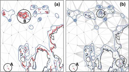
Figure 10 illustrates the improved performance of the proposed implementation over the other implementation for a specific region of the study area near and within linear features. The following comparison of the exported results for the entire area emphasizes the superiority of the proposed methodology and implementation. The proposed implementation flagged 128 source soundings and returned an additional 28 as warnings. The other implementation flagged 1285 source soundings with only 46 being actual shoals and the remaining 96.4% of the flagged soundings being false positives. A fully quantitative comparison is difficult due to the enormous number of false positives from the other implementation that undermines its reliability, especially near linear features. In addition, the warnings found with the proposed implementation are new to this work and, thus, not available with the other implementation.

Figure 11 illustrates the importance of the edge test in the validation process showing two geographic areas with three shoals that the triangle test failed to identify. More precisely, in Figure 11(a) the soundings 42.6 m and 52.5 m were flagged with the edge test as they are shoaler than the two selected soundings forming the edge (i.e. soundings 56.1 m and 75.2 m). In terms of the triangle test, the soundings in question are deeper than the adjacent 18.2 m depth curve, a vertex of which forms the local triangle, and, as such, are not shoals. Likewise, in Figure 11(b) the edge test flagged the sounding 79.1 m which deviates significantly from the expected depth in the area but was not detected by the triangle test due to the third selected sounding (60.1 m) forming the local triangle which is shoaler than the flagged sounding. The presented shoals, identified by the edge test, violate the safety constraint and, therefore, the trio of soundings in these areas must be properly amended.

Figure 11. The significance of the edge test in identifying shoals that the triangle test, by definition, may not detect.

5. Limitations of the two tests

This Section presents the limitations of the triangle and edge tests as part of a fully automated solution for the validation of selected soundings. Figure 11, highlighted the significance of the edge test in the validation process as it may identify shoals that the triangle test fails to identify. Relying solely on the triangle test is therefore inadvisable.

The performance of the edge test depends on the selected buffer size. With a small buffer size, the test fails to identify shoals that lie further from the edge but which are still shoaler than the expected depth, whereas a big buffer size results in examining and, most likely, flagging soundings distant from the edge that are expected to be shoaler than the two soundings forming the edge under investigation. Based on tests performed in the context of this work, a buffer size of about 10% the edge’s length [i.e. k = 0.1 in equation (1)] generally works well but the optimal value remains an open research topic.

A common limitation shared by the two tests concerns the boundaries of the areas under investigation. Due to the absence of the bathymetric information from the adjoining charts, the distribution of charted soundings is violated and, as a consequence, elongated edges are generated (see Figure 5) which prevent the proper evaluation of the corresponding charted soundings. That specific limitation is an implementation deficiency which is expected to be resolved by incorporating the charted soundings from the adjoining charts of the same compilation scale.

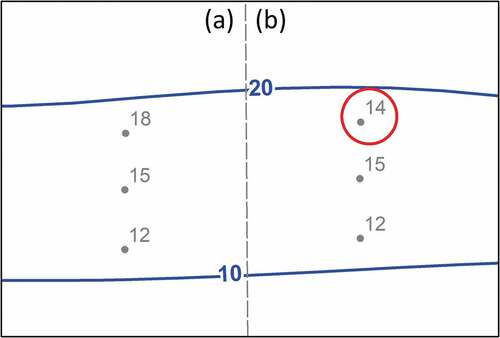
Figures 12–14 demonstrate the fundamental limitation of the two tests as components of a fully automated validation solution. Figure 12 illustrates two depth curves (10 m and 20 m) and the source soundings between the two. On the left side of the dividing line (Figure 12(a)), the values of the three source soundings follow the distribution that one would expect between the portrayed depth curves. On the other side of the dividing line (Figure 12(b)), however, the 14 m sounding near the 20 m depth curve is significantly shoaler than what we would expect at this location, and, as such, must be brought to the cartographer’s attention for further evaluation. However, the specific shoal may not be found with the two tests as it is deeper than the shoalest depth value of the vertices forming the triangles and edges surrounding it (i.e. the comparison depth is 10 m for all vertices from depth curves 10 m and 20 m). Clearly, the described limitation is independent of any algorithmic implementation and can be considered as “intrinsic” to the two tests.

Figure 12. Source sounding (14 m) that deviates significantly from the expected depth but both tests, by definition, may not identify.

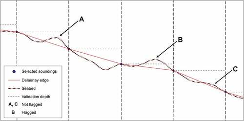
In practice, the two tests generate a rough approximation of the surface represented by the charted bathymetric information using a gridding approach with an enormously big element, either hexagonal (when the edge test is performed) or triangular (when the triangle test is performed) in shape. Each element is assigned the depth value of the shoalest of the two or three vertices forming the edge or triangle, respectively, and is compared to all source soundings within the specific element for the validation process. The deficiency of this approach is that it fails to reconstruct the interpolated surface at the appropriate resolution for the validation tests and to identify local, small-scale variations of the seabed and, thus, discrepancies. To illustrate this, Figure 13 presents a profile view of the seabed based on the available source information (brown-dotted line in Figure 13) and the Delaunay faces (red lines in Figure 13) generated from the selected soundings (blue points in Figure 13). The horizontal-dashed lines represent the vertical section of the elements which are used for identifying areas where the safety constraint is violated. As shown, with this approach only the eminences crossing the horizontal-dashed lines are flagged (e.g. shoal “B” in Figure 13), whereas anything below the validation depth are not (“A” and “C” in Figure 13), even if they deviate significantly from what would be expected by interpolating the charted bathymetric information in the area (shoal “A” in Figure 12) (it is noted that the specific case of eminence “A” simulates the vertical profile of the case described with the support of Figure 12).

Figure 13. A profile view of the seabed, the selected soundings, and the Delaunay faces showing why the two tests fail to identify eminences that deviate significantly from the expected depth on chart.

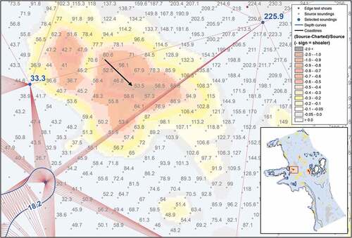
Figure 14 presents a real-world example of the fundamental “intrinsic” limitation of the two tests. For the presented area, which is located on the western part of the dataset used in the Results section (see inset in Figure 14), the source soundings satisfy both the triangle and edge tests, albeit the charted information fails to maintain and emphasize the morphological details and characteristic features of the seafloor and, thus, it violates the safety constraint. The underlying raster represents the difference between the actual source surface and the surface derived from the charted information. Characteristically, at the location of the 53.5 m source sounding (see arrow in Figure 14), the expected depth based on the charted bathymetric information is 109 m (using linear interpolation), thus it appears more than 100% deeper (legend value −1.0) than the actual depth.

Figure 14. Area where the source soundings satisfy both tests but the interpolated surface appears twice deep as the actual source surface, a clear violation of the safety constraint.

6. Discussion and future work

• Normally, at the stage of the validation of selected soundings the depth areas have already been encoded. Thus, the procedure described in paragraph 3.1 for the investigation of whether a candidate flag lies within the shallow or deep-water side of the curve is solved with spatial point-in-polygon queries between the candidate flags and the two depth areas associated with the depth curve. However, if the depth areas do not exist (e.g. depth areas do not comprise part of the deliverables of the Office of Coast Survey HCell [NOAA 2016]) Voronoi tessellation may be used (Kastrisios and Calder 2018).

• Notwithstanding that the Voronoi and point-in-polygon approaches tackle the problem of soundings’ validation within flat triangles, future work will consider the potential computational gain with the skeleton-crust approach (Thibault and Gold 2000) for the elimination of flat triangles and the surface reconstruction from the charted bathymetric information.

• In the Limitations section, we presented the limitations of the triangle and edge tests in a fully automated solution. For one of them (associated with the third shoalest vertex of the triangle test) the issue is solved by applying the edge test. For buffer size and elongated edges, it constitutes part of our future work to determine the best buffer size and shape and to incorporate the charted bathymetric information from the adjoining charts using a buffer around the study area. It is expected that these will improve the performance of the automated implementations of the two tests.

• However, the intrinsic limitation of the two tests presented with the support of Figures 12–14 show that a fully automated validation process based solely on the two tests in their current form does not seem feasible. Discrepancies that the experienced eye of the cartographer may find, cannot be found with utilizing the two tests. A new test that will complement or supersede the two tests for the automated validation of charted soundings is therefore required. It seems logical that the new test will be a surface based test, which will calculate the difference between the source surface and the surface interpolated from the charted information and will identify discrepancies between the two at the appropriate scale. The model that will be used for the surface reconstruction from the charted information is an open question, but by way of example, in (Masetti, Faulkes, and Kastrisios 2018), the simplest extension model (of comparison to 2.5D triangles rather than the shoalest vertex on the 2D triangles as here) is demonstrated in the related field of detecting discrepancies between new survey data and existing charts. In practice, this helps to minimize discrepancies, reducing the number of false positives declared, but at the scale of the chart is still a significant approximation. More nuanced, human-centric, reconstruction methods are probably indicated for the general solution.

• Lastly, the tolerance between the expected and the source depth that should be reported as shoal is not clear (e.g. for a source sounding of 200 m, should or should not an expected depth of, e.g. 199 m be flagged?). It seems logical that tolerance values will vary for the different depth areas (i.e. smaller tolerance for shallow water, larger tolerance for deeper water) and that there must be a link to the Category Zone of Confidence (CATZOC) (IHO 2002) (in its current or a future form) that are used to highlight the accuracy of data presented on charts.

7. Conclusion

This paper presented an algorithmic implementation of the triangle and edge tests for the validation of charted soundings. For the triangulation, we utilized the conforming Delaunay triangulation for the point and linear features carrying bathymetric information on charts. In a case study with data from NOAA/OCS, this paper presented the improved performance of the triangle test near depth curves and coastlines, as well as the importance of the edge test proving that it should not be disregarded by cartographers in the validation process. It also presented limitations associated with the current implementations, which we believe may be solved in the context of future work, and the intrinsic limitation of the triangle and edge tests that prevent the development of a fully automated solution solely relying on them. Lastly, it discussed the need for a new, most likely surface based, test that will complement or supersede the existing two tests and which will comprise part of the future work towards full automation in nautical cartography.

Additional information

Funding

This work is supported by the National Oceanic and Atmospheric Administration [grant number NA15NOS4000200].

Notes on contributors

Christos Kastrisios

Christos Kastrisios is a research scientist with the Center for Coastal and Ocean Mapping/University of New Hampshire. He received his PhD in Cartography from the National Technical University of Athens, Greece for his work on the scientific aspects of maritime delimitation. His research interests are maritime delimitation, cartographic generalization, and computational cartography.

Brian Calder

Brian Calder is a Research Associate Professor and the Associate Director of the Center for Coastal and Ocean Mapping/University of New Hampshire. He has a PhD in Electrical and Electronic Engineering, completing his thesis on Bayesian methods in Sidescan Sonar processing in 1997. His research interests include methods for error modeling, propagation and visualization, and adaptive sonar backscatter modeling.

Giuseppe Masetti

Giuseppe Masetti is a research Assistant Professor with the Center for Coastal and Ocean Mapping/University of New Hampshire. He received his PhD degree in System Monitoring and Environmental Risk Management from the University of Genoa, Italy. His research interest include methods to improve survey data acquisition and processing, with a focus on acoustic seafloor characterization.

Peter Holmberg

Peter Holmberg received a B.S. degree in Geography from Oregon State University in 2001. He joined NOAA in 2001 as in intern and was hired as a Physical Scientist in 2002. He is the Cartographic Team Leader at Pacific Hydrographic Branch where he oversees compilation of hydrographic data to chart scale deliverables which are applied to NOAA’s suite of nautical charts.

References

- Ahuja, N. 1982. “Dot Pattern Processing Using Voronoi Neighborhoods.” IEEE Transactions on Pattern Analysis and Machine Intelligence 4 (3): 336–343. doi:10.1109/TPAMI.1982.4767255.
- Alexander, L. 2003. “Electronic Charts.” In The American Practical Navigator. 199–215 Bethesda, MD: National Imaging and Mapping Agency.
- Delaunay, B. 1934. “Sur la sphère vide. A la mémoire de Georges Voronoï.” Bulletin de l'Académie des Sciences de l'URSS. Classe des sciences mathématiques et na 6: 793–800.
- Du, J., Y. Lu, and J. Zhai. 2001. “A Model of Sounding Generalization Based on Recognition of Terrain Features.” Paper presented at the Proceedings of the 20th International Cartographic Conference, Beijing, China, August 6–10.
- Edelsbrunner, H. 2001. Geometry and Topology for Mesh Generation. Cambridge: Cambridge University Press.
- Edelsbrunner, H. 2008. “Delaunay Triangulations, Design and Analysis of Algorithms CPS230, Duke University,” Accessed 21 November 2008, https://www2.cs.duke.edu/courses/fall08/cps230/
- Gold, C. M., P. R. Rammele, and T. Roos. 1997. “Voronoi Methods in GIS.” In Algorithmic Foundations of Geographic Information Systems, edited by M. van Rreveld, J. Nievergelt, T. Roos, and P. Widmayer, 21–35. Berlin: Springer.
- Hecht, H., A. Kampfer, and L. Alexander. 2007. “The WEND Concept for Worldwide ENC - past or Future: A Review of Progress and A Look to the Future.” International Hydrographic Review 8: 73–79.
- IHO (International Hydrographic Organization). 1994. Hydrographic Dictionary. Publication S-32. 5th ed. Monaco: International Hydrographic Bureau.
- IHO (International Hydrographic Organization). 2000. IHO Transfer Standard for Digital Hydrographic Data. Publication S-57. 3.1 ed. Monaco: International Hydrographic Bureau.
- IHO (International Hydrographic Organization). 2002. IHO Transfer Standard for Digital Hydrographic Data. Publication S-57. S-57 Maintenance Document, Number 8. Monaco: International Hydrographic Bureau.
- IHO (International Hydrographic Organization). 2017. Regulations of the IHO for International (INT) Charts and Chart Specifications of the IHO. Publication S-4. 4.7.0 ed. Monaco: International Hydrographic Organization.
- IMO (International Maritime Organization). 1974. “International Convention for the Safety of Life At Sea (SOLAS), 1 November 1974, 1184 UNTS 3”, Accessed 16 September 2018. http://www.refworld.org/docid/46920bf32.html
- IMO (International Maritime Organization). 2000. Adoption of Amendments to the International Convention for the Safety of Life at Sea (SOLAS), 1974. Revision to Chapter V – Safety of Navigation. IMO Resolution MSC.99(73). adopted on December 5. London: International Maritime Organization.
- IMO (International Maritime Organization). 2006. Adoption of the Revised Performance Standards for Electronic Chart Display and Information Systems (ECDIS). IMO Resolution MSC.232(82). adopted on 5 December 2006. London: International Maritime Organization.
- IMO (International Maritime Organization). 2009. Adoption of Amendments to the International Convention for the Safety of Life at Sea (SOLAS). IMO Resolution MSC.282(86). 5 June 2009. London: International Maritime Organization.
- Kastrisios, C., and B. Calder. 2018. “Algorithmic Implementation of the Triangle Test for the Validation of Charted Soundings.” Paper presented at the Proceedings of the 7th International Conference on Cartography and GIS, Sozopol, Bulgaria, June 18–23. doi: 10.13140/RG.2.2.12745.39528.
- Kastrisios, C., and M. Pilikou. 2017. “Nautical Cartography Competences and Their Effect to the Realisation of a Worldwide Electronic Navigational Charts Database, the Performance of ECDIS and the Fulfilment of IMO Chart Carriage Requirements.” Marine Policy 75: 29–37.doi: 10.1016/j.marpol.2016.10.007.
- Kastrisios, C., and L. Tsoulos. 2016. “A Cohesive Methodology for the Delimitation of Maritime Zones and Boundaries.” Ocean & Coastal Management 130: 188–195. doi:10.1016/j.ocecoaman.2016.06.015.
- Kastrisios, C., and L. Tsoulos. 2018. “Voronoi Tessellation on the Ellipsoidal Earth for Vector Data.” International Journal of Geographical Information Science 32 (8): 1541–1557. doi:10.1080/13658816.2018.1434890.
- MacDonald, G. 1984. “Computer Assisted Sounding Selection Techniques.” The International Hydrographic Review 61 (1): 93–109.
- Masetti, G., T. Faulkes, and C. Kastrisios. 2018. “Automated Identification of Discrepancies between Nautical Charts and Survey Soundings.” ISPRS International Journal of Geo-Information 7 (10): 392.
- NOAA (National Oceanic and Atmospheric Administration). 2016. “U.S. Department of Commerce, Office of Coast Survey.” In Office of Coast Survey HCell Specifications, 29. Silver Spring, MD: National Oceanic and Atmospheric Administration.
- NOAA (National Oceanic and Atmospheric Administration). 2017. “Office of Coast Survey, Marine Chart Division.” In National Charting Plan. A Strategy to Transform Nautical Charting. https://nauticalcharts.noaa.gov/publications/docs/national-charting-plan.pdf
- NOAA (National Oceanic and Atmospheric Administration). 2018. “U.S. Department of Commerce, Office of Coast Survey.” In Nautical Chart Manual. Volume 1 - Policies and Procedures. Version 2018.2, 897. Silver Spring, MD: National Oceanic and Atmospheric Administration.
- Okabe, A., B. Boots, and K. Sugihara. 1992. Spatial Tessellations - Concepts and Applications of Voronoi Diagrams. Chichester: John Wiley and Sons.
- Oraas, S. R. 1975. “Automated Sounding Selection.” The International Hydrographic Review 52 (2): 103–115.
- Peters, R., H. Ledoux, and M. Meijers. 2014. “A Voronoi-Based Approach to Generating Depth-Contours for Hydrographic Charts.” Marine Geodesy 37 (2): 145–166. doi:10.1080/01490419.2014.902882.
- SCALGO (Scalable Algorithmics). 2017. SCALGO Nautical Documentation, 59. Release 1.17.0. Aarhus, Denmark: Scalable Algorithmics. https://scalgo.com/en-US
- Sui, H., P. Cheng, A. Zhang, and J. Gong. 1999. “An Algorithm for Automatic Cartographic Sounding Selection.” Geo-Spatial Information Science 2 (1): 96–99. doi:10.1007/BF02826726.
- Sui, H., X. Zhu, and A. Zhang. 2005. “A System for Fast Cartographic Sounding Selection.” Marine Geodesy 28 (2): 159–165. doi:10.1080/01490410590953695.
- Thibault, D., and C. M. Gold. 2000. “Terrain Reconstruction from Contours by Skeleton Construction.” GeoInformatica 4 (4): 349–373. doi:10.1023/A:1026509828354.
- Tobler, W. R. 1970. “A Computer Movie Simulating Urban Growth in the Detroit Region.” Economic Geography 46 (sup1): 234–240. doi:10.2307/143141.
- Tsoulos, L., ., and K. Stefanakis. 1997. “Sounding Selection for Nautical Charts: An Expert System Approach.” Paper presented at the Proceedings of the 18th International Cartographic Conference, Stockholm, Sweden, June 23–27.
- Voronoi, G. 1907. “Nouvelles Applications Des Paramètres Continus À La Théorie Des Formes Quadratiques. Premier Mémoire: Sur Quelques Propriétées Des Formes Quadritiques Positives Parfaites.” Math 133: 97–178.
- Watson, D. F. 1992. Contouring: A Guide to the Analysis and Display of Spatial Data. Oxford: Pergamon.
- Wilson, M., G. Masetti, and B. Calder. 2016. “NOAA QC Tools: Origin, Development, and Future.” Paper presented at the 2016 Canadian Hydrographic Conference, Halifax, Nova Scotia, Canada, May 16–19.
- Yu, W. 2018. “Automatic Sounding Generalization in Nautical Chart considering Bathymetry Complexity Variations.” Marine Geodesy 41 (1): 68–85.
- Zhang, X., and E. Guilbert. 2011. “A Multi-Agent System Approach for Feature-Driven Generalization of Isobathymetric Line.” In Advances in Cartography and GIScience. Volume 1. Lecture Notes in Geoinformation and Cartography, edited by A. Ruas, 477–495. Berlin: Springer. doi:10.1007/978-3-642-19143-5_27.
- Zoraster, S., and S. Bayer. 1992. “Automated Cartographic Sounding Selection.” International Hydrographic Review 59 (1): 57–61.