Integrating VGI and 2D hydraulic models into a data assimilation framework for real time flood forecasting and mapping

ABSTRACT

Crowdsourced data can effectively observe environmental and urban ecosystem processes. The use of data produced by untrained people into flood forecasting models may effectively allow Early Warning Systems (EWS) to better perform while support decision-making to reduce the fatalities and economic losses due to inundation hazard. In this work, we develop a Data Assimilation (DA) method integrating Volunteered Geographic Information (VGI) and a 2D hydraulic model and we test its performances. The proposed framework seeks to extend the capabilities and performances of standard DA works, based on the use of traditional in situ sensors, by assimilating VGI while managing and taking into account the uncertainties related to the quality, and the location and timing of the entire set of observational data. The November 2012 flood in the Italian Tiber River basin was selected as the case study. Results show improvements of the model in terms of uncertainty with a significant persistence of the model updating after the integration of the VGI, even in the case of use of few-selected observations gathered from social media. This will encourage further research in the use of VGI for EWS considering the exponential increase of quality and quantity of smartphone and social media user worldwide.

KEYWORDS:

• Crowdsourced data
• VGI
• data assimilation (DA)
• flood forecasting
• 2D hydraulic modelling

1. Introduction

Hydrologic and hydraulic modeling for rainfall-runoff and river flow routing simulations are currently implemented within Early Warning Systems (EWS) for managing and mitigating the devastating impact of floods in urban ecosystems (e.g. Krzhizhanovskaya et al. 2011; Alfieri, Pappenberger, and Wetterhall 2014; Girons Lopez, Di Baldassarre, and Seibert 2017). EWS generally incorporate Data assimilation (DA) algorithms for managing the uncertainty of physically based river channel flow simulations towards more accurate and timely efficient forecasting of flood wave propagation along fluvial valleys. DA supports hydrodynamic modeling for making optimal use of the different and diverse water stage observation systems. Assimilation of river flow observations (McLaughlin 2002; Moradkhani et al. 2005; Liu and Gupta 2007) and remotely sensed data (Matgen et al. 2010; García-Pintado et al. 2013) constitute the two main components of DA-based EWS. However, while in-channel levee-protected river high flows are easier to forecast using 1D hydraulic models, especially in gauged systems, several challenges affect DA when dealing with over-bank distributed floodplain flow propagation. This issue is mainly affecting ungauged basins but also gauged rivers considering the lack or uncertainty, when available, of distributed out-of-channel water level sensors and remotely sensed information. In this regard, remote sensing technology is progressing at an unprecedented pace with radar and optical images that are available with Earth Observation (EO) data and platforms that capture flood dynamics from the global to the local scale. Nevertheless, flood modeling is still a pivotal asset of EWS considering that EO data are not timely available for the satellite orbit revisit time and vegetation cover that impact optical images. As a result, research on novel DA frameworks that integrate out-of-channel flood flow observations, making optimal use of all the diverse potential water observation information is, thus, crucial for more effective and accurate numerical simulations supporting EWS in understanding and forecasting hazardous events.

Among the innovative source of inundation observations, data gathered by citizens, or crowdsourced data, are characterized by great potential, but also a significant challenge. Georeferenced information produced by citizens is now largely and freely available thanks to the spreading of smartphones and social media users, even in developing countries (Hilbert 2016). Spatial information is voluntarily collected by citizens and published online using social networks (e.g. Facebook, Instagram, etc.). Additionally, the increasing number of custom-made platforms and web applications is demonstrating the need and importance of user-driven flood observations (e.g. Horita et al. 2015). This novel source of data seems to be very promising for supporting flood forecasting from global to local scales, but significant efforts are still needed before using such data in practice. Several projects tested the use of water observations taken by citizens for water resource and risk management (e.g. Buytaert et al. 2014; Van Meerveld, Vis, and Seibert 2017), but the use of crowdsourced data for real-time flood forecasting have not been fully explored yet.

Flickr and Twitter seem the most used social media for getting crowdsourced information related to disasters, allowing all public data to be found and extracted using their Application Programming Interfaces (API). Images captured from video streams by Youtube are also used. In this context, the analysis and interpretation of the media content for organizing, collecting, positioning and extracting relevant information is an active research topic with specific regard to the extraction of geotagged information from social media streams (e.g. Schindler et al. 2008; Luo et al. 2011).

Different definitions and acronyms are usually used to refer to water, territorial and environmental monitoring data gathered and disseminated by citizens. Volunteered Geographic Information (VGI, Goodchild 2007) refers to the general principle of citizens volunteering for collecting georeferenced information and is commonly used within the geospatial and GIS communities. Other definitions and acronyms are also adopted without strictly considering the spatial reference, such as Crowdsourced Data (CD), User Generated Content (UGC). For a more comprehensive list see Table 1. In this manuscript, we select and use the acronym VGI.

Table 1. List of definitions for data gathered from citizens (adapted from Assumpção et al. 2018).

Name	Source
Citizen science	Irwin 1995
Citizen observatory	Degrossi et al. 2014
Citizen sensing	Foody et al. 2013
Trained volunteers	Gallart et al. 2016
Participatory data collection methods	Michelsen et al. 2016
Crowdsourcing	Leibovici et al. 2017
Participatory sensing	Kotovirta et al. 2014
Community-based monitoring	Conrad and Hilchey 2011
Volunteered geographic information	Goodchild 2007
Eyewitnesses	Poser and Dransch 2010
Non-authoritative sources	Schnebele et al. 2014
Human sensor network	Aulov, Price, and Halem 2014
Crowdsourced geographic information	See et al. 2016

Several research works present recent findings concerning the use of VGI for water resource and risk management (e.g. Bonney et al. 2014). Buytaert et al. (2014) give some examples of citizen engagement in hydrology and water science specifying also the type of data that are continuously collected by citizens and that may serve this purpose.

Outcomes of these projects and researches are encouraging in demonstrating the possibility of effectively observing climatic and hydrologic processes (Muller et al. 2015). Social media data have been used for directly creating deterministic or probabilistic flood maps from citizen-observed water levels (McDougall 2011; McDougall and Temple-Watts 2012; Fohringer et al. 2015), stream discharges (Le Boursicaud et al. 2016; Le Coz et al. 2016), flood extent (Schnebele et al. 2014; Cervone et al. 2016; Le Coz et al. 2016; Li et al. 2018; Rosser, Leibovici, and Jackson 2017), or just their geotagged position (Eilander et al. 2016; Brouwer et al. 2017; Poser and Dransch 2010; Triglav-Čekada and Radovan 2013; Schnebele and Waters 2014; Sun et al. 2016; Holderness and Turpin 2015).

Crowdsourced data have been also integrated for validating flood models. Aulov, Price, and Halem (2014) developed a platform (AsonMaps) for a rough estimation of water levels and flood/non-flood areas early validation of the surge model forecasts. Fava et al. (2014) integrated the voluntary prediction models with short-term information, to fill the gaps of the traditional observed data for improving the flood forecasting. Kutija et al. (2014) gathered information from a web page for validating and calibrating a hydrodynamic model. Smith et al. (2015) validated GPU accelerated hydrodynamic modeling with crowdsourced information for real-time flood forecasting in an urban environment. Yu, Yin, and Liu (2016) validated a 2D urban hydro-inundation model integrating traditional observation with reported localized flood incidents at the street or house level by the public. Mazzoleni et al. (2015), Mazzoleni et al. (2018) demonstrated the benefits of assimilating both traditional and VGI observations with simplified hydrological and hydraulic modeling for improving the flood prediction. Nevertheless, further research is needed to test the assimilation of crowdsourced data in real scenarios adopting more advanced models and considering other uncertainties related to VGI, such as the ones on the location and the timing.

The principal issue affecting the use of VGI for flood analysis is the uncertainty and low reliability resulting from the use of such data. While VGI are still considered as qualitative information, there is a significant potential of using VGI as quantitative water observation information, but the uncertainty of the information has to be carefully evaluated. The uncertainty analysis is expressed as a function of the citizen technological equipment, the experience, the credibility (e.g. random citizens versus trained volunteer) and any further information characterizing the citizen-driven VGI gathering process that impact the accuracy, completeness and precision of the water observation (Tulloch and Szabo 2012; Bordogna et al. 2014). Reliability assessments require ad hoc statistical tools to evaluate the random error and bias to be assigned to the observation (e.g. Bird et al. 2014). Data reliability can be assessed considering not only the expertise and methodology that characterizes the data source but also the time and the position in which that information is sensed and processed. To address this issue, semantic rules governing what can occur at a given location can be used as a filter for observations (Vandecasteele and Devillers 2013) or taking the mean and the standard deviation of compared measurements at predefined time windows (Mazzoleni et al. 2018).

While an exponentially increasing number of investigations are working towards a quantitative use of crowdsourced information (Assumpção et al. 2018), we could not find many researches attempting to integrate VGI into DA frameworks for improving EWS performances. Additionally, the few case studies implementing VGI for DA-based flood forecasting adopt simplified hydrologic and hydraulic models, and 1D hydraulic algorithms in particular (Mazzoleni et al. 2015, 2018). Exploiting the full potential of citizen-driven flood hazard and risk management and modeling systems, also integrating VGI, require a comprehensive simulation of the floodplain spatially distributed water dynamics that 1D hydraulic models cannot provide. VGI and 2D hydraulic models shall be, thus, jointly considered and implemented for DA of EWS frameworks that effectively consider all the diverse data sources as well as the physical and human processes hat interplay towards more accurate and efficient flood early warning and inundation hazard management.

This research tries to address this important missing component of VGI use for flood modeling studies by developing a research that: (a) implement and test a DA framework using VGI and a 2D hydraulic model; (b) use VGI effectively for flood risk management; and (c) use a real case study to evaluate advantages and limitations of the proposed approach.

The paper is organized as follows: In Section 2 the case study of the Tiber River is presented, with specific subsections on input data and available VGI for the selected flood event. In Section 3 the models and methods are described, with specific regard to the forecasting hydrologic and hydraulic models and the DA methodology, focusing on the modeling and the observational error analysis. Results are, then, presented in Section 4 and conclusions are given in Section 5.

2. Case study

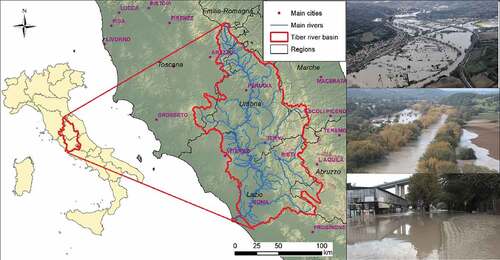
The selected case study is the Tiber River basin, the second largest catchment in Italy. In particular, the fluvial segment from Orte Scalo to the Castel Giubileo dam is selected, located just upstream of the city center of Rome in central Italy (bounding box of the domain ranges between 42.6° and 43.85°N and 11.8°–12.9° E in the Lazio region, Figure 1). The catchment area at the Orte Scalo node has an extension of 5881 km², with several minor tributaries contributing downstream to the main river (such as Treja, Farfa, Corese, Aja Di Poggio tributaries), and only one main tributary represented by the Nera river (4180 km²) that lead to an overall extension of the basin at the Castel Giubileo downstream node of 15,086 km². Elevations for the entire basin range from a maximum of 2470 m above sea level (a.s.l.) to a minimum of – 6 m a.s.l. with an average elevation of 524 m (a.s.l.). Land use is predominantly associated with cultivated lands (~55%) with also forests (~40%) and urbanized areas (~5%). The climatic and hydrologic regime of the Tiber River basin is characterized by variable and intense precipitation with most of the total annual rainfall (average yearly cumulated precipitation of 1020 mm/year, Romano and Preziosi 2013) occurring in autumn and spring, following a Mediterranean regime. The Tiber River is often subject of flooding conditions, which impact the selected river segment and also the historical city center of Rome (Tauro et al. 2016; Nardi, Annis, and Biscarini 2018a). The hydrologic regime of the upstream boundary condition is governed by the Corbara dam, located 40 km from the Orte Scalo node, and the Paglia River confluence, just downstream of the Corbara dam, that control the flooding routing dynamics of the Orte Scalo – Castel Giubileo fluvial valley. This river reach is strategically important for the flood risk management of the Rome city center, considering the flood wave expansion and attenuation within the Orte-Castel Giubileo floodplain.

Figure 1. The Tiber River basin case study: river basin boundary and network with identification of the main boundary conditions of the domain of interest. The right insets include images from recent flood events in the Orte-Castel Giubileo floodplain.

2.1. Available material and data

The increasing frequency of inundation events in the Tiber River basin (Brunetti et al. 2004; Fiseha et al. 2014) motivated the development of a flood hazard modeling and mapping updating program (also known as PS1), that was commissioned in 2012 by Lazio Region and Tiber River Basin Authority. The hydrologic and hydraulic modeling study consisted in the gathering, processing and modeling of updated topographic and bathymetric data (Table 2) for the creation of a robust and accurate geospatial dataset representing the geometry of the fluvial bottom. Additionally available datasets consist in the river discharge/stage rating tables and observation of recent flood events that were gathered from the Lazio Region Civil Protection agency for the main bridges and weirs. Land use data (Corine Land Cover at the fourth level for the whole national territory provided by Istituto Superiore per la Protezione e la Ricerca Ambientale, ISPRA) were also gathered for the hydrologic parametrization of floodplain landscape within the domain of study. Hydraulic parameters (e.g. roughness parameters) were calibrated using observation from recent floods to build a consistent flood wave routing model that was implemented to simulate the ground effect of synthetic design hydrographs for predefined recurrence intervals (50, 200 and 500 years return time). The different maximum potential flooding extents were consequently identified upon the hydrologic forcing scenarios for urban planning and regional zoning purposes. The hydrology and the implemented hydraulic model, represented by a 2D hydraulic algorithm, are gathered and used as reference material and methods for this research.

Table 2. Topographic data sources and layers.

Data type	Name	Data format	Data content	Resolution specs.	Notes/source
Vector	Surveyed cross sections	Shapefile	N/A	N/A	Sparse and inconsistent covering in space and time/Tiber River basin authority
Raster	Lidar DTM	ASCII grid	Digital Terrain model of the fluvial buffer for the entire domain	1 m	Minister of environment PST dataset
Raster	Regione Lazio DTM	ASCII grid	Digital Terrain model of the entire basin	5 m	Regione Lazio

2.2. Crowdsourced data

The 2012 flood event was selected as a reference test case. VGI from structured volunteering projects (e.g. phone apps, custom web apps) are not available for the study domain. Nevertheless, social network users are generally very active considering the high density of population that characterizes the Tiber fluvial valley in the proximity of the city of Rome. Unconventional data sources, Youtube, in particular, were used. Twitter Search API was also queried, but valuable information for a DA implementation was not found. From the several available video streams, a small subset of videos of the flooding was found of particular interest in the visual observation of water levels in recognizable locations. The detailed georeferencing of the images was possible using the tags of the posts and also by matching the crowdsourced picture with google street view. The geocoding of the captured media location was, thus, finalized and a small number (less than 20) of flood observation nodes were identified within the computational domain in correspondence of three urbanized areas (Orte Scalo, Torrita Tiberina and Monterotondo) that were severely affected by the Tiber River flooding (Figure 2). Additional-crowdsourced images were gathered from the internet, news articles and social network (Twitter in particular), providing additional-crowdsourced material, even if the selected flood event took place six years earlier than this work. The presented web crawling activity, with youtube video extraction combined with internet search using as keywords the date, the place and common hashtags (e.g. #Tiber, #flood), supported the identification of a total of three water observations (Table 3) to be considered suitable for being used as potentially quantitative observation for the proposed procedure.

Table 3. Selected VGI images.

No.	Location	Source	Date – Time
1	Orte Scalo	Youtube	14/11/2012–10:00 am
2	Torrita Tiberina	Youtube	14/11/2012–09:00 am
3	Monteronondo	Youtube	14/11/2012–13:30 am

Figure 2. Location of the crowdsourced images selected for the November 2012 Tiber River flood event.

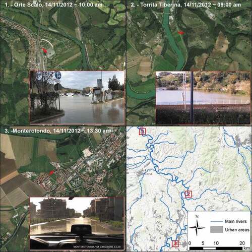
The selected VGI are characterized by uncertainties in their spatial and temporal localization. The positions of the VGI images were verified by visual comparison with Google Maps Street View images. For these locations, high-resolution digital terrain elevation of the LiDAR data was available for evaluating the elevation in dry condition. A visual analysis of the water depths by the comparison of wet (VGI images) versus dry (Google Maps Street View images) conditions of the affected areas was performed.

The methodology can be replicated in near real time for the same purpose adopting the Application Programming Interface (API) of the social media platform that allow to filter geotagged information selecting keywords related to the flood event. This process can be automatized using semantic filtering and deep learning. Tkachenko, Jarvis, and Procter (2017) demonstrated the potential of using polysemous tags of images in the Flickr database as support of early warning of an event before its outbreak. Brouwer et al. (2017) used the Twitter streaming API for spatially and semantically filter tweets related to the analyzed flood event. Jiang et al. (2018) adopted transfer learning and lasso regression for waterlogging depth extraction from video images. An advanced algorithm for extracting information from the twitter platform for disaster response was recently developed, such as TAGGS (de Bruijn et al. 2018).

3. Models and methods

3.1. Flood modeling

The selected inundation model is based on the combination of a hydrological rainfall-runoff model and of a 2D river flow routing algorithm.

The hydrologic model is based on the Instantaneous Unit Hydrograph (IUH) rainfall-runoff model implementing the width function (WF); the WF characterizes the shape of the runoff response to the unit precipitation pulse by analyzing the travel time distribution of surface runoff at the basin scale (Grimaldi, Petroselli, and Nardi 2012). In particular, the WFIUH implements DEM-based terrain analysis, interpolation and processing for simulating the runoff response to the precipitation input using a IUH that is expressed as a function of the geomorphic structure of the river network and predefined surface flow dynamics (i.e. channel and hillslope surface flow velocities assigned as a function of catchment feature morphologic and land use properties) (Rodríguez-Iturbe and Valdes 1979; Grimaldi, Teles, and Bras 2004, Grimaldi, Teles, and Bras 2005; Petroselli and Grimaldi 2018). This hydrologic model, that was calibrated using real events, is able to transform rainfall observations, gathered from the Tiber basin monitoring network, into a runoff for estimating the hydrograph to be used as upstream boundary conditions for the hydraulic routing model.

The selected 2D river flow routing algorithm is the FLO-2D PRO software. It is a physically based process model able to simulate the flood wave routing over unconfined flow surfaces (2D equations) using the dynamic wave approximation to the momentum equation (O’Brien, Julien, and Fullerton 1993). FLO-2D routes the flood hydrograph on the gridded floodplain surface simulating the channel flow propagation and the channel-floodplain overbank exchange, and the interaction of floodplain flow dynamics with urban features and obstructions (e.g. levees, culverts, bridges, embankments, buildings). FLO-2D is a volume conservation model, using the Manning coefficient to represent terrain roughness, solving the De Saint Venant equations. FLO-2D is defined as a Quasi-2D model considering that the channel is represented using cross sections and a 1D geometry linked to the unconfined gridded surface where the flow, overflowing from the 1D channel, is propagated using a fully dynamic 2D wave routing.

For the presented case study, a grid resolution equal to 150 m was set, interpolating topographic data from high resolution 1-meter LiDAR dataset. This resolution proved to be a good compromise between computational effort and accuracy of results (Peña and Nardi 2018). In situ surveyed cross sections were adopted for representing the geometry of the river channel. Boundary conditions were assigned considering both the flow measurements in the upstream part of the Tiber River and the flow hydrographs from 15 ungauged basins simulated by the adopted WFIUH hydrologic model. The computational domain was optimized adopting a hydrogeomorphic model (Nardi, Vivoni, and Grimaldi 2006; Nardi et al. 2018b; Morrison et al. 2018) according to Annis et al. (2019) approach.

The distribution of the Manning values for the floodplain surface within the study domain was evaluated using reference values extracted from literature (varying between 0.02 and 0.20 m^–1/3s) associating roughness conditions to land use classes of the Corine Land Cover project at the fourth level provided by the Italian Institute for Environmental Protection and Research (ISPRA) for the whole Italian country. Manning values of the channel were calibrated and validated considering three flood events (2012 flood event for calibration; 2005 and 2010 flood events for validation) and four stage gauges stations (Ponte Felice, Stimigliano, Nazzano, Ponte del Grillo) comparing the observed water depths with the simulated ones. Reasonable values of Nash-Sutcliffe-Efficiency coefficients (NSE varying between 0.4 and 0.9), Pearson correlations (0.85–0.98) and Bias (0.98–1.10), were obtained confirming the validity of the calibration procedure. However, lower values of NSE (0.2–0.4) for the 2005 and 2010 event were obtained for Nazzano and Ponte del Grillo stations.

3.2. DA model

In this work, the Ensemble Kalman Filter (EnKF) method (Evensen 2003) is applied to the selected Quasi-2D hydraulic model. The EnKF model is a sequential DA method that estimates the unknown model state (e.g. flood flow depth) based on the available observations at each time step. Specifically, the updated probability density function (pdf) of the model state is given by a combination between the data likelihood and the forecasted pdf of the model states by means of a Bayesian update. The forecast (a priori) state error covariance matrix is approximated propagating the ensemble of the model states, considering its uncertainties, from the previous time step. At the same time, an ensemble of observations at each update time is generated according to their error distribution introducing a noise term. If a set of observations $y_{t+1}$ is taken at time $t+1$, these can be assimilated into the model. The observation for the i-th ensemble member can be expressed as:

(1) $\begin{array}{c}{\hat{y}}_{t+1}^i=y_{t+1}+{\eta }_{t+1}^i,{\eta }_{t+1}^i\sim N\left(0,R_{t+1}^y\right)\end{array}$(1)

where $y_{t+1}=H\left(x_{t+1},\theta \right)$ is the observation at time t +1, $H\left(\dots \right)$ is a propagator that links the state variables to the measured variables providing the expected value of the output given the model state and parameters. ${\eta }_{t+1}^i$ is the noise, considering a random normal distribution with zero mean and variance $R_{t+1}^y$, usually considered time dependent.

The state variable $x_{t+1}^{i-}$ of forecast model in the EnKF, for the i-element of the ensemble at a time $t+1$ can be expressed as:

(2) $\begin{array}{ccc}{x}_{t+1}^{i-}=M\left(x_t^{i+},I_t^i,{\theta }_i,t\right)+w_t^i& \hspace{0.17em}& i=1,\dots ,n\end{array}$(2)

where $x_t^{i+}$ is the i^th updated ensemble member at time $t$, $w_t^i$ is the model error of the i^th ensemble member, generated randomly. The forcing input $I_t^i$ and the parameters ${\theta }_i$ of the i^th ensemble member are generated starting from the deterministic value and adding a random normal error with zero mean and a certain variance, namely $I_t^i=I_t+N\left(0,S_t^I\right)$ and ${\theta }_i=\theta +N\left(0,S^{\theta }\right)$. From the a priori estimate of the state variable ${\bar{x}}_{t+1}^{-}$, the posterior estimate ${\bar{x}}_{t+1}^{+}$ is calculated using the observation $y_{t+1}$ performing a linear correction with the Kalman filter to the forecasted state ensemble members:

(3) $x_{t+1}^{i+}=x_{t+1}^{i-}+K_{t+1}\left(y_{t+1}^i-{\hat{y}}_{t+1}^i\right)$(3)

where $K_{t+1}$ is the Kalman gain matrix, expressed as:

(4) $K_{t+1}=\frac{P_{t+1}^{-}{H}^{\mathrm{T}}}{H{P}_{t+1}^{-}{H}^{\mathrm{T}}+R_{t+1}^y}$(4)

where $P_{t+1}^{-}$ is the ensemble covariance matrix; $H$ is the observation transition operation and $R_{t+1}^y$ is the variance of the observation error.

In this work, the state variable $x_t^{\hspace{0.17em}}$ is the water depth in a specific location of the computational domain. In case of crowdsourced information, like a photo depicting water depths or a quantitative description of flood depths from any web content, the state variable can be located both in the channel or more likely in the floodplain. The non-linear function (…) introduced in Equation (2) is the hydraulic model engine, whose forcing term I_t is the ensemble of the flow hydrographs, and the parameters θ are the channel and floodplain roughness. The model error w_t is estimated considering the uncertainties related by the input forcing and the model parameters. The observation y_t is a water depth value gathered from the VGI. For this reason, the observation transition operation H is an identity matrix, being a direct relation between state variable and observation. The perturbation v_t to be assigned to the observation ensemble is strongly dependent on the nature of the observation, as described in Section 3.4. The correction of the model states in the 2D hydraulic domain is enforced into the floodplain cell where the observation is located, but also to both the closest channel cell and to the floodplain cells that are hydraulically connected to the channel cell. A propagation of the correction upstream and downstream is, thus, performed adopting a gain function similar to Madsen and Skotner (2005) since the correction of only one channel cell would bring instability to the flood wave routing model. This correction propagation model is also weighted by implementing a spatially varying correction factor that varies as a function of the distance of the corrected location. Specifically, the correction propagation function weights are proportional to the inverse of the distance between the analyzed channel cell and the channel cell connected to the floodplain cell where the observation is located. In the following subsections, the procedure for taking into account the model errors (Section 3.3) and the observation errors (Section 3.4) in order generate the ensembles of the forecast state variables and the observations to be implemented in the EnKF framework are illustrated. Section 3.4 presents one of the main novelty of the proposed work, concerning the approached tested for managing the uncertainties of VGI into the DA flood EWS approach.

3.3. Errors of the flood forecast model

The EnKF takes in to account the uncertainty related to the model errors through a realization of the model results and in particular by perturbing:

the forcing input given by the static sensors and the hydrologic model;

the model parameters that is the channel roughness expressed by the Manning values.

Following Weerts and El Serafy (2006), the i-element of the hydrologic input at time t is generally expressed with as follows:

(5) ${Q^s}_{t,i}={Q^S}_t+N{\left(0,R_t\right)}^{\hspace{0.17em}}$(5)

where ${Q^S}_t$ is the flow value given by the observation or by the hydrologic model, $N{\left(0,R_t\right)}^{\hspace{0.17em}}$ is a noise term normally distributed with zero mean and the variance $R_t$ that depends on the type of hydrologic input and can be expressed as:

(6) $R_t={\left({\alpha }_t\cdot {Q^{true}}_t\right)}^2$(6)

where ${\alpha }_t$ is the coefficient of variation related to the uncertainty of the input discharge.

The uncertainty related to discharge observation (${\alpha }_{StS,t}$) is given by the sum of two different components (Clark et al. 2008): the estimation of the water level from the static sensor (EWL) and the transformation of the water level into discharge with the rating curve (ERC). In this case study, ${\alpha }_{StS,t}$ has been imposed equal to 0.12, considering the flow rating curve component equal to 0.1 (Weerts and El Serafy 2006) and the component due to the water level estimation equal to 0.02 (Mazzoleni et al. 2015).

The uncertainties affecting the hydrologic model, like the value of the coefficient of variation ${\alpha }_I$, are related to different factors, such as the measured rain and its distribution at the basin scale, the simplified modelling of the flow routing, the neglected physical process (e.g. groundwater flow), the mud and debris flow, the antecedent soil moisture conditions among others. After a calibration analysis of the abovementioned hydrologic model for four small-gauged basins during the 2012 flood event, here not reported for sake of brevity, the coefficient of variation ${\alpha }_I$ is assumed to equal to 0.3. The uncertainty related to the model parameters is considered as follows (Clark et al. 2008; McMillan et al. 2013):

(7) ${p^s}_i=p^s+U\left(-{\epsilon }_P\cdot p^s,+{\epsilon }_P\cdot p^s\right)$(7)

where ${p^s}_i$ is the perturbed model parameter for the i-element of the ensemble, $p^s$ is the model parameter and ${\epsilon }_P$ is the fractional parameter error. In this case, the channel roughness has been chosen as the perturbed parameter and ${\epsilon }_P$ is assumed equal to 0.25. This constrains the value Manning of the channel between 0.30 and 0.50 m^–1/3s.

3.4. Observation errors in crowdsourced data

The observation errors related to VGI are characterized by three different factors: location error, timing error and the water depth estimation error.

3.4.1. Location error ($er{r}_{loc}^{VGI}$)

DA models normally consider the location of observation ascertain. This is reasonable for typical oceanographic or hydrologic measurement methods, so the issue related to a potential location error is still not much investigated in the literature. Locational information of VGI, for example, tweets, can be uncertain because geotags are available for only a very small number of tweets and may significantly differ from the actual location of the observation (Hahmann, Purves, and Burghardt 2014).

If the VGI is a picture, even if the geotagged position is in a wrong place, the image could provide landmarks to place the correct position of the observation, whose location error can be lower than the resolution of the large-scale hydraulic model, thus negligible. If the VGI is a text message from a social platform or it is an image without any recognizable landmark, the geotagged position of the VGI can vary considerably depending on its type (McClanahan and Gokhale 2015; Brouwer et al. 2017). The perturbation of the VGI observation given by the positioning error for the i-element of the ensemble can be expressed as a noise error normally distributed with zero mean and variance $R_{loc}^{VGI}$:

(8) $er{r}_{loc,i}^{VGI}=N\left(0,R_{loc}^{VGI}\right)$(8)

In the adopted hydraulic model, this error can be implemented moving the position of the cells to which a VGI observation is assigned considering the number of times the location error of the i-element of the ensemble is greater than the resolution of the model both for x and y coordinates (Figure 3):

(9) $\left(X_i^{VGI},Y_i^{VGI}\right)=\left(X^{VGI}+N\left(0,R_{loc}^{VGI}\right),Y^{VGI}+N\left(0,R_{loc}^{VGI}\right)\right)$(9)

Figure 3. Example of perturbation error due to location for VGI observation.

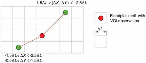
where $X^{VGI}$ and $Y^{VGI}$ are the North and East coordinates of the geotagged VGI.

The variance $R_{loc}^{VGI}$ varies depending on the type of geotagging. Considering a similar approach suggested by Sengupta et al. (2012), for the time step in which an observation is assimilated, if the location of the observation related to i-element of the ensemble $\left(X_i^{VGI},Y_i^{VGI}\right)$ is different to $\left(X^{VGI},Y^{VGI}\right)$, the observation at this location is derived considering how it could be if an observation at $\left(X_i^{VGI},Y_i^{VGI}\right)$ is assimilated. Hence, the water depth at a location $\left(X^{VGI},Y^{VGI}\right)$ is given by:

(10) $W{D}_{\left(X^{VGI},Y^{VGI}\right),t+1}^{+}=W{D}_{\left(X_i^{VGI},Y_i^{VGI}\right),t+1}^{+}+\left(W{D}_{\left(X^{VGI},Y^{VGI}\right),t+1}^{-}-W{D}_{\left(X_i^{VGI},Y_i^{VGI}\right),t+1}^{-}\right)$(10)

In other words, the observation at the original location $\left(X^{VGI},Y^{VGI}\right)$ is measured starting from the observation at the perturbed location $\left(X_i^{VGI},Y_i^{VGI}\right)$ and considering the reciprocal water level differences before the updating step of the DA. The selected VGI data, being images in which landmarks are clearly visible, are affected by a low location error whose variance is imposed equal to $R_{loc}^{VGI}$= 100.

3.4.2. Timing error ($er{r}_{time}^{VGI}$)

The timing error, that is the error of assigning a specific time to a VGI information, is characterized by two components: (a) The error related to the wrong time set in the device: this error is not more than few seconds or few minutes and can be negligible. (b) The lag time between the information acquisition and the user posting time. For (b), if the VGI data has not text reporting the exact time of the information to be used or this information is imprecise, the time between the information acquisition and its sharing by the user can be considerably high, i.e. several hours. In order to take into account this error, the proposed approach tests an error-induced timing of the VGI.

The time step related to the VGI observation of the i-element of the ensemble can be perturbed using the following expression:

(11) $t_i^{VGI}=t_{\hspace{0.17em}}^{VGI}+N\left(0,R_{time}^{VGI}\right)$(11)

where $N\left(0,R_{time}^{VGI}\right)$ is a noise error normally distributed with zero mean and variance $R_{time}^{VGI}$[hours].

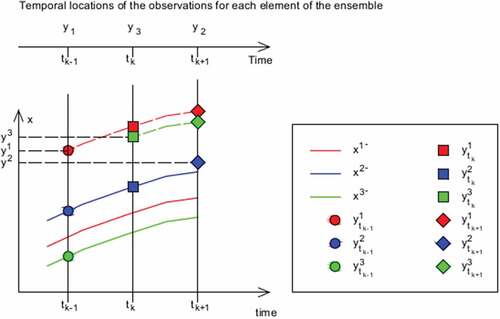
If at time step $t_k$ the i-element of the ensemble is affected by a VGI observation, its correspondent perturbed observation is directly given by Equation (7). If the i-element of the ensemble is not affected by an observation at time $t_k$ but it has been already affected by the observation at time $t_{k-1}$, its water depth observation at time $t_k$ should be the value assumed in case of a correction given by Equation (7) at time $t_{k-1}$. Lastly, if the i-element of the ensemble is not affected by an observation at time $t_k$ but it will be affected by the observation at time $t_{k+1}$, its water depth observation at time $t_k$ should be the value assumed by its variable if no updating has been performed to that simulation at time $t_k$ (Figure 4). In this work, the variance $R_{time}^{VGI}$ associated with the time location related to the VGI images has been imposed equal to 30 min for each image.

Figure 4. Scheme of the perturbation of the ensemble considering the timing error. The continuous lines are the forecasting variables; the dashed lines are the auxiliary simulations to set each time step the value of the observation for every ensemble.

3.4.3. Water depth derivation ($er{r}_{wd}^{VGI}$)

Water surface elevation has been derived by adding the water depth observed from VGI data to the local ground elevation (Fohringer et al. 2015; Brouwer et al. 2017). Water depths can be derived both from image interpretation or from text messages describing the flood dynamics. Brouwer et al. (2017) observed that water depths mentioned by tweet messages are generally higher than the water depths derived from the visual interpretation of the photographs, with errors lower than 55 cm. However, a statistical test could not confirm the mean error in water depth was any different from zero, so the water depth estimation errors have been simulated using a normal distribution with zero mean and a standard deviation of 20 cm.

The water surface elevation has been derived as a sum of the terrain elevation given by the LiDAR DTM and the depth deduced by the visual interpretation of the image. The perturbation of the water surface elevation for the i-element of the ensemble is assigned as follows:

(12) $er{r}_{wse,i}=N\left(0,R_{DEM}\right)+N\left(0,R_{Depth}\right)$(12)

where $R_{DEM}$ is the variance related to the DEM error, assigned equal to 0.3 m and $R_{Depth}$ is the variance of the water depth derivation from visual interpretation, assigned equal to 0.2 m, as in Brouwer et al. (2017). However, a lower limit of 0.05 m has been assigned for the water depth derivation in order not to have negative or zero values of water depths. The water depth has been deduced comparing the images during the flood with the same images get in dry conditions from Google Street View.

4. Results

Here we present a comparative analysis of the inundation modeling using the proposed approach making use of the error correction procedure (updated model) as respect the model run without the correction procedure (non-updated model). Figure 5(b) shows the spatial distribution of the differences between the mean water depths of the updated as compared to the no updated simulations. The vertical correction along the water profile is also represented in Figure 5(d), while the temporal variation is shown in Figure 5(c). The persistence of the correction is about 8 h. Further results of the performance analysis are reported in Table 4.

Table 4. Comparison of the means of the observed, simulated and updated water levels at the location of the VGI observations.

Location	Date – Time	Mean water levels (m)
		Observed	Simulated	Updated
Orte Scalo	14/11/2012–10:00am	10.43	9.44	9.56
Torrita Tiberina	14/11/2012–09:00am	11.74	10.26	10.35
Monterotondo	14/11/2012–13:30am	17.11	16.45	16.72

Figure 5. (a) Location of the VGI image in Torrita Tiberina. (b) Map of the water level correction at the time of the Torrita Tiberina VGI acquisition (09:00 14/11/2012). (c) Hydrograph of the mean water depths at the Torrita Tiberina channel cell. (d) Mean water surface elevation profile considering the updated and no updated simulations.

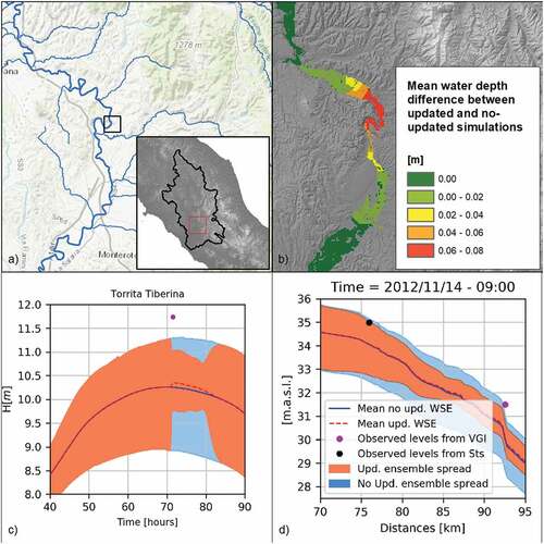
These outcomes suggest that a more significant effect of VGI data for improving the model performance can be obtained with the largest number of observation data, spatially but also temporally distributed at least every few hours, considering that the effect of each observation persists for several hours after its assimilation in the framework.

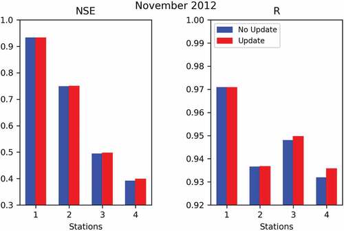
The correction of the water levels does not considerably affect the flood extension considering the mean values of the water surface elevation. For example, at 9:00 am on 14/11/2012, namely at the time of the correction of the VGI data from Torrita Tiberina, the increasing of the flooded areas after the correction is only equal to 0.079 km². Figure 5(b) shows the spatial distribution of the mean water level corrections at the time of the Torrita Tiberina VGI acquisition. The performances of the overall simulation, in terms of Nash–Sutcliffe efficiency and Person Correlation, are calculated considering four different stage gage stations (Figure 6). Since the corrections are local and persist for few hours, the performance improvement in case of updated simulation, compared to the no updating, is almost negligible for the first two stations (in the upstream part of the basin). On the other hand, a slight improvement can be appreciated in the downstream part of the basin.

Figure 6. Performance indexes NSE (Nash–Sutcliffe Efficiency) and R (Pearson Correlation) at 4 stage gage stations (1: Ponte Felice; 2: Stimigliano; 3: Nazzano; 4: Ponte del Grillo).

The effect of the correction procedure is minor, an expected result considering the number of injected VGI observations into the DA procedure, but the aim of the tests, concerning the computational efficiency and accuracy increase of the 2D flood routing model, is encouraging. The proposed methodology implementing a DA-based state variables updating process allowed the 2D hydraulic model to be quite stable after each correction. This seems promising towards the adoption of larger spatially distributed datasets of VGI during flood events.

5. Conclusions

In this work, VGI data are used in a DA framework to investigate potential improvements in the performances of 2D hydraulic models for flood forecasting. A new methodology was tested for taking into account all the sources of uncertainties of the citizen information, including the timing and location errors. This work was motivated by the need for investigating new sources of information to cope with data scarcity issues that affect river basin flood risk management and mitigation globally. In fact, while expensive ground monitoring systems (i.e. gauges) seem inaccessible, especially in developing countries, citizen data are rapidly spreading in urban areas worldwide (Statista 2017). Nevertheless, a reliability assessment of VGI observation is a key factor for their successful integration into flood hazard forecasting models.

A case study was developed for testing the proposed approach and the November 2012 flood event in the Tiber River basin was selected for the availability of traditional flood observations, VGI together with a calibrated detailed topographic, hydrologic and hydraulic model. The available flood modeling was integrated into a novel DA framework using the EnKF in order to consider the uncertainty related to the VGI observation. Results show slight, but consistent improvements in the performance of the flood simulations assimilating VGI, an expected result considering the few VGI injected into the model. This encourages the development of additional tests for evaluating the potentially improved performances in case studies with a larger number of VGI data. Integration of spatially distributed VGI in floodplain domains with other sources of information such as stage gages and satellite remotely sensed data can be a challenge for improving the flood forecasting. Moreover, additional analysis of the timing and location errors that characterize these kinds of information using a richer data environment for their validation could give more support on the modeling of their probability distribution.

Additional information

Notes on contributors

Antonio Annis

Antonio Annis is a post-doc researcher at the Water Resources Research and Documentation Centre (WARREDOC) of University for Foreigners of Perugia. He received his PhD joint degree from the University of Florence and the Technical University of Braunschweig. His research interests include integration of remotely sensed data and crowdsourced information in to hydraulic modelling and hydrogeomorphic models for floodplain mapping.

Fernando Nardi

Fernando Nardi is an associate professor of University for Foreigners of Perugia where he also serves as Director of the Water Resources Research and Documentation Centre (WARREDOC). He received his PhD degree in hydrology from Sapienza University of Rome. His research interests pertain to numerical and geospatial modelling for hydrology, hydraulics, geomorphology, Citizen Science and Big Data applications within flood risk and water resource management research projects.

References

- Alfieri, L., F. Pappenberger, and F. Wetterhall. 2014. “The Extreme Runoff Index for Flood Early Warning in Europe.” Natural Hazards and Earth System Sciences 14 (6): 1505–1515. doi:10.5194/nhess-14-1505-2014.
- Annis, A., F. Nardi, R. R. Morrison, and F. Castelli. 2019. “Investigating Hydrogeomorphic Floodplain Mapping Performance with Varying DTM Resolution and Stream Order.” Hydrological Sciences Journal ( (accepted)). doi:10.1080/02626667.2019.1591623.
- Assumpção, T. H., I. Popescu, A. Jonoski, and D. P. Solomatine. 2018. “Citizen Observations Contributing to Flood Modelling: Opportunities and Challenges.” Hydrology and Earth System Sciences 22 (2): 1473–1489. doi:10.5194/hess-22-1473-2018.
- Aulov, O., A. Price, and M. Halem. 2014. “AsonMaps: A Platform for Aggregation Visualization and Analysis of Disaster Related Human Sensor Network Observations.” Paper presented at the 11th International ISCRAM Conference, University Park, PA, May 19–20.
- Bird, T. J., A. E. Bates, J. S. Lefcheck, N. A. Hill, R. J. Thomson, G. J. Edgar, R. D. Stuart-Smith, et al. 2014. “Statistical Solutions for Error and Bias in Global Citizen Science Datasets.” Biological Conservation 173 :144–154. doi:10.1016/j.biocon.2013.07.037.
- Bonney, R., J. L. Shirk, T. B. Phillips, A. Wiggins, H. L. Ballard, A. J. Miller-Rushing, and J. K. Parrish. 2014. “Next Steps for Citizen Science.” Science 343 (6178): 1436–1437. doi:10.1126/science.1251554.
- Bordogna, G., P. Carrara, L. Criscuolo, M. Pepe, and A. Rampini. 2014. “A Linguistic Decision Making Approach to Assess the Quality of Volunteer Geographic Information for Citizen Science.” Information Sciences 258: 312–327. doi:10.1016/j.ins.2013.07.013.
- Brouwer, T., D. Eilander, A. van Loenen, M. J. Booij, K. M. Wijnberg, J. S. Verkade, and J. Wagemaker. 2017. “Probabilistic Flood Extent Estimates from Social Media Flood Observations.” Natural Hazards and Earth System Sciences 17 (5): 735. doi:10.5194/nhess-17-735-2017.
- Brunetti, M., L. Buffoni, F. Mangianti, M. Maugeri, and T. Nanni. 2004. “Temperature, Precipitation and Extreme Events during the Last Century in Italy.” Global and Planetary Change 40 (1–2): 141–149. doi:10.1016/S0921-8181(03)00104-8.
- Buytaert, W., Z. Zulkafli, S. Grainger, L. Acosta, T. C. Alemie, J. Bastiaensen, B. De Bièvre, et al. 2014. “Citizen Science in Hydrology and Water Resources: Opportunities for Knowledge Generation, Ecosystem Service Management, and Sustainable Development.” Frontiers in Earth Science 2 :26. doi:10.3389/feart.2014.00026.
- Cervone, G., E. Sava, Q. Huang, E. Schnebele, J. Harrison, and N. Waters. 2016. “Using Twitter for Tasking Remote-Sensing Data Collection and Damage Assessment: 2013 Boulder Flood Case Study.” International Journal of Remote Sensing 37 (1): 100–124. doi:10.1080/01431161.2015.1117684.
- Clark, M. P., D. E. Rupp, R. A. Woods, X. Zheng, R. P. Ibbitt, A. G. Slater, J. Schmidt, and M. J. Uddstrom. 2008. “Hydrological Data Assimilation with the Ensemble Kalman Filter: Use of Streamflow Observations to Update States in a Distributed Hydrological Model.” Advances in Water Resources 31 (10): 1309–1324. doi:10.1016/j.advwatres.2008.06.005.
- Conrad, C. C., and K. G. Hilchey. 2011. “A Review of Citizen Science and Community-Based Environmental Monitoring: Issues and Opportunities.” Environmental Monitoring and Assessment 176: 273–291. doi:10.1007/s10661-010-1582-5.
- de Bruijn, J. A., H. de Moel, B. Jongman, J. Wagemaker, and J. C. Aerts. 2018. “TAGGS: Grouping Tweets to Improve Global Geoparsing for Disaster Response.” Journal of Geovisualization and Spatial Analysis 2 (1): 2. doi:10.1007/s41651-017-0010-6.
- Degrossi, L. C., J. Porto De Albuquerque, M. C. Fava, and E. M. Mendiondo. 2014. “Flood Citizen Observatory? A Crowdsourcing-Based Approach for Flood Risk Management in Brazil.” Paper presented at the International Conference on Software Engineering and Knowledge Engineering SEKE, Vancouver, July 1–3, pp 570–575.
- Eilander, D., P. Trambauer, J. Wagemaker, and A. van Loenen. 2016. “Harvesting Social Media for Generation of near Real-Time Flood Maps.” Procedia Engineering 154: 176–183. doi:10.1016/j.proeng.2016.07.441.
- Evensen, G. 2003. “The Ensemble Kalman Filter: Theoretical Formulation and Practical Implementation.” Ocean Dynamics 3 (4): 343–367. doi:10.1007/s10236-003-0036-9.
- Fava, C., G. Santana, D. A. Bressiani, A. Rosa, F. E. A. Horita, V. C. B. Souza, and E. M. Mendiondo. 2014. “Integration of Information Technology Systems for Flood Forecasting with Hybrid Data Sources.” Paper presented at the International Conference of Flood Management, Sao Paolo, Brazil, September 16–18.
- Fiseha, B. M., S. G. Setegn, A. M. Melesse, E. Volpi,And, and A. Fiori. 2014. “Impact of Climate Change on the Hydrology of Upper Tiber River Basin Using Bias Corrected Regional Climate Model.” Water Resources Management 28 (5): 1327–1343. doi:10.1007/s11269-014-0546-x.
- Fohringer, J., D. Dransch, H. Kreibich, and K. Schröter. 2015. “Social Media as an Information Source for Rapid Flood Inundation Mapping.” Natural Hazards and Earth System Sciences 15 (12): 2725–2738. doi:10.5194/nhess-15-2725-2015.
- Foody, G. M., L. See, S. Fritz, M. Van der Velde, C. Perger, C. Schill, and D. S. Boyd. 2013. “Assessing the Accuracy of Volunteered Geographic Information Arising from Multiple Contributors to an Internet Based Collaborative Project.” Transactions in GIS 17: 847–860. doi:10.1111/tgis.12033.
- Gallart, F., P. Llorens, J. Latron, N. Cid, M. Rieradevall, and N. Prat. 2016. “Validating Alternative Methodologies to Estimate the Regime of Temporary Rivers When Flow Data are Unavailable.” Science of the Total Environment 565: 1001–1010. doi:10.1016/j.scitotenv.2016.05.116.
- García-Pintado, J., J. C. Neal, D. C. Mason, S. L. Dance, and P. D. Bates. 2013. “Scheduling Satellite-Based SAR Acquisition for Sequential Assimilation of Water Level Observations into Flood Modelling.” Journal of Hydrology 495: 252–266. doi:10.1016/j.jhydrol.2013.03.050.
- Girons Lopez, M., G. Di Baldassarre, and J. Seibert. 2017. “Impact of Social Preparedness on Flood Early Warning Systems.” Water Resources Research 53 (1): 522–534. doi:10.1002/2016WR019387.
- Goodchild, M. F. 2007. “Citizens as Sensors: The World of Volunteered Geography.” GeoJournal 69 (4): 211–221. doi:10.1007/s10708-007-9111-y.
- Grimaldi, S., A. Petroselli, and F. Nardi. 2012. “A Parsimonious Geomorphological Unit Hydrograph for Rainfall–Runoff Modelling in Small Ungauged Basins.” Hydrological Sciences Journal 57 (1): 73–83. doi:10.1080/02626667.2011.636045.
- Grimaldi, S., V. Teles, and R. L. Bras. 2004. “Sensitivity of a Physically Based Method for Terrain Interpolation to Initial Conditions and Its Conditioning on Stream Location.” Earth Surface Processes and Landforms 29 (5): 587–597. doi:10.1002/esp.1053.
- Grimaldi, S., V. Teles, and R. L. Bras. 2005. “Preserving First and Second Moments of the Slope Area Relationship during the Interpolation of Digital Elevation Models.” Advances in Water Resources 28 (6): 583–588. doi:10.1016/j.advwatres.2004.11.014.
- Hahmann, S., R. S. Purves, and D. Burghardt. 2014. “Twitter Location (Sometimes) Matters: Exploring the Relationship between Georeferenced Tweet Content and Nearby Feature Classes.” Journal of Spatial Information Science 9: 1–36. doi:10.5311/JOSIS.2014.9.185.
- Hilbert, M. 2016. “Big Data for Development: A Review of Promises and Challenges.” Development Policy Review 34 (1): 135–174. doi:10.1111/dpr.12142.
- Holderness, T., and E. Turpin. 2015. “From Social Media to GeoSocial Intelligence: Crowdsourcing Civic Co-Management for Flood Response in Jakarta, Indonesia.” In The Social Media for Government Services, edited by S. Nepal, C. Paris, and D. Georgakopoulos, 115–133. Switzerland: Springer International Publishing. doi:10.1007/978-3-319-27237-5_6.
- Horita, F. E., J. P. de Albuquerque, L. C. Degrossi, E. M. Mendiondo, and J. Ueyama. 2015. “Development of a Spatial Decision Support System for Flood Risk Management in Brazil that Combines Volunteered Geographic Information with Wireless Sensor Networks.” Computers & Geosciences 80: 84–94. doi:10.1016/j.cageo.2015.04.001.
- Irwin, A. 1995. Citizen Science: A Study of People, Expertise and Sustainable Development. London: Psychology Press, Routledge. doi:10.4324/9780203202395.
- Jiang, J., J. Liu, C. Z. Qin, and D. Wang. 2018. “Extraction of Urban Waterlogging Depth from Video Images Using Transfer Learning.” Water 10 (10): 1485. doi:10.3390/w10101485.
- Kotovirta, V., T. Toivanen, M. Järvinen, M. Lindholm, and K. Kallio. 2014. “Participatory Surface Algal Bloom Monitoring in Finland in 2011–2013.” Environmental Systems Research 3: 24. doi:10.1186/s40068-014-0024-8.
- Krzhizhanovskaya, V. V., G. S. Shirshov, N. B. Melnikova, R. G. Belleman, F. I. Rusadi, B. J. Broekhuijsen, B. P. Gouldbyd, et al. 2011. “Flood Early Warning System: Design, Implementation and Computational Modules.” Procedia Computer Science 4 :106–115. doi:10.1016/j.procs.2011.04.012.
- Kutija, V., R. Bertsch, V. Glenis, D. Alderson, G. Parkin, C. L. Walsh, J. Robinson, and C. Kilsby. 2014. “Model Validation Using Crowd-Sourced Data From A Large Pluvial Flood.” Paper presented at the 11th International Conference on Hydroinformatics, New York, USA, August 17–21.
- Le Boursicaud, R., L. Pénard, A. Hauet, F. Thollet, and J. Le Coz. 2016. “Gauging Extreme Floods on YouTube: Application of LSPIV to Home Movies for the Post‐Event Determination of Stream Discharges.” Hydrological Processes 30 (1): 90–105. doi:10.1002/hyp.10532.
- Le Coz, J., A. Patalano, D. Collins, N. F. Guillén, C. M. García, G. M. Smart, J. Bind, et al. 2016. “Crowdsourced Data for Flood Hydrology: Feedback from Recent Citizen Science Projects in Argentina, France and New Zealand.” Journal of Hydrology 541 :766–777. doi:10.1016/j.jhydrol.2016.07.036.
- Leibovici, D., J. Rosser, C. Hodges, B. Evans, M. Jackson, and C. Higgins. 2017. “On Data Quality Assurance and Conflation Entanglement in Crowdsourcing for Environmental Studies.” ISPRS International Journal of Geo-Information 6 (3): 1–17, 78. doi:10.3390/ijgi6030078.
- Li, Z., C. Wang, C. T. Emrich, and D. Guo. 2018. “A Novel Approach to Leveraging Social Media for Rapid Flood Mapping: A Case Study of the 2015 South Carolina Floods.” Cartography and Geographic Information Science 45 (2): 97–110. doi:10.1080/15230406.2016.1271356.
- Liu, Y., and H. V. Gupta. 2007. “Uncertainty in Hydrologic Modeling: Toward an Integrated Data Assimilation Framework.” Water Resources Research 43 (7): 1–18. doi:10.1029/2006WR005756.
- Luo, J., D. Joshi, J. Yu, and A. Gallagher. 2011. “Geotagging in Multimedia and Computer Vision – A Survey.” Multimedia Tools and Applications 51 (1): 187–211. doi:10.1007/s11042-010-0623-y.
- Madsen, H., and C. Skotner. 2005. “Adaptive State Updating in Real-Time River Flow Forecasting—A Combined Filtering and Error Forecasting Procedure.” Journal of Hydrology 308 (1–4): 302–312. doi:10.1016/j.jhydrol.2004.10.030.
- Matgen, P., M. Montanari, R. Hostache, L. Pfister, L. Hoffmann, D. Plaza, V. R. N. Pauwels, G. J. M. De Lannoy, R. De Keyser, and H. H. Savenije. 2010. “Towards the Sequential Assimilation of SAR-derived Water Stages into Hydraulic Models Using the Particle Filter: Proof of Concept.” Hydrology and Earth System Sciences 14 (9): 1773–1785. doi:10.5194/hess-14-1773-2010.
- Mazzoleni, M., L. Alfonso, J. Chacon-Hurtado, and D. Solomatine. 2015. “Assimilating Uncertain, Dynamic and Intermittent Streamflow Observations in Hydrological Models.” Advances in Water Resources 83: 323–339. doi:10.1016/j.advwatres.2015.07.004.
- Mazzoleni, M., V. J. Cortes Arevalo, U. Wehn, L. Alfonso, D. Norbiato, M. Monego, M. Ferri, and D. P. Solomatine. 2018. “Exploring the Influence of Citizen Involvement on the Assimilation of Crowdsourced Observations: A Modelling Study Based on the 2013 Flood Event in the Bacchiglione Catchment (Italy).” Hydrology and Earth System Sciences 22 (1): 391–416. doi:10.5194/hess-22-391-2018.
- McClanahan, B., and S. S. Gokhale. 2015. “Location Inference of Social Media Posts at Hyper-Local Scale.” Paper presented at the Future Internet of Things and Cloud (FiCloud), 3rd International Conference on IEEE, Rome, August 24–26, pp. 465–472. doi: 10.1109/FiCloud.2015.71.
- McDougall, K. 2011. “Using Volunteered Information to Map the Queensland Floods.” Paper presented at the Proceedings of the 2011 Surveying and Spatial Sciences Conference: Innovation in Action: Working Smarter (SSSC 2011), Wellington, New Zealand, November 21–25.
- McDougall, K., and P. Temple-Watts. 2012. “The Use of LiDAR and Volunteered Geographic Information to Map Flood Extents and Inundation.” ISPRS Annals of the Photogrammetry, Remote Sensing and Spatial Information Sciences 1: 251–256. doi:10.5194/isprsannals-I-4-251-2012.
- McLaughlin, D. 2002. “An Integrated Approach to Hydrologic Data Assimilation: Interpolation, Smoothing, and Filtering.” Advances in Water Resources 25 (8): 1275–1286. doi:10.1016/S0309-1708(02)00055-6.
- McMillan, H. K., E. Ö. Hreinsson, M. P. Clark, S. K. Singh, C. Zammit, and M. J. Uddstrom. 2013. “Operational Hydrological Data Assimilation with the Recursive Ensemble Kalman Filter.” Hydrology and Earth System Sciences 7 (1): 21. doi:10.5194/hess-17-21-2013.
- Michelsen, N., H. Dirks, S. Schulz, S. Kempe, M. Al-Saud, and C. Schüth. 2016. “YouTube as a Crowd-Generated Water Level Archive.” Science of the Total Environment 568: 189–195. doi:10.1016/j.scitotenv.2016.05.211.
- Moradkhani, H., K. L. Hsu, H. Gupta, and S. Sorooshian. 2005. “Uncertainty Assessment of Hydrologic Model States and Parameters: Sequential Data Assimilation Using the Particle Filter.” Water Resources Research 41 (5): 1–17. doi:10.1029/2004WR003604.
- Morrison, R. R., E. Bray, F. Nardi, A. Annis, and Q. Dong. 2018. “Spatial Relationships of Levees and Wetland Systems within Floodplains of the Wabash Basin, USA.” JAWRA Journal of the American Water Resources Association 54 (4): 934–948. doi:10.1111/1752-1688.12652.
- Muller, C. L., L. Chapman, S. Johnston, C. Kidd, S. Illingworth, G. Foody, A. Overeem, and R. R. Leigh. 2015. “Crowdsourcing for Climate and Atmospheric Sciences: Current Status and Future Potential.” International Journal of Climatology 35 (11): 3185–3203. doi:10.1002/joc.4210.
- Nardi, F., A. Annis, and C. Biscarini. 2018a. “On the Impact of Urbanization on Flood Hydrology of Small Ungauged Basins: The Case Study of the Tiber River Tributary Network within the City of Rome.” Journal of Flood Risk Management 11: S594–S603. doi:10.1111/jfr3.12186.
- Nardi, F., E. R. Vivoni, and S. Grimaldi. 2006. “Investigating a Floodplain Scaling Relation Using a Hydrogeomorphic Delineation Method.” Water Resources Research 42 (9): 1–15. doi:10.1029/2005WR004155.
- Nardi, F., R. R. Morrison, A. Annis, and T. E. Grantham. 2018b. “Hydrologic Scaling for Hydrogeomorphic Floodplain Mapping: Insights into Human-Induced Floodplain Disconnectivity.” River Research and Applications 34 (7): 675–685. doi:10.1002/rra.3296.
- O’Brien, J. S., P. Y. Julien, and W. T. Fullerton. 1993. “Two-Dimensional Water Flood and Mudflow Simulation.” Journal of Hydraulic Engineering 119 (2): 244–261. doi:10.1061/(ASCE)0733-9429(1993)119:2(244).
- Peña, F., and F. Nardi. 2018. “Floodplain Terrain Analysis for Coarse Resolution 2D Flood Modeling.” Hydrology 5 (52): 1–16. doi:10.3390/hydrology5040052.
- Petroselli, A., and S. Grimaldi. 2018. “Design Hydrograph Estimation in Small and Fully Ungauged Basins: A Preliminary Assessment of the EBA4SUB Framework.” Journal of Flood Risk Management 11: S197–S210. doi:10.1111/jfr3.12193.
- Poser, K., and D. Dransch. 2010. “Volunteered Geographic Information for Disaster Management with Application to Rapid Flood Damage Estimation.” Geomatica 64 (1): 89–98.
- Rodríguez‐Iturbe, I., and J. B. Valdes. 1979. “The Geomorphologic Structure of Hydrologic Response.” Water Resources Research 15 (6): 1409–1420. doi:10.1029/WR015i006p01409.
- Romano, E., and E. Preziosi. 2013. “Precipitation Pattern Analysis in the Tiber River Basin (Central Italy) Using Standardized Indices.” International Journal of Climatology 33 (7): 1781–1792. doi:10.1002/joc.3549.
- Rosser, J. F., D. G. Leibovici, and M. J. Jackson. 2017. “Rapid Flood Inundation Mapping Using Social Media, Remote Sensing and Topographic Data.” Natural Hazards 87 (1): 103–120. doi:10.1007/s11069-017-2755-0.
- Schindler, G., P. Krishnamurthy, R. Lublinerman, Y. Liu, and F. Dellaert. 2008. “Detecting and Matching Repeated Patterns for Automatic Geo-Tagging in Urban Environments.” Paper presented at the Computer Vision and Pattern Recognition, 2008, IEEE Conference on, Anchorage, AK, USA, June 23–28, pp. 1–7. doi: 10.1109/CVPR.2008.4587461.
- Schnebele, E., G. Cervone, S. Kumar, and N. Waters. 2014. “Real Time Estimation of the Calgary Floods Using Limited Remote Sensing Data.” Water 6 (2): 381–398. doi:10.3390/w6020381.
- Schnebele, E., and N. Waters. 2014. “Road Assessment after Flood Events Using Non-Authoritative Data.” Natural Hazards and Earth System Science 14 (4): 1007–1015. doi:10.5194/nhess-14-1007-2014.
- See, L., P. Mooney, G. Foody, L. Bastin, A. Comber, J. Estima, S. Fritz, et al. 2016. “Crowdsourcing, Citizen Science or Volunteered Geographic Information? The Current State of Crowdsourced Geographic Information.” ISPRS International Journal of Geo-Information 5 :55. doi:10.3390/ijgi5050055.
- Sengupta, A., S. D. Foster, T. A. Patterson, and M. Bravington. 2012. “Accounting for Location Error in Kalman Filters: Integrating Animal Borne Sensor Data into Assimilation Schemes.” PloS One 7 (8): e42093. doi:10.1371/journal.pone.0042093.
- Smith, L., Q. Liang, P. James, and W. Lin. 2015. “Assessing the Utility of Social Media as a Data Source for Flood Risk Management Using a Real-Time Modelling Framework.” Journal of Flood Risk Management 10 (3): 370–380. doi:10.1111/jfr3.12154.
- Statista. 2017. “Number of Smartphone Users Worldwide from 2014 to 2020 (In Billions).” Source: https://www.statista.com/statistics/330695/number-of-smartphone-users-worldwide/
- Sun, D., S. Li, W. Zheng, A. Croitoru, A. Stefanidis, and M. Goldberg. 2016. “Mapping Floods Due to Hurricane Sandy Using NPP VIIRS and ATMS Data and Geotagged Flickr Imagery.” International Journal of Digital Earth 9 (5): 427–441. doi:10.1080/17538947.2015.1040474.
- Tauro, F., G. Olivieri, A. Petroselli, M. Porfiri, and S. Grimaldi. 2016. “Flow Monitoring with a Camera: A Case Study on a Flood Event in the Tiber River.” Environmental Monitoring and Assessment 188 (2): 118. doi:10.1007/s10661-015-5082-5.
- Tkachenko, N., S. Jarvis, and R. Procter. 2017. “Predicting Floods with Flickr Tags.” PloS One 12 (2): e0172870. doi:10.1371/journal.pone.0172870.
- Triglav-Čekada, M., and D. Radovan. 2013. “Using Volunteered Geographical Information to Map the November 2012 Floods in Slovenia.” Natural Hazards and Earth System Sciences 3 (11): 2753–2762. doi:10.5194/nhess-13-2753-2013.
- Tulloch, A. I., and J. K. Szabo. 2012. “A Behavioural Ecology Approach to Understand Volunteer Surveying for Citizen Science Datasets.” Emu-Austral Ornithology 112 (4): 313–325. doi:10.1071/MU12009.
- Van Meerveld, H. I., M. J. Vis, and J. Seibert. 2017. “Information Content of Stream Level Class Data for Hydrological Model Calibration.” Hydrology and Earth System Sciences 21 (9): 4895. doi:10.5194/hess-21-4895-2017.
- Vandecasteele, A., and R. Devillers. 2013. “Improving Volunteered Geographic Data Quality Using Semantic Similarity Measurements.” ISPRS – International Archives of the Photogrammetry, Remote Sensing and Spatial Information Sciences 1 (1): 143–148. doi:10.5194/isprsarchives-XL-2-W1-143-2013.
- Weerts, A. H., and G. Y. El Serafy. 2006. “Particle Filtering and Ensemble Kalman Filtering for State Updating with Hydrological Conceptual Rainfall–Runoff Models.” Water Resources Research 42 (9): 1–17. doi:10.1029/2005WR004093.
- Yu, D., J. Yin, and M. Liu. 2016. “Validating City-Scale Surface Water Flood Modelling Using Crowd-Sourced Data.” Environmental Research Letters 11 (12): 124011. doi:10.1088/1748-9326/11/12/124011.