Measuring spatio-temporal autocorrelation in time series data of collective human mobility

ABSTRACT

Massive spatio-temporal big data about human mobility have become increasingly available. Revealing underlying dynamic patterns from these data is essential for understanding people’s behavior and urban deployment. Spatio-temporal autocorrelation analysis is an exploratory approach to recognizing data distribution in space and time. The most widely used spatial autocorrelation measurements, such as Moran’s I and local indicators of spatial association (LISA), only apply to static data, so are powerless to spatio-temporal big data about human mobility. Thus, we proposed a new method by extending Moran’s I to measure the spatial autocorrelation of time series data. Then the method was applied to taxi ride data in Beijing, China to reveal the spatial pattern of collective human mobility. The result shows that there is strong positive spatio-temporal autocorrelation within the 5th Ring Road, weak negative spatio-temporal autocorrelation nearby the Sixth Ring Road, and almost no spatio-temporal autocorrelation between the roads. Local spatial patterns of taxi travel were also recognized. This method is useful for discovering underlying patterns from spatio-temporal big data to understand human mobility.

KEYWORDS:

• Taxi rides
• human mobility
• spatio-temporal autocorrelation
• Moran index

1. Introduction

With the popularity of mobile positioning devices, spatio-temporal big data about human mobility, such as taxi trajectories, mobile phone records, check-ins of social media, and many more, have become increasingly available. Human mobility is a dynamic process for both space and time. The aggregation values that measure a collective activity in a place vary over time, for example, numbers of taxi passengers at a location, visitor densities of a tourist attraction, traffic flows at a road intersection. The variance is recognized as the temporal activity signature in a place, which is a proxy of collective human mobility (Pei et al. 2014; Zhi et al. 2016; Wu et al. 2018). Moreover, the variances also distribute spatially because each place has its own specific temporal activity signature. The underlying spatio-temporal patterns are essential for understanding human behavior and urban structures. These patterns are dependent on not only the spatial distribution of human activities but also the temporal dynamics. Regions with similar temporal variation of human mobility also have similar urban functions, and vice versa (Liu et al. 2012b; Liu et al. 2015). Exploring the spatial autocorrelation of the time series of collective human mobility can give an insight into spatio-temporal patterns.

Tobler’s first law of geography states that “everything is related to everything else, but near things are more related than distant things” (Tobler 1970). Most geographic phenomena are generally continuous in the real world, but when discretized during modeling, phenomena that are geographically close tend to be alike. Measurements of spatial autocorrelation were promoted for describing the degree of this relationship across space, such as Moran’s I index (Moran 1950) and Geary’s C index (Geary 1954). A focus on local patterns of autocorrelation and an allowance for local instabilities in overall spatial association have also been suggested, such as local indicators of spatial association (LISA) (Anselin 1995) and G* statistics (Ord and Getis 1995). To expand the visualization of spatial autocorrelation to a multivariate setting, Anselin introduced a Moran Scatterplot Matrix and Multivariate LISA maps (Anselin, Syabri, and Smirnov 2002). Liu extended conventional approaches and proposed measures to quantify global and local spatial autocorrelation for vectors (Liu, Tong, and Liu 2015).

However, these indexes only apply to static data. They are useless for spatio-temporal big data concerning human mobility. Temporal dependency should be addressed in the spatial pattern measurement if a geographic phenomenon varies over time. A spatio-temporal weight matrix was developed to adjust Moran’s I index for temporal consideration (Dubé and Legros 2013). Temporal attribute values of geographic events were included in the weight matrix of Moran’s I and LISA index (Lee and Li 2017) for measuring spatio-temporal autocorrelation. However, these extended indexes consider spatial observations and temporal values separately by introducing temporal lags into the spatial weight matrix. Porat, Shoshany, and Frenkel (2012) replaced the attribute deviation in the Moran’s I equation with the Pearson correlation coefficient between time series to extend the Moran’s I and LISA index. Still, this measurement has certain limitations, because the assumptions of normal distribution and linear relationship between variables are not always satisfied by spatio-temporal data of human mobility.

The measurement of the spatio-temporal autocorrelation between two places depends on the similarity of the two time series. Pearson correlation coefficient and other likely methods are not applicable because of the temporal autocorrelation and the periodicity of time series data about human mobility. Dynamic behavior of a time series is one of the criteria to distinguish different mobility sequences, the magnitude of a mobility series that represents travel amount is another significant indicator for identifying mobility modes. Therefore, we focused on both the proximity estimation of temporal trends and the deviation of magnitudes for measuring variation of time series of collective human mobility. Then, we extended the spatio-temporal autocorrelation index utilizing this variation measurement. The new index was evaluated by taxi ride data in Beijing, China to investigate the mobility patterns.

2. Methodology

2.1. Spatial autocorrelation measurement

Moran’s I (Moran 1950) is one of the most popular indexes for measuring global spatial patterns, defined as

(1) $I=\frac{N}{{\sum }_i^N{\sum }_j^N{W}_{ij}}\frac{{\sum }_{ij}^N{\sum }_i^N{W}_{ij}\left(X_i-\bar{X}\right)\left(X_j-\bar{X}\right)}{{\sum }_i^N{\left(X_i-\bar{X}\right)}^2}$(1)

where $X_i$ and $X_j$ are the values of observation at location $i$ and $j$, respectively, $\bar{X}$ is the mean value of all observations, $W$ is the spatial weight matrix defined according to the spatial proximity, and $N$ is the number of all observation locations. Values of $I$ usually range from ‒1 to +1. The positive value indicates positive spatial autocorrelation, and the negative value represents negative autocorrelation. The larger the value is, the stronger the autocorrelation is. Its statistical significance is determined by the z-score and its associated p-value.

To measure the spatial heterogeneity and to detect local clusters, the local Moran index, LISA, is widely employed, defined as

(2) $I_i=\frac{N\left(X_i-\bar{X}\right){\sum }_j^N{W}_{ij}\left(X_j-\bar{X}\right)}{{\sum }_i^N{\left(X_i-\bar{X}\right)}^2}$(2)

where $I_i$ is the local Moran index of sub-region $i$, which indicates the correlation between the sub-region and its neighborhood. The more similar the observations in sub-region $i$ and its neighborhood are, the larger the value of $I_i$ is. To facilitate the correlation between the sub-region and neighborhood, it can be classified into four types. High-High type represents high values surrounded by high values, Low-Low type represents low values surrounded by low values, Low-High type represents low values surrounded by high values, namely cold spot, and High-Low type represents high values surrounded by low values, namely hot spot.

2.2. Measuring deviation of time series

For human mobility, the spatial observation is temporal serial, so the measurement of the deviation in classical Moran index is no longer applicable. If $X_i$ is a time series, $\left(X_i-\bar{X}\right)$ will be the deviation between the time series values at location $i$ and the series of global mean values. Then, the problem becomes measuring the similarity between two time series. We measured the deviation of two time series from two perspectives, the temporal trend proximity, and the magnitudes deviation. The former is estimated by the temporal correlation coefficient of two time series, and the latter is evaluated by the difference of the two mobility volumes. If the mobility at a location has a similar trend with its neighbors, it is high-high positively autocorrelated when its total volume is larger than the mean value, while it is low-low negatively autocorrelated when its total volume is smaller than the mean value. Therefore, the deviation is initially measured by the difference of the accumulative magnitude of two time series and then adjusted by the temporal dissimilarity.

We employed the adaptive temporal dissimilarity measure proposed by Chouakria and Nagabhushan (2007), which covers both temporal correlation and data distance. The temporal trend proximity is evaluated by means of the first-order temporal correlation coefficient, defined as

(3) $CORT\left(X_T,Y_T\right)\text{break}=\frac{{\sum }_t^{T-1}\left(X_{t+1}-X_t\right)\left(Y_{t+1}-Y_t\right)}{\sqrt{{\sum }_t^{T-1}{\left(X_{t+1}-X_t\right)}^2}\sqrt{{\sum }_t^{T-1}{\left(Y_{t+1}-Y_t\right)}^2}}$(3)

where $X_T$ and $Y_T$ are two series with $T$ length, $X_t$ and $X_{t+1}$ are observations at the time $t$ and $t+1$. The result of this formula ranges from ‒1 to 1. The result of ‒1 represents that $X_T$ and $Y_T$ share a similar growth in rate but opposite in direction, while 1 indicates that they have a similar growth both in rate and direction. The result of 0 means their growth rates are stochastically linearly independent, so they have different temporal behaviors.

Then, the temporal variance and accumulative volume are integrated to set up the deviation measure, defined as

(4) $\left(X_T,Y_T\right)=\varphi \left(CORT\left(X_T,Y_T\right)\right)\ast \left(V_X-V_Y\right)$(4)

where $D\left(X_T,Y_T\right)$ is the deviation of two time series $X_T$ and $Y_T$, $V_X$ and $V_Y$ are the accumulative volumes in period $\left[1,T\right]$ of $X_T$ and $Y_T$, respectively. $f()$ is an exponential adaptive tuning function, which is defined as

(5) $\varphi \left(x\right)=\frac{2}{1+e^{2x}}$(5)

This function, as shown in Figure 1, tunes the first-order correlation coefficient from $\left[-1,1\right]$ to $\left(0,2\right)$. When the correlation coefficient is 0, the value of the tuning function is 1, and the deviation is identical to the difference of two volume values. When the correlation is positive, the two time series have similar variance, so the value of the tuning function is less than 1; the more similar the two series are, the smaller the value is. On the contrary, the tuned value is more than 1 if the correlation is negative. The less similar the two series are, the larger the value is.

Figure 1. The tuning function $\varphi ()$.

2.3. Measuring spatio-temporal autocorrelation

We extended Moran’s I index defined as Equation (1) by modifying the deviation measurement for time series data of human mobility. Observations of human mobility are represented as a set of spatio-temporal series $\left\{X_i^T,i=1,2,\dots ,N\right\}$, where $N$ is the number of locations, $X_i^T$ is a time series at location$i$, $X_i^T=\left\{X_{it}^T,t=1,2,\dots ,T\right\}$, and all $X_i^T$ have the same length $T$. The mean of $\left\{X_i^T\right\}$ is a series of the mean value at each time, i.e. ${\bar{X}}^T=\left\{{\bar{m}}_t,t=1,2,\dots ,T\right\}$ where ${\bar{m}}_t=\sum _i^N{X}_{it}^T/N$. Then, the spatio-temporal autocorrelation index is defined as

(6) $I^T=\frac{N}{{\sum }_i^N{\sum }_j^N{W}_{ij}}\frac{{\sum }_i^N{\sum }_{ij}^N{W}_{ij}{Z}_i^T{Z}_j^T}{{\sum }_i^{N}Z{{ }_i^T}^2}$(6)

where $W$ is the spatial weight matrix. $Z_i^T$ is the deviation between the time series at location $i$ and the mean series, which is measured by Equation (4), i.e.

(7) $Z_i^T=\varphi \left(CORT\left(X_i^T,{\bar{X}}^T\right)\right)\ast \left(V_i-\bar{V}\right)$(7)

where $V_i$ is the accumulative volume of $X_i^T$, $\bar{V}$ is the accumulative volume of ${\bar{X}}^T$, $CORT()$ and $\varphi ()$ are defined by Equations (3) and (5), respectively. Accordingly, the local autocorrelation index of spatio-temporal series is defined as

(8) $I_i^T=\frac{N{Z}_i^T{\sum }_j^N{W}_{ij}{Z}_j^T}{{\sum }_i^{N}Z{{ }_i^T}^2}$(8)

The index $I^T$ and $I_i^T$ measure the spatial autocorrelation of time series data that distribute in space. The autocorrelation indicates the similarity of both the dynamic behavior and the accumulative magnitude of time series in neighbor places. The quantity deviation determines whether, and how much, the autocorrelation is positive or negative; then the similarity of the temporal variance adjusts the degree of the correlation. Mobilities with similar quantity deviation and similar temporal variance at near locations will result in strong autocorrelation. Hot-spots and cold-spots can also be discovered by $I_i^T$ for analyzing spatial heterogeneity.

3. Experimental

In big cities, taxis are an important transportation mode, so taxi trajectory provides a good indicator for citizen travel patterns (Jiang, Yin, and Zhao 2009; Liu et al. 2012a; Liu et al. 2015; Zhu and Guo 2017). The dynamic quantity of taxi rides including pick-ups and drop-offs produces the spatio-temporal series data about human mobility in a city. We utilized taxi ride data in Beijing, China to evaluate the proposed spatio-temporal autocorrelation index and to analyze the spatial pattern of taxi travel.

3.1. Study area and data

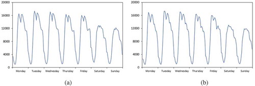
The region within the 6th Ring Road in Beijing was selected as the research area. The GPS traces of 3,300 taxis in Beijing from 1 to 28 December 2015 were collected. The statuses of taxis, including ID, position, timestamp, and whether the taxi was occupied by passengers or not, were sampled every minute for 24 h. After filtering out invalid points and trips, a total of 1.07 million pick-up and drop-off pairs in the research area were obtained. The research area was partitioned with 1 km × 1 km regular grid, and then taxi pick-ups and drop-offs were spatially allocated to corresponding grid cells. The total number of pick-ups and drop-offs in each grid cell is spatially distributed as shown in Figure 2. The series of pick-ups and drop-offs are periodic, so the hourly quantities are averaged into one week period in each grid cell. As a result, the spatio-temporal series data sets about taxi mobility were constructed. The temporal variance is shown in Figure 3.

Figure 2. Spatial distribution of (a) pick-ups and (b) drop-offs.

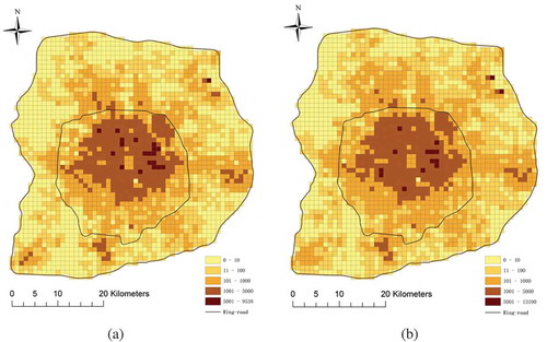
Figure 3. Temporal variance per week of (a) pick-ups and (b) drop-offs.

3.2. Results

We constructed two spatio-temporal data sets by taxi pick-ups and drop-offs for evaluating the spatio-temporal autocorrelation index. In each grid cell, the observed variable is a time series of the hourly number of pick-ups or drop-offs that is averaged in one week. We performed the proposed measurement upon the two data sets to interpret the global and local spatial patterns of the temporal taxi travel. The spatial weight matrix is generated by the inverse distance square between any two grid cells, and then is row-standardized.

The global spatial patterns are measured by the spatio-temporal index from the time series pick-ups and drop-offs. The global autocorrelation coefficient of pick-ups is 0.507 with z-score equal to 141.22 and p-value less than 0.01; the global coefficient of drop-offs is 0.369 with z-score equal to102.78 and p-value less than 0.01. This reveals a global pattern of taxi travel. The spatio-temporal autocorrelation of taxi travel is significantly strong in Beijing, and pick-ups are more spatiotemporally autocorrelated than drop-offs. The arrivals of taxi passengers are more disperse in space and time than departures. These results are consistent to the common sense about human mobility in big cities.

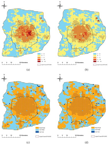
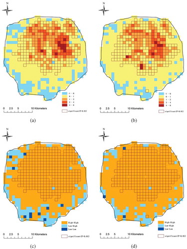
The local patterns are measured by the spatio-temporal LISA index based on the pick-up and drop-off sequences in each grid cell. The distributions of LISA and spatial patterns are shown in Figure 4. There is strong positive spatio-temporal autocorrelation within the 5th Ring Road, weak negative spatio-temporal autocorrelation nearby the 6th Ring Road, and almost no spatio-temporal autocorrelation between the 5th and 6th Ring Roads. Almost all areas within the 5th Ring Road exhibit a significant High-High autocorrelation pattern. These areas, considered urban areas in Beijing, are densely populated. More taxis and passengers result in much more traffic flow than normal. Near locations are more likely to have similar travel volume and rhythm, thus they are likely to usher in traffic peaks during similar time periods. The spatial autocorrelation is not significant outside the 5th Ring Road. Low population density and diverse land use in these urban fringes results in lower and less regular taxi travel.

Figure 4. Spatio-temporal LISA within the 6th Ring Road. (a) Distribution of the LISA of pick-ups. (b) Distribution of the LISA of drop-offs. (c) Spatial pattern of pick-ups. (d) Spatial pattern of drop-offs.

We narrowed the study area to the region within the 5th Ring Road for investigating the finer spatial patterns in the city center. The global autocorrelation coefficients of pick-ups and drop-offs within the 5th Ring Road are 0.681 with z-score equal to 87.6 and 0.639 with z-score equal to 82.3, respectively, under the 0.01 significance level. The spatio-temporal autocorrelation of taxi travel within the 5th Ring Road is stronger than that outside, and the pick-ups and drop-offs exhibit similar spatio-temporal patterns.

The distributions of LISA and spatial patterns within the 5th Ring Road are shown in Figure 5. The closer to the city center, the stronger the positive correlation is. Almost all areas within the 5th Ring Road exhibit a significant High-High autocorrelation pattern. The margin areas are Low-High type, where the travel patterns were diverse. The areas around Beijing Railway Station, Beijing West Railway Station, Beijing South Railway Station, and CBD have the strongest correlation because of the large quantity of taxi-passengers and continuous traffic flows. The followings are some important commercial and office areas including Zhongguancun, Xidan, Wangjing SOHO, Financial Street, and so on. The temporal variances of taxi travel in these areas are much similar to their neighbors, with almost the same rush hours for commuting. The cold spots which belong to the Low-High pattern are inside some large parks or areas where taxies can barely drive, including Summer Palace, Yuanmingyuan Park, Olympic Park, Chaoyang Park, Temple of Heaven Park, and the Nanyuan Airport.

Figure 5. Spatio-temporal LISA within the 5th Ring Road. (a) Distribution of the LISA of pick-ups. (b) Distribution of the LISA of drop-offs. (c) Spatial pattern of pick-ups. (d) Spatial pattern of drop-offs.

4. Discussion

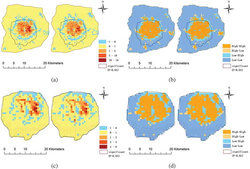
To evaluate the effectiveness of the spatio-temporal autocorrelation measurement, we compared the results with those of the classical Moran’s I and LISA indexes. After averaging the number of pick-ups and drop-offs by day, in each grid cell, we measured their classical spatial autocorrelation. The global autocorrelation coefficients of pick-ups and drop-offs were compared with the results of the spatio-temporal autocorrelation measurement, as shown in Table 1. The autocorrelation measured by the proposed method were stronger and more significant than those measured by the classical method, especially within the 5th Ring Road in Beijing. The temporal variances enlarged the spatial autocorrelation.

Table 1. Comparation of the spatio-temporal autocorrelation measurement and the classical measurement.

		pick-ups		drop-offs
region	autocorrelation measurement	I	z-score	I	z-score
6th Ring Road	spatio-temporal	0.507**	141.22	0.369**	102.78
	classical	0.431**	120.2	0.406**	113.2
5th Ring Road	spatio-temporal	0.681**	87.6	0.639**	82.3
	classical	0.424*	54.7	0.404*	52.1

* 0.1 significance level; ** 0.01 significance level.

The distributions of LISA and spatial patterns obtained by the classical measurement are shown in Figure 6. Compared to the patterns in Figures 4 and 5, the spatial patterns discovered by the classical method are less significant. Within both research areas, the results of the two methods represent similar distribution. However, the spatio-temporal LISA can recognize finer patterns than the classical index. The spatio-temporal LISA values are more distinguished at different locations, and more Low-Low patterns are discovered. In addition, The spatio-temporal measurement produces significant results at more locations than the classical index.

Figure 6. Classical LISA. (a) Distribution of the LISA of pick-ups and drop-offs within the 6th Ring Road. (b) Spatial pattern of pick-ups and drop-offs within the 6th Ring Road. (c) Distribution of the LISA of pick-ups and drop-offs within the 5th Ring Road. (d) Spatial pattern of pick-ups and drop-offs within the 5th Ring Road.

5. Conclusions

We proposed a spatio-temporal autocorrelation measurement by extending the classical Moran’s I and LISA indexes for time series data of collective human mobility. The new method integrates both the temporal variance and the value deviation at a location to reveal the spatial pattern. Analyzing taxi rides data in Beijing in this experiment, the method exhibited a good ability to discover global and local spatio-temporal pattern of taxi travel. It can reveal spatial autocorrelation and heterogeneity in collective human mobility. This method and the research results are useful for understanding human mobility and urban structures.

Additional information

Funding

This work is funded by the National Natural Science Foundation of China [grant numbers 41830645 and 41625003].

Notes on contributors

Yong Gao

Yong Gao received his Ph.D. in Geographic Information Science from Peking University, China. He is currently an associate professor at the Institute of Remote Sensing and Geographic Information System, Peking University. His research interests are in spatial data mining and geographic information science.

Jing Cheng

Jing Cheng received her M.S. degree at the Institute of Remote Sensing and Geographic Information System, Peking University. Her research interest is spatial data analysis.

Haohan Meng

Haohan Meng received his B.S. degree at the School of Earth and Space Sciences, Peking University. He is now an M.S. student at the Institute of Remote Sensing and Geographic Information System, Peking University. His research interests include spatial data analysis and geographic Information science.

Yu Liu

Yu Liu received his Ph.D. degree from Peking University. He is currently a professor of GIScience at the Institute of Remote Sensing and Geographic Information System, Peking University. His research interest mainly concentrates in humanities and social sciences based on big geo-data.

References

- Anselin, L. 1995. “Local Indicators of Spatial Association—LISA.” Geographical Analysis 27 (2): 93‒115.
- Anselin, L., I. Syabri, and O. Smirnov. 2002. “Visualizing Multivariate Spatial Correlation with Dynamically Linked Windows.” In “New Tools in Spatial Data Analysis.” Proceedings of a Workshop. Center for Spatially Integrated Social Science, University of California, edited by L. Anselin and S. Rey, Santa Barbara: CDROM.
- Chouakria, A. D., and P. N. Nagabhushan. 2007. “Adaptive Dissimilarity Index for Measuring Time Series Proximity.” Advances in Data Analysis and Classification 1 (1): 5‒21. doi:10.1007/s11634-006-0004-6.
- Dubé, J., and D. Legros. 2013. “A Spatio-Temporal Measure of Spatial Dependence: An Example Using Real Estate Data.” Papers in Regional Science 92 (1): 19‒30.
- Geary, R. C. 1954. “The Contiguity Ratio and Statistical Mapping.” The Incorporated Statistician 5 (3): 115‒145. doi:10.2307/2986645.
- Jiang, B., J. Yin, and S. Zhao. 2009. “Characterizing the Human Mobility Pattern in a Large Street Network.” Physical Review E 80 (2): 021136. doi:10.1103/PhysRevE.80.021136.
- Lee, J., and S. Li. 2017. “Extending Moran’s Index for Measuring Spatiotemporal Clustering of Geographic Events.” Geographical Analysis 49 (1): 36‒57. doi:10.1111/gean.2017.49.issue-1.
- Liu, X., L. Gong, Y. Gong, and Y. Liu. 2015. “Revealing Travel Patterns and City Structure with Taxi Trip Data.” Journal of Transport Geography 43: 78‒90. doi:10.1016/j.jtrangeo.2015.01.016.
- Liu, Y., C. Kang, S. Gao, Y. Xiao, and Y. Tian. 2012a. “Understanding Intra-Urban Trip Patterns from Taxi Trajectory Data.” Journal of Geographical Systems 14 (4): 463‒483. doi:10.1007/s10109-012-0166-z.
- Liu, Y., D. Tong, and X. Liu. 2015. “Measuring Spatial Autocorrelation of Vectors.” Geographical Analysis 47 (3): 300‒319. doi:10.1111/gean.12069.
- Liu, Y., F. Wang, Y. Xiao, and S. Gao. 2012b. “Urban Land Uses and Traffic ‘Source-Sink Areas’: Evidence from GPS-Enabled Taxi Data in Shanghai.” Landscape Urban Plan 106 (1): 73–87. doi:10.1016/j.landurbplan.2012.02.012.
- Moran, P. A. 1950. “Notes on Continuous Stochastic Phenomena.” Biometrika 37 (1/2): 17‒23. doi:10.1093/biomet/37.1-2.17.
- Ord, J. K., and A. Getis. 1995. “Local Spatial Autocorrelation Statistics: Distributional Issues and an Application.” Geographical Analysis 27 (4): 286‒306.
- Pei, T., S. Sobolevsky, C. Ratti, S. Shaw, T. Li, and C. Zhou. 2014. “A New Insight into Land Use Classification Based on Aggregated Mobile Phone Data.” International Journal of Geographical Information Science 28 (9): 1988‒2007. doi:10.1080/13658816.2014.913794.
- Porat, I., M. Shoshany, and A. Frenkel. 2012. “Two Phase Temporal-Spatial Autocorrelation of Urban Patterns: Revealing Focal Areas of Re-Urbanization in Tel Aviv-Yafo.” Applied Spatial Analysis and Policy 5 (2): 137‒155. doi:10.1007/s12061-011-9065-9.
- Tobler, W. R. 1970. “A Computer Movie Simulating Urban Growth in the Detroit Region.” Economic Geography 46 (sup1): 234‒240. doi:10.2307/143141.
- Wu, L., X. Cheng, C. Kang, D. Zhu, Z. Huang, and Y. Liu. 2018. “A Framework for Mixed-Use Decomposition Based on Temporal Activity Signatures Extracted from Big Geo-Data.” International Journal of Digital Earth. (online published). doi: 10.1080/17538947.2018.1556353.
- Zhi, Y., H. Li, D. Wang, M. Deng, S. Wang, J. Gao, Z. Duan, and Y. Liu. 2016. “Latent Spatio-Temporal Activity Structures: A New Approach to Inferring Intra-Urban Functional Regions via Social Media Check-in Data.” Geo-spatial Information Science 19 (2): 94‒105. doi:10.1080/10095020.2016.1176723.
- Zhu, X., and D. Guo. 2017. “Urban Event Detection with Big Data of Taxi OD Trips: A Time Series Decomposition Approach.” Transactions in GIS 21: 560‒574. doi:10.1111/tgis.2017.21.issue-3.