Analysis of mobility data – A focus on Mobile Mapping Systems

ABSTRACT

The increasing availability of devices to capture the position of moving objects (and other environmental information) leads to a very large amount and variety of mobility data. In order to obtain important information about the objects, their behavior or the environment of the objects, an automatic analysis is required. This article highlights current research questions in the context of the analysis of mobility data and presents them on the basis of work carried out at the Institute of Cartography and Geoinformatics (ikg) at Leibniz University of Hannover, Germany. A focus is put on the analysis and exploitation of information from Mobile Mapping vehicles.

KEYWORDS:

• Trajectories
• Lidar data
• automatic analysis
• traffic applications

1. Introduction and overview

Mobile data is typically available in the form of so-called trajectories, i.e. sequences of individual 2D or 3D points with time stamps. In this way, for example, the traveled path of a hiker can be documented, the movement of a bird or a football player. The trajectories are recorded by GPS sensors or by observation and object tracking with cameras. In addition to the pure recording of the trajectory, additional information can be captured by additional sensors. A prominent example of this are so-called mobile mapping vehicles, which usually consist of a high-precision positioning unit, which capture the trajectories, but also the orientation information, and comprise additional sensors: e.g. Laser scanners and cameras. In the context of the processing of mobility data, a number of interesting and complex questions arise, among others:

• Alignement and fusion of the data: measurements at different times or measurements with different sensors result in large, redundant data sets of the environment, which have to be aligned and integrated.

• Interpretation of environmental information to determine the dynamics of objects in the environment

• Interpretation of motion data to determine behavior

In the following, these questions will be dealt with briefly and illustrated. The methods used in the works are only briefly sketched, more details can be found in the refered papers – together with a detailed description of the state of the art.

2. Acquisition of environmental information

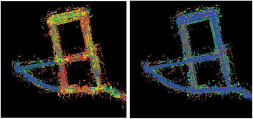
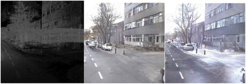
The ikg’s Mobile Mapping System uses the laser scanner to capture potentially 600,000 3D points per second, plus images from the four cameras that look in different directions. The accuracy of a single laser measurement is 2 cm. The positioning and orientation of the vehicle is carried out by means of a highly accurate GPS-IMU (Inertial Measurement Unit). In highly dynamic situations (flowing traffic, normal speeds), absolute positioning accuracies of approx. 20 cm can be achieved. These accuracies are already sufficient for many questions and applications. If, on the other hand, changes in the environment are to be detected, measurement runs acquired at different points in time must be superimposed and analyzed as precisely as possible. The mentioned inaccuracies in the range of 20 cm lead to difficulties in the identification and analysis of real changes. Therefore, a method was developed at the ikg which is able to merge different scan run data. This is carried out by a global optimization approach, in which the trajectory is adapted on the basis of stable objects in the object space in such a way that related points from different measurement runs fit together optimally. The global optimization of potentially very large data sets can be achieved by decomposing the problem and calculating it in a Hadoop framework (Brenner 2016). Figure 1 shows the superposition of two data sets that were recorded one year apart. The deviations of the points before the adjustment are about 20 cm, afterwards about 2 cm. In the adjustment 304,748,078 points were processed and 21,300 unknowns (= 7.1 km trajectory) were determined.

Figure 1. Comparison of the points before and after the adjustment: deviations before and after the adjustment are approx. 20 cm, afterwards 2 cm (red: 20 cm – blue: 2 cm).

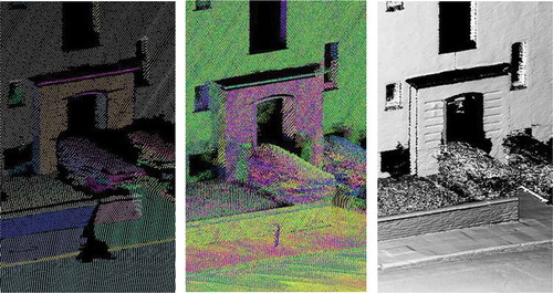
After the adjustment, high-density and high-precision point clouds can be generated (see Figure 2). It is very nice to see how much detail is visible in the data: masonry, pavement, as well as the road condition.

Figure 2. Left: Image of a scan run; middle: simple superposition of several scan runs; right: result of the fusion.

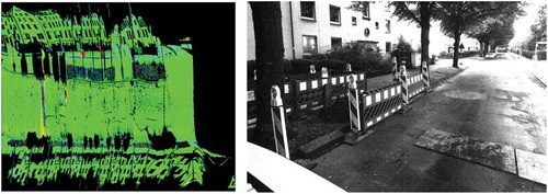
In addition, changes between the measurement runs can be recorded precisely. This is shown in Figure 3: relevant changes in the range greater than 2 cm are shown in red or blue. Noisy changes can be seen in the vegetation; larger deviations indicate structural changes such as a construction site.

Figure 3. (Left) in red and blue changes can be seen between the images, e.g. the blue stripe on the street stands for an iron slab that was laid in the course of a construction site (right).

In the context of this research, further questions arise which are dealt with in doctoral theses at ikg, for example the use of suitable environmental information (stable objects such as facades, posts) for autonomous driving (Schlichting and Brenner 2016), and the automatic classification of changes (change types, frequencies) (Schachtschneider, Schlichting, and Brenner 2017). In this work, biweekly measurements of a 12 km route were acquired (Lidar, camera-data), leading to a rich data set comprising information about the environment at different seasons, weekdays and times of the day. This information has been exploited in another research work to synthesize realistic visualizations from Lidar data projections. In order to do so, a conditional GAN was trained with pairs of Lidar and camera-data, including a time-stamp (Peters and Brenner 2018). In this way it is possible to not only generate realistic views (Figure 4), but also realistic views at different times of the year, e.g. winter-summer visualizations of the same scene (Figure 5).

Figure 4. (Left) lidar projection, (right) camera image, (middle) synthesized image.

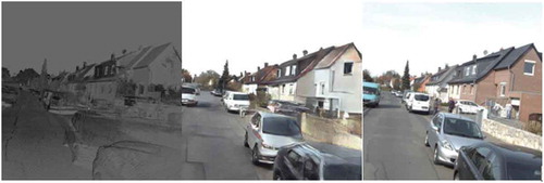
Figure 5. (Left) lidar projection, (middle) summer view, (right) winter view.

3. Dynamic parking maps by crowd sensing

An important requirement in the context of autonomous driving is to record the dynamics of the environment in future maps. This makes it possible for the autonomous vehicle to have an “expectation” about its environment and thus to compare its sensor readings more easily and reliably with the map data. In this context, a dissertation examined how the dynamics of car park occupancy can be recorded and analyzed (Bock, Eggert, and Sester 2015). In a measurement campaign, 11 journeys on the same route were undertaken on one day. In the recorded 3D point clouds, vehicles were automatically classified and detected using machine learning methods and the occupancy during the course of the day was analyzed. Figure 6 shows the process of capturing, segmenting and classifying the point cloud, as well as the resulting car park occupancy map.

Figure 6. Sequence: point cloud – segmentation of the point cloud into coherent units – classification of the units into cars and extraction of the cars – occupancy map.

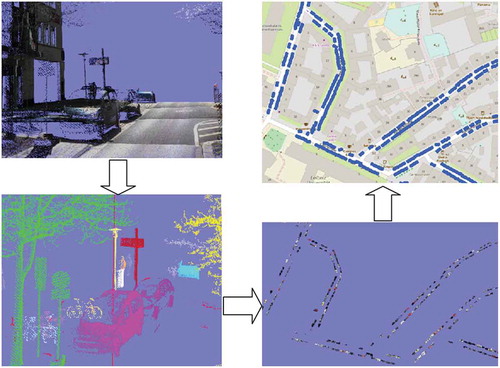
From this, typical car park occupancy patterns can be determined, which are shown in Figure 7.

Figure 7. Occupancy of parking spaces during the day.

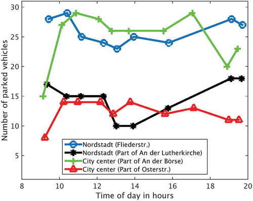
It becomes clear that in the city center (green, red) there is an increase in the number of occupied parking spaces in the morning, which decreases towards the evening. In the residential area (Nordstadt), on the other hand, the opposite is true.

The dissertation showed that the parking dynamics can be measured by crowd sensing, i.e. the standard sensors of future vehicles. For example, it has been proven that taxis in San Francisco can map parking behavior very well, which also makes it possible to make more precise forecasts of the availability of parking spaces (Bock and Di Martino 2017).

4. Determination of movement behavior of mobile objects

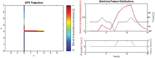
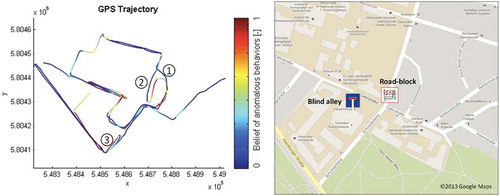
Motion trajectories allow inferences about the underlying behavior of the moving object. A study at ikg investigated to what extent it can be deduced from a vehicle trajectory whether the driver shows a typical, normal behavior or whether his behavior is unusual and indicates that he may have lost his way and needs help. The approach of Huang et al. uses a Bayesian approach to detect abnormal behavior (Huang, Zhang, and Sester 2014). The basic idea is that an insecure driver will show different behavioral patterns, such as wrong turns, detours, driving the same route again. The approach therefore describes the unusual behavior as a composition of three elements: 1. (dense sequence of) turns, 2. detours, and 3. route repetition. These characteristics are extracted from the trajectories and analyzed using a Markov model. Figure 8 shows a trajectory on the left that was traversed from bottom to top. The color indicates how high the confidence in unusual behavior is. Abnormal behavior is assumed as soon as the road user drives the same route again.

Figure 8. Trust (belief) in anomalous behavior on the route from bottom to top (left).

In addition to analyzing individual trajectories, it is also possible to analyze collective behavior and draw conclusions from it: if many road users show similar, unusual behavior, this may be an indication of a disturbance in traffic. This can be seen in Figure 9, where a roadblock leads to unusual behavior in the environment.

Figure 9. Example of collective behavior to detect a blocked road.

5. Creating a hazard map and its use for autonomous vehicles

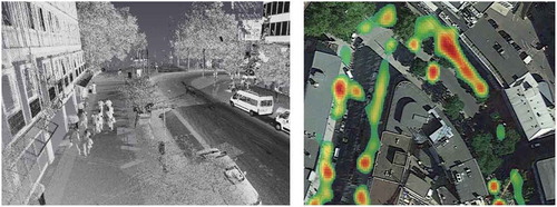
As explained above, autonomous vehicles need precise maps of their environment to navigate within. In addition, additional information is needed to help the vehicle understand the situations it may face. This can be achieved by means of so-called behavior maps or hazard maps (Busch, Schlichting, and Brenner 2017). These maps mark areas in which certain phenomena can be expected: for example, an area in which a low sun can dazzle at sunrise or sunset, or an area in which pedestrians often cross the road abruptly. The latter can be determined using data from the Mobile Mapping System. For this purpose, an object classification of the 3D point clouds was first carried out, similar to the project with the parking lot maps, but pedestrians were determined in the process. From the superposition of the positions of pedestrians at different times, so-called heat maps can be derived, which show frequent occurrences (Figure 10, right).

Figure 10. Pedestrians are depicted in the point clouds (left); these are automatically classified and data from many scans are aggregated to heat maps (right).

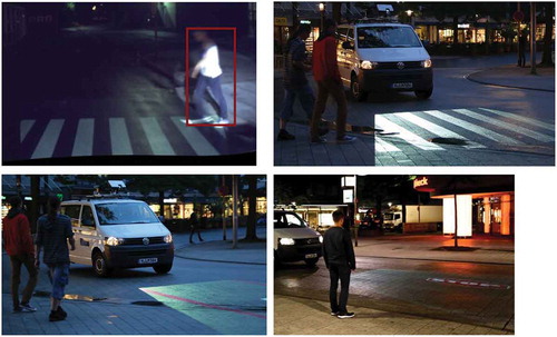
This information can be used by an autonomous vehicle to search specifically for persons in these areas (cf. Figure 11, top left). If these are identified, it is of great importance for future autonomous systems that they can communicate their planned behavior to pedestrians. In a prototypical realization, a LCD-projector was placed on top of the mobile mapping vehicle of the ikg, which visually communicates to pedestrians whether the vehicle intending to stop or to continue. In the first case it projects a zebra crossing onto the road, in the second case a stop sign (Figure 11, bottom).

Figure 11. Identification of a pedestrian – projection of a zebra strip (top) projection of a red lane edge and a stop sign indicates that the vehicle will not stop (bottom).

6. Summary

The work presented here is intended to illustrate by way of examples which tasks arise in the context of the automatic collection and analysis of mobility data and which fields of application they can be used for. Of great importance are, on the one hand, methods of machine learning, which are used for a variety of interpretation tasks. On the other hand, the scalable processing of very large, heterogeneous data sets (big data) is becoming increasingly important (Li et al. 2015).

Additional information

Funding

This work is supported by funds from the German Research Foundation (DFG) in the Research Training Groups SocialCars and i.c.sens.

Notes on contributors

Monika Sester

Monika Sester is an full professor at Leibniz University Hanover. She received her PhD and her habilitation from the University of Stuttgart. Her research interests are the automation of spatial data analysis, applied to many fields, e.g. data interpretation, generalization and fusion.

References

- Bock, F., and S. Di Martino. 2017. “How Many Probe Vehicles Do We Need to Collect On-street Parking Information?” 5th IEEE International Conference on Models and Technologies for Intelligent Transportation Systems (MT-ITS), Las palmas, Spain, 538–543. doi:10.1142/S021881041772042X.
- Bock, F., D. Eggert, and M. Sester. 2015. “On-street Parking Statistics Using LiDAR Mobile Mapping, Intelligent Transportation Systems (ITSC).” 2015 IEEE 18th International Conference on, Naples, Italy, June 26–28, 2812–2818.
- Brenner, C. 2016. “Scalable Estimation of Precision Maps in a MapReduce Framework.” Proceedings of the 24th ACM SIGSPATIAL International Conference on Advances in Geographic Information Systems, New York, NY, USA, 27: 1–27:10.
- Busch, S., A. Schlichting, and C. Brenner. 2017. “Generation and Communication of Dynamic Maps Using Light Projection.” Proceedings, 28th International Cartographic Conference: ICC 2017, Washington, D.C., USA, July 2–7.
- Huang, H., L. Zhang, and M. Sester. 2014. “A Recursive Bayesian Filter for Anomalous Behavior Detection in Trajectory Data.” Proceedings of AGILE, Connecting a Digital Europe through Location and Place, edited by Huerta, J., S. Sven, and G. Carlos, 91–104. Cham: Springer International Publishing.
- Li, S., S. Dragicevic, F. A. Castro, M. Sester, S. Winter, A. Coltekin, C. H. Pettit, et al. 2015. “Geospatial Big Data Handling Theory and Methods: A Review and Research Challenges.” ISPRS Journal of Photogrammetry and Remote Sensing 115: 119–133. doi:10.1016/j.isprsjprs.2015.10.012.
- Peters, T., and C. Brenner. 2018. “Conditional Adversarial Networks for Multimodal Photo-Realistic Point Cloud Rendering.” Spatial Big Data and Machine Learning in GIScience, GIScience Workshop 2018, Melbourne, Australia.
- Schachtschneider, J., A. Schlichting, and C. Brenner. 2017. “Assessing Temporal Behaviour in Lidar Point Clouds of Urban Environments.” International Archives of the Photogrammetry, Remote Sensing & Spatial Information Sciences 42: 543–550.
- Schlichting, A., and C. Brenner. 2016. “Vehicle Localization by LIDAR Point Correlation Improved by Change Detection.” ISPRS-International Archives of the Photogrammetry, Remote Sensing and Spatial Information Sciences XLI-B1: 703–710. doi:10.5194/isprsarchives-XLI-B1-703-2016.