Crop type mapping using LiDAR, Sentinel-2 and aerial imagery with machine learning algorithms

ABSTRACT

LiDAR data are becoming increasingly available, which has opened up many new applications. One such application is crop type mapping. Accurate crop type maps are critical for monitoring water use, estimating harvests and in precision agriculture. The traditional approach to obtaining maps of cultivated fields is by manually digitizing the fields from satellite or aerial imagery and then assigning crop type labels to each field – often informed by data collected during ground and aerial surveys. However, manual digitizing and labeling is time-consuming, expensive and subject to human error. Automated remote sensing methods is a cost-effective alternative, with machine learning gaining popularity for classifying crop types. This study evaluated the use of LiDAR data, Sentinel-2 imagery, aerial imagery and machine learning for differentiating five crop types in an intensively cultivated area. Different combinations of the three datasets were evaluated along with ten machine learning. The classification results were interpreted by comparing overall accuracies, kappa, standard deviation and f-score. It was found that LiDAR data successfully differentiated between different crop types, with XGBoost providing the highest overall accuracy of 87.8%. Furthermore, the crop type maps produced using the LiDAR data were in general agreement with those obtained by using Sentinel-2 data, with LiDAR obtaining a mean overall accuracy of 84.3% and Sentinel-2 a mean overall accuracy of 83.6%. However, the combination of all three datasets proved to be the most effective at differentiating between the crop types, with RF providing the highest overall accuracy of 94.4%. These findings provide a foundation for selecting the appropriate combination of remotely sensed data sources and machine learning algorithms for operational crop type mapping.

KEYWORDS:

• LiDAR
• multispectral imagery
• sentinel-2
• machine learning
• crop type classification
• per-pixel classification

1. Introduction

Remotely sensed data acquired by satellites or aircraft (manned and unmanned) are frequently used for generating crop type maps (Pádua et al. 2017), with multispectral sensors mounted on satellites being the most popular. Examples of satellite imagery used for crop type mapping include those acquired by SPOT 4 and 5 (Turker and Kok 2013; Turker and Ozdarici 2011), Landsat 8 (Gilbertson, Kemp, and Van Niekerk 2017; Liaqat et al. 2017; Siachalou, Mallinis, and Tsakiri-Strati 2015), Quickbird (Senthilnath et al. 2016; Turker and Ozdarici 2011), RapidEye (Siachalou, Mallinis, and Tsakiri-Strati 2015), and MODIS (Dell’Acqua et al. 2018; Liaqat et al. 2017). Aerial multispectral sensors are also frequently employed, especially if very high spatial resolution imagery is required (Rajan and Maas 2009; Mattupalli et al. 2018; Wu et al. 2017; Vega et al. 2015). Fewer examples of the use of hyperspectral imagery are available (Jahan and Awrangjeb 2017; Liu and Yanchen 2015; Yang et al. 2013), mainly due to the expense in obtaining such data. Similarly, the use of LiDAR data for crop type mapping is uncommon, with Mathews and Jensen (2012) and Estrada et al. (2017) being notable exceptions.

LiDAR data are becoming increasingly available as more aerial surveys are carried out and Earth observation satellites fitted with LiDAR sensors are launched. For instance, the recent launch of the ICESat-2 LiDAR satellite (September 2018) and the attachment of the GEDI LiDAR sensor to the international space station (December 2018) has opened up many new avenues for research and will provide the first opportunity to map vegetation structure at global scale and at high resolutions (Escobar and Brown 2014). Small factor LiDAR sensors mountable on unmanned aerial vehicles (UAV) will also contribute to increased data availability. These new sources of LiDAR data bode well for the agricultural sector (Sankey et al. 2017) as it will be invaluable for crop type classifications, especially when combined with high resolution, multispectral and multi-temporal optical images such as those provided by the Sentinel-2 constellation. The two Sentinel-2 satellites carry 13-band multispectral sensors with swath widths of 290 km and resolutions of 10 m, 20 m and 60 m, depending on the wavelength, which is ideal for crop type mapping.

Machine learning has been widely used in remote sensing (Lary et al. 2016). Non-parametric machine learning algorithms are capable of dealing with high-dimensional datasets with non-normal distributed data (Al-doski et al. 2013; Gilbertson, Kemp, and Van Niekerk 2017). Commonly used machine learning algorithms are Decision Trees (DTs), Random Forest (RF), Neural Network (NN), and Support Vector Machines (SVM) (Al-doski et al. 2013; Lary et al. 2016). Given that the Sentinel-2 satellites have been in operation for a relatively short time (since 2015), the number of studies that have used the data for crop type classifications are limited. The combination of this data with machine learning algorithms is particularly scarce. However, three studies, namely Inglada et al. (2015), Matton et al. (2015), and Valero et al. (2016), used SPOT 4-Take 5 and Landsat 8 data to emulate Sentinel-2 data. The studies used machine learning classifiers to create crop type maps with Inglada et al. (2015) using RF and SVM, Matton et al. (2015) applying Maximum Likelihood (ML) and K-means, and Valero et al. (2016) applying the RF classifier. Inglada et al. (2015) and Valero et al. (2016) both created crop type maps for 12 sites, each in a different country. Inglada et al. (2015) obtained overall accuracies of above 80% for seven of the sites while three of the sites had accuracies of between 50% and 70%. Valero et al. (2016) achieved accuracies of around 80%. Matton et al. (2015) considered eight sites, each in a different country, and obtained accuracies of above 75% for all sites, except in one where an accuracy of 65% was achieved. Two studies, Immitzer, Vuolo, and Atzberger (2016) and Estrada et al. (2017), classified crops using Sentinel-2 data with the former using RF to classify seven crop types and the latter using DTs to classify five crop types. Immitzer, Vuolo, and Atzberger (2016) compared an Object-Based Image Analysis (OBIA) and a per-pixel approach, with OBIA obtaining an Overall Accuracy (OA) of 76.8% and the per-pixel classification obtaining an OA of 83.2%. Estrada et al. (2017) considered two study areas and obtained OAs of 85.6% and 95.6% respectively.

Aerial imagery is obtained from sensors mounted on either a piloted (manned) aircraft or a UAV (Matese et al. 2015). An UAV has the benefit of a low operational cost, but is limited to short flight times that limit the area that can be surveyed (Matese et al. 2015). Vega et al. (2015) used ML to classify two crop types (sunflowers and non-sunflowers) using multispectral UAV imagery as input. Three resolutions (0.01 m, 0.3 m and 1 m) were evaluated. OAs of above 85% were obtained at all three resolutions (Vega et al. 2015). Wu et al. (2017) performed an OBIA SVM and a per-pixel ML classification on 0.4 m multispectral UAV imagery. They achieved an OA of 95% for the object-based SVM classification and the per-pixel ML classification obtained an OA of 75% when the multispectral imagery was used (Wu et al. 2017). Mattupalli et al. (2018) tested imagery from two different sensors, with the first sensor mounted on a UAV and the second mounted on a manned aircraft. The imagery from the two sensors were resampled to 0.1 m and then used as input to ML to classify three crop types. The OAs achieved ranged from 89.6% to 98.1% with the imagery from the manned aircraft achieving outperforming the UAV imagery.

Several studies have combined aerial and satellite imagery with height data to improve crop type and other land cover classifications. Height data can be obtained using stereo photogrammetry techniques or by using LiDAR data. Stereo photogrammetry uses overlapping images to create a Digital Surface Model (DSM) (Wu et al. 2017). LiDAR is a form of active remote sensing that captures 3D point clouds of the earth’s surface by transmitting and receiving energy pulses in a narrow range of frequencies (Campbell and Wynne 2011; Ismail et al. 2016). LiDAR is commonly used to derive surface height information by either using the 3D point cloud or by interpolating a DSM or digital terrain model (DTM) (Zhou 2013). A Normalized DSM (nDSM), or Canopy Height Model (CHM), can be created by subtracting the DSM from the DTM. LiDAR has an advantage over photogrammetric methods in that LiDAR generally provides more accurate height measurements compared to photogrammetric methods, especially for areas with dense vegetation (Satale and Kulkarni 2003). In addition, LiDAR is less affected by weather conditions compared to photogrammetric methods (Satale and Kulkarni 2003). LiDAR can also penetrate vegetation canopies and obtain height information of the terrain below. The terrain heights can then be used to create a DTM and nDSM with higher accuracy and less effort than with photogrammetric methods. Besides height information, LiDAR can also provide returned intensity information, which can be used to discriminate between different land covers. For instance, water results in low intensity returns, while the intensity of returns from vegetation is high (Antonarakis, Richards, and Brasington 2008).

The majority of the studies that use LiDAR data for classification derived an nDSM or CHM as they represent only the aboveground features (Yan, Shaker, and El-Ashmawy 2015). Chen et al. (2009) combined Very High Resolution (VHR) Quickbird imagery with LiDAR data to classify land cover in an urban setting. The OA increased from 69.1% to 89.4% when the LiDAR derived nDSM was used and added to the imagery as input to the classifier (Chen et al. 2009). They attributed the increase in accuracy to the height data, which made it easier to differentiate between land covers that have similar spectral signatures. Wu et al. (2017) derived an orthomosaic and a DSM from aerial imagery to classify crop types and obtained an overall increase in OA of 3% when the DSM was used along with the orthomosaics. Estrada et al. (2017) classified a LiDAR point cloud, which was used in an interpolation procedure to produce a rasterized elevation model. The latter was then combined with Sentinel-2 imagery to classify crops. However, unlike Chen et al. (2009) and Wu et al. (2017) who combined the LiDAR data with imagery as input features to the classifiers, Estrada (2017) classified the LiDAR and Sentinel-2 data separately and then combined the results using a post-classification aggregation procedure.

Liu and Yanchen (2015) classified crops using airborne hyperspectral and a LiDAR derived CHM. They compared five different classification schemes, using SVM as classifier in an OBIA environment. The OA increased by 8.2% when VHR hyperspectral data was combined with CHM and 9.2% when the CHM was combined with Minimum Noise Fraction transformed (MNF) hyperspectral data (Liu and Yanchen 2015). The highest OA (90.3%) was achieved when the geometric properties of objects and image textures (that were applied on the CHM) were combined with the untransformed CHM and MNF data. This increase was attributed to the ability of image textures to quantify the structural arrangements of objects and their relationship to the environment. They thus provide supplementary information related to the variability of land cover classes and can be used to discriminate between heterogeneous crop-fields (Chica-Olmo and Abarca-Hernández 2000; Peña-Barragán et al. 2011; Zhang and Zhu 2011). Jahan and Awrangjeb (2017) used hyperspectral imagery and a LiDAR-derived DSM, nDSM and intensity raster to classify five land covers. Their study considered two machine learning classifiers (SVM and DTs) and tested nine different combinations of the hyperspectral and LiDAR data. They found that, for the SVM experiments, OA increased by 7.6% when the DSM was added to the hyperspectral data and by 8.4% when image textures (performed on the DSM) were added. Similar but more modest increases (3% and 4.3% respectively) were observed for the DT experiments.

Although several studies have combined LiDAR data with imagery to classify land cover and crop types, very little work has been done on using LiDAR data on its own for this purpose. A notable exception is Brennan and Webster (2006) who used four LiDAR derivatives (intensity, multiple return, normalized DSM and a DSM) to classify land cover and obtained an OA of 94.3% when targeting ten land cover classes and 98.1% when targeting seven classes. Charaniya, Manduchi, and Lodha (2004) classified four land covers using four LiDAR derivatives (normalized DSM, height variation, multiple returns and intensity) and obtained an OA of 85%. Also using LiDAR derivatives, Mathews and Jensen (2012) obtained an OA of 98.2% when differentiating vineyards from other land covers.

From the literature, it seems that the use of LiDAR data as additional input variables (along with imagery) improves land cover classifications. It is even possible to extract individual crop types (e.g. wine grapes) using LiDAR derivatives only, i.e. without using optical imagery as additional input data to classification algorithms. However, it is not clear what value LiDAR data provide to differentiate different types of crops – when used on its own and when it is combined with satellite and aerial imagery. This study investigates the performance of various machine learning algorithms on different combinations of multispectral and LiDAR data for crop type mapping in Vaalharts (Prins 2019), the largest irrigation scheme in South Africa. To our knowledge, no study has assessed the use of LiDAR data on its own for differentiating multiple crop types. Given that LiDAR data are becoming increasingly available at regional scales – and the likelihood that data from space borne LiDAR (e.g. GEDI, IceSat-2) will soon become common – an improved understanding of the value of such data for crop type classification is needed. The crop type maps produced using LiDAR data are compared to crop type maps that were produced using 20 cm aerial and 10 m Sentinel-2 imagery. In addition, the LiDAR data are used in different combinations with the Sentinel-2 and aerial imagery as input to the machine learning classifiers. Ten machine learning classification algorithms, namely RF, DTs, Extreme Gradient Boosting (XGBoost), K-Nearest Neighbor (k-NN), Logistic Regression (LR), Naïve Bayes (NB), NN, Deep Neural Network (d-NN), SVM with a Linear kernel (SVM-L), and SVM with a Radial Basis Function kernel (SVM RBF), are used to determine which of these classifiers are most effective for crop type differentiation using the selected datasets. The results are interpreted within the context of finding an appropriate combination of remotely sensed data sources and machine learning algorithms for operational crop type mapping.

2. Materials and methods

2.1 Study area

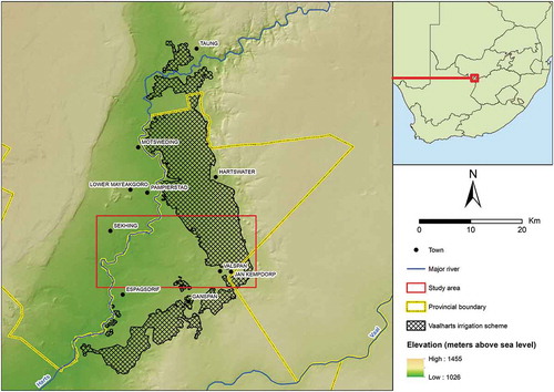
The study area (Figure 1) is located in the Vaalharts irrigation scheme in the Northern Cape Province of South Africa. The irrigation scheme is situated at the confluence of the Harts and Vaal Rivers and has a scheduled area of 291.81 km² (Van Vuuren 2010). The region has a steppe climate with an average annual temperature of 18.6°C and an average annual rainfall of 437 mm. The selected study site is 303.12 km² in size and contains a variety of land covers, including indigenous vegetation, built up, bare ground, water and crops. Cotton, maize, wheat, barley, lucerne, groundnuts, canola and pecan nuts are all grown in the area on a crop rotation basis (Nel and Lamprecht 2011; Muller and Van Niekerk 2016).

Figure 1. Study area Vaalharts irrigation scheme (380 km²), Northern Cape, South Africa

2.2 Data acquisition and pre-processing

Three remote sensing datasets were used in this study, namely LiDAR data, aerial photographs and satellite imagery (Figure 2).

Figure 2. Raw aerial imagery (a), Sentinel-2 (b), LiDAR intensity (c) and LiDAR nDSM (d)

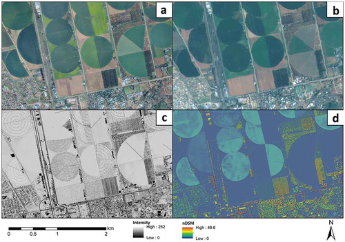
The LiDAR data and aerial imagery were collected by Land Resources International for the Northern Cape Department of Agriculture, Land Reform and Rural Development. The data were acquired between 19 and 29 February 2016 with a Leica ALS50-II LiDAR sensor at an altitude of 4500 ft. The LiDAR data have an average point spacing of 0.7 m and an average point density of 2.04 m². The aerial imagery was acquired between 22 February and 18 March 2016 with a PhaseOne iXA sensor at an altitude of 7500 ft. The imagery consisted of four bands, namely blue, green, red and Near-Infrared (NIR) with the RGB bands having a Ground Sampling Distance (GSD) of 0.1 m and the NIR a GSD of 0.5 m. The RGB bands of the aerial images were resampled to 0.5 m to match the resolution of the NIR band. This dataset was labeled A2. The analysis was also performed on the aerial imagery (A1) at its original resolution (0.1 m for the red, green and blue bands and 0.5 m for the NIR band) in order to assess whether down sampling makes any statistically significant difference. The spectral information of the aerial imagery is shown in Table 1.

Table 1. Spectral information for the aerial imagery

Bands	Wavelength (nm)	Resolution (m)
Blue	450–480	0.1
Green	550–580	0.1
Red	650–680	0.1
NIR	720–2500	0.5

The Sentinel-2 image was acquired on 10 February 2016. This image was selected because it was the closest cloud-free temporal match to the LiDAR data and aerial photography. Ten bands were used for analysis as shown in Table 2. The Sentinel-2 image was atmospherically corrected using ATCOR in PCI Geomatica 2018. Since the Sentinel-2 image was acquired at level-1 C orthorectification was already performed on the imagery and thus not required.

Table 2. Sentinel-2 bands used for analysis

Bands	Central wavelength (µm)	Resolution (m)	Bandwidth (nm)
Band 2 – Blue	0.490	10	65
Band 3 – Green	0.560	10	35
Band 4 – Red	0.665	10	30
Band 5 – Vegetation red edge	0.705	20	15
Band 6 – Vegetation red edge	0.740	20	15
Band 7 – Vegetation red edge	0.783	20	20
Band 8 – NIR	0.842	10	115
Band 8A – Narrow NIR	0.865	20	20
Band 11 – SWIR	1.610	20	90
Band 12 – SWIR	2.190	20	180

Four features were derived from the LiDAR data, namely an nDSM, generalized nDSM (gen-nDSM), an intensity image and a multi-return value raster. The nDSM was created by interpolating a 2 m resolution DSM and DTM and subtracting the DTM from the DSM. Inverse Distance Weighted (IDW) interpolation was used for the interpolations. A generalized DSM (gen-nDSM) was created by calculating the range of values within a 5 × 5 moving window. A 5 × 5 window was chosen in order to keep the effective resolution below 10 m. This range was also suggested by Mathews and Jensen (2012), who found that nDSM range within a small window is useful for differentiating between low and high vegetation. The intensity image was interpolated at a resolution of 2 m using IDW. The nDSM, gen-nDSM, and intensity image were created using ArcGIS 10.4. A 10 m resolution multi-return value raster was created by using LiDAR360 1.3. PCI Geomatica was used to apply Histogram-Based Texture Measures (HISTEX) and Texture Analysis (TEX) on the nDSM and intensity image, using a 5 × 5 window size. Highly correlated texture features were excluded. The LiDAR derivatives were interpolated/created to match the spatial resolution of the Sentinel-2 bands (2, 3, 4 and 8), which had a resolution of 10 m. The image texture was incorporated in accordance with Liu and Yanchen (2015). The LiDAR-based features considered in this study are listed in Table 3.

Table 3. LiDAR features used as input to the classifiers

Type	Features	Number of features
LiDAR Derivatives	nDSM	4
	Intensity
	Focal nDSM
	Multi returns
Textural features	HISTEX: mean, median, mean deviation from mean, mean deviation from median, entropy, weighted-rank fill ratio	12
	TEX: homogeneity, contrast, dissimilarity, mean, variance, entropy, angular second moment, correlation, inverse difference	18
	Total number of features:	34

A Principle Component Analysis (PCA) was performed on the aerial imagery bands. The same texture features that were used for the LiDAR data were applied to the first principal component (PC1). To accommodate the higher resolution of the aerial imagery, a 51 × 51 window size was used for generating the texture features from the A1 dataset. The 51 × 51 window size was selected to match the LiDAR texture resolution, resulting in an effective resolution of 5.1 m. The features generated from the aerial imagery are listed in Table 4. Due to the lower resolution of the A2 dataset, texture feature were not generated for the A2 dataset.

Table 4. Aerial features used as input to the classifiers

Type	Features	Number of features
Spectral bands	Blue	4
	Green
	Red
	NIR
Textural features	HISTEX: mean, median, mean deviation from mean, mean deviation from median, entropy, weighted-rank fill ratio	6
	TEX: homogeneity, contrast, dissimilarity, mean, variance, entropy, angular second moment, correlation, inverse difference	9
	Total number of features:	19

The features stemming from the Sentinel-2 imagery are the 10 bands that had resolutions equal or higher than 20 m (Table 2).

By using three data sources (LiDAR, aerial, and satellite data) individually and in combination, seven different experiments were created, namely aerial (A2 and A1), LiDAR (L), Sentinel-2 (S), aerial and Sentinel-2 (A-S), aerial and LiDAR (A-L), LiDAR and Sentinel-2 (L-S), and lastly LiDAR, aerial and Sentinel-2 (A-S-L). Table 5 lists the eight input datasets considered.

Table 5. Summary of the different experiments of datasets

ID	Dataset	Number of features
A1	Aerial	14
A2	Aerial	19
S	Sentinel-2	10
L	LiDAR	34
A-S	Aerial (A2) & Sentinel-2	23
A-L	Aerial (A2) & LiDAR	47
L-S	LIDAR & Sentinel-2	44
A-S-L	Aerial (A2), Sentinel-2 and LiDAR	57

Note: The first column shows the unique identifier; the characters represent the data contained in the dataset, with A indicating aerial imagery, S indicating Sentinel-2 imagery, and L indicating LiDAR data.

The datasets were standardized using zero-mean and unit variance standardization (Jonsson et al. 2002), which can be expressed as

$x^{\prime }=\frac{x-\bar{x}}{\sigma }$

Where x is the original value, $\bar{x}$ is the mean of the feature and σ is the standard deviation of the feature.

2.3 Reference data

A vector database containing crop type data was obtained from GWK (www.gwk.co.za), an agribusiness operating in the study area. The database contains polygons for three crop types, namely, maize, cotton and groundnuts. A fourth crop type, orchard, was added to the database by visual image interpretation and manual digitizing from aerial imagery. Stratified random sampling was used to create 1000 data points from the crop type database. Each target class (maize, cotton, groundnuts, orchard, and non-agriculture) was allocated 200 random sample points.

2.4 Classification and accuracy assessment

The classifications were performed using the Scikit-learn 0.18.2 python library. Scikit-learn is an open-source machine learning library developed by Pedregosa et al. (2012) and includes a wide range of classification algorithms and metrics, including OA and Kappa (K). The Tensorflow 1.2.1 library (Abadi et al. 2016) was used to perform a d-NN classification, while XGBoost 0.7 (T. Chen et al. 2017) was used to perform the XGBoost classification. The d-NN classifier was set to three hidden layers and the other classifiers were configured to use the default parameters.

The algorithms were iterated a hundred times in order to cross-validate and assess the stability of the models. For each iteration, the reference dataset was randomly split into a training (70% of samples) and accuracy assessment (30% of samples) subset. Classification algorithm performance was assessed using four metrics, namely, OA, K, f-score, and Standard Deviation (SD) of OA. The latter metric was used to assess model stability. The thematic crop type maps resulting from the classifications were also qualitatively assessed by means of visual comparisons.

The Friedman test (Zimmerman and Zumbo 1993) was used to compare the results from the different classifiers and experiments. The Friedman test is a non-parametric alternative to a repeated-measure ANOVA and can be used with ordinal, interval and ratio data (Zimmerman and Zumbo 1993; Sheldon, Fillyaw, and Thompson 1996). P-values lower than 0.05 were considered significant.

3. Results

The results are summarized in Table 6. For sake of readability, only the OAs are shown. Other metrics (Kappa, f-score and standard deviation of the OA) are provided in the Appendix A.

Table 6. Overall accuracy results for the seven datasets and the ten different classifiers

Classifier		Dataset
	A1	A2	S	L	A-S	A-L	L-S	A-S-L	Mean	Stdev
d-NN	81	55.2	90.8	83.2	92.3	88.2	91.5	92.2	84.3	11.7
DT	72.2	46.1	81	82.3	86.2	84.7	90.2	90	79.1	13.6
k-NN	77.1	54.5	85.8	83.9	88.9	87.7	91.2	92.1	82.7	11.5
LR	73.2	44.5	85.3	84.9	91.6	86.8	92.2	92.9	81.4	15.2
NB	62.5	46.7	67.9	77.7	74.8	81.2	84.7	86	72.7	12.4
NN	81.2	56.5	88.2	86.3	92.7	89.8	92.8	93.4	85.1	11.5
RF	81.9	54.4	86.5	87.3	93.1	90.7	93.2	94.6	85.2	12.3
SVM-L	73.4	44	88.3	86.2	92.6	88.2	93.5	93.5	82.5	15.8
SVM RBF	72	50.5	75.9	83.4	87	86.6	89.8	90.1	79.4	12.5
XGBoost	81.3	56.1	86.3	87.8	91.9	91.3	93	94.1	85.2	11.7
Mean	75.6	50.9	83.6	84.3	89.1	87.5	91.2	91.9
Stdev	5.8	4.8	6.6	2.8	5.3	2.8	2.5	2.4

3.1 Individual dataset–classifier combinations

The most accurate individual classification (OA of 94.6%) was achieved when the A-S-L (aerial, Sentinel-2 and LiDAR) dataset was used as input to the RF classifier (A-S-L> RF scenario). This was followed by the combination of XGBoost with A-S-L (OA of 94.1%); SVM-L with A-S-L (OA of 93.5%); SVM-L with L-S (OA of 93.5%); NN with A-S-L (OA of 93.4%); RF with L-S (OA of 93.2%); and RF with A-S (OA of 93.1%). Although there were no significant differences among the accuracies of the top three results (p > 0.05), the difference between the A-S-L> RF and L-S> SVM-L scenarios was significant (p = 0.022).

3.2 Dataset performance

Overall, the A-S-L and L-S datasets produced the highest mean OAs, with 91.9% and 91.2% respectively (see last two rows in Table 6). The A-S was the third best performing dataset with a mean OA of 89.1%. The mean OA of the A-S dataset was significantly lower than those of the A-S-L (p = 0.011) and L-S (p = 0.011) datasets, while the difference between A-S-L and L-S were not significant (p = 0.002). On average, the A2 dataset performed the worst with a mean OA of 50.9%. The A-S-L dataset obtained the lowest OA standard deviation values (2.4%) and all the datasets containing LiDAR data (L, A-L, L-S, A-S-L) obtained OA standard deviation values of 2.8% or lower. The datasets containing aerial data obtained OA standard deviation values between 4.8 and 5.8 and the S dataset obtained the highest OA standard deviation value of 6.6.

3.3 Classifier performance

Overall, RF (85.2%), XGboost (85.2%), NN (85.1%), and d-NN (84.3%) were the best performing classification algorithms (see last two columns in Table 6). The differences in mean OA of these classifiers were statistically insignificant (p = 0.119), which suggests that they performed on par with one another. When all five best performing classification algorithms (RF, XGboost, NN, d-NN and LR) were compared, the differences in mean OA were statistically significant (p = 0.001). Similarly, when all the classification algorithms were compared the difference in mean OA were statistically significant (p = 0). The standard deviations of OAs for the classifiers is high (11–16%), mainly due to the A2 dataset’s poor classification results. When the A2 dataset is omitted, the standard deviations drop sharply (4–9%), with RF, NN, XGboost, d-NN and k-NN having standard deviation values of 4–5%. This suggests that RF, NN, XGboost, d-NN and k-NN performed more consistently among different datasets compared to the other classification algorithms.

RF and XGBoost were the best performing classifiers, but d-NN and NN also performed well. NN and d-NN obtained higher OAs when used to classify the Sentinel-2 data, while RF and XGBoost obtained higher OAs when used to classify the LiDAR data. When the LiDAR and Sentinel-2 data were combined, RF and XGBoost classifiers obtained similar OAs, with the former outperforming the latter by only 0.2%. Furthermore, nine classifiers obtained their best OAs when performed on the aerial imagery, LiDAR and Sentinel-2 experiment (A-S-L), with only DT obtaining its highest OA for L-S. Eight of the classifiers (RF, XGBoost, DTs, k-NN, LR, d-NN, SVM-L and NN) obtained OAs higher than 90% when performed on the L-S experiment, whereas SVM RBF and NB obtained OAs of 84.7% and 89.8% respectively.

The following sections focus on the classification accuracies per crop type. For the sake of brevity, only the results of the best-performing classifier, RF, are shown.

3.4 RF per-class performance (per dataset)

A confusion matrix for each of the RF experiments is provided in the Appendix B. Table 6 summarizes the per-class performances of all experiments, while the errors of commission and omission are listed in Table 7.

Table 7. Error of commission and omission for all five class. Only the errors of commission and omission for the random forest classifier are shown

Class	Error (%)	A1	S	L	A-S	A-L	L-S	A-S-L
Non-Agri	Commission	21.8	8.3	23.2	5.8	17.2	8.8	5.8
	Omission	22.0	13.0	27.7	10.1	18.9	10.6	10.0
Maize	Commission	17.4	8.3	6.7	7.4	6.3	6.0	5.3
	Omission	19.4	2.4	3.1	1.0	2.2	1.5	1.5
Orchard	Commission	4.8	9.4	4.3	4.0	3.3	3.5	3.1
	Omission	12.3	21.2	6.2	6.4	6.5	3.9	3.7
Groundnut	Commission	23.7	19.8	16.1	7.8	10.7	6.8	5.1
	Omission	21.3	14.3	17.4	9.9	12.4	8.4	6.0
Cotton	Commission	23.1	21.6	13.6	9.8	8.8	8.9	7.6
	Omission	16.2	15.2	8.2	6.8	6.0	9.2	5.6

The A-S-L> RF experiment performed the best and was the only scenario in which the omission and commission errors were equal to or below 11% for all five classes. Generally, the non-agri class was the most confused with other classes. For instance, the non-agri class was most frequently misclassified as orchards, with the highest number (160) of false positives (FP) followed by groundnuts (108). Cotton and maize obtained low FP values of 47 and 26 respectively.

Similar to the A-S-L> RF experiment, the non-agri class was the most confused with other classes when the L-S dataset was used as input to the RF classifier. The errors of commission and omission of 8.8% and 10.6% respectively are also comparable to those obtained with the A-S-L> RF experiment.

The A-L> RF experiment performed relatively poorly, with the highest OA being 91.3% (XGBoost). Maize, orchard, and cotton performed on par with one another with and all three obtaining errors of commission and omission below 9%. Groundnuts was the second-worst performing crop type, with error of commission and omission values of 10.7% and 12.4% respectively. Non-agri was the worst performing class for the A-L> RF experiment with error of commission and omission values of 17.2% and 18.9% respectively.

In the L> RF experiment, maize, orchard and cotton were the most accurately classified, with errors of commission and omission below 10%, except for cotton which obtained an error of commission of 13.6%. Groundnuts obtained the highest error of commission (16.1%) and omission (17.4%) out of the crop classes. As with previous experiments, the non-agri was the most difficult to classify in this experiment, with error of commission and omission values of 23.2% and 27.7% respectively.

Out of all the single-sensor experiments, the S> RF experiment returned the lowest error of commission and omission values for the non-agri class. The non-agri class was the second-best performing class, with maize being the most successfully classified. Groundnuts and cotton performed on par with each other, but where the most difficult crop types to differentiate in the S> RF experiment.

Overall, A2> RF was the worst performing experiment, with orchard being the class that was most accurately classified. Maize was the second-best performing class for the A2> RF experiment, followed by non-agri and cotton (both obtained similar results). Groundnuts was the worst performing class. When the A2 dataset was used as input to RF, maize was most frequently confused with cotton, while non-agri and groundnuts were also often confused.

3.5 Qualitative evaluation

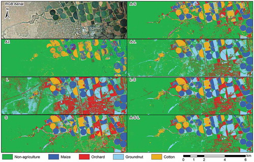
Figure 3 shows a visual comparison of seven experiments (A2> RF, S> RF, L> RF, A-S> RF, A-L> RF, L-S> RF and A-S-L> RF) and an RGB image for orientation. The main purpose of this qualitative evaluation is to compare the quantitative results to the spatially represented classified data. From visual inspection, the RF maps compare well with local knowledge. The only exception is in the A> RF experiment, in which non-agri was relatively well differentiated, while the majority of the fields were classified as either maize or cotton, which is not realistic. The L> RF experiment often misclassified non-agri as orchard and groundnuts. Natural vegetation, power lines and urban areas were most often confused with these classes. As shown in the confusion matrices, the S> RF experiment had the lowest number of misclassifications for non-agri, which seems to be in good agreement with the thematic map produced from the experiment. Based on a visual inspection, the L> RF experiment seems to have generated the most misclassifications. A comparison of the thematic maps produced by the S> RF and the L> RF experiments reveals that the former classified non-agri best. Conversely, the L> RF experiment classified crops better (more evenly). Combining the L and S datasets improved the crop type classifications, which is in agreement with the quantitative assessments (error of commission and omission values of below 11%). The A-S> RF and S> RF maps seem very similar, although the orchard class seems to be better depicted in the latter experiment. There is little difference between the A-L> RF, L-S> RF and A-S-L> RF maps, apart from in the non-agri class which seems to be better classified in the latter experiment, which corresponds with the quantitative assessments.

Figure 3. Visual comparison of the random forest classification algorithm for the seven experiments, with the RGB aerial photograph in the top left corner for orientation

4. Discussion

The experiments showed that five classes (non-agri, groundnuts, cotton, maize and orchards) can be accurately classified using machine learning and different combinations of data (aerial, LiDAR and Sentinel-2 data). Nine of the ten machine learning classification algorithms were able to obtain OA above 90%, with RF obtaining the highest OA (94.6%). The datasets used in this study were able to obtain acceptable OAs when used on their own as input for the machine learning algorithms, with LiDAR and Sentinel-2 obtaining similar OAs. However, when the datasets were combined, specifically the LiDAR and Sentinel-2 data, higher OAs were obtained.

Using only Sentinel-2 data (S> RF experiment) or aerial imagery (A1> RF and A2> RF experiments) as input to the RF classifier resulted in relatively high misclassifications among the orchard, groundnuts, maize and cotton classes. Groundnuts were mostly misclassified as cotton or orchard in the S> RF experiment, which was likely due to the similar spectral signatures of these classes (Figure 4). However, maize was the least misclassified in this experiment, obtaining low errors of commission (0.08%) and omission (0.02%) compared the other classes, despite having a spectral signature similar to cotton and groundnuts. These low errors were mainly due to maize being misclassified as non agri only 84 times, while other classes were misclassified as non agri at least 4 times more frequently. For the A1> RF experiment, groundnuts, non-agri, maize and cotton were frequently confused, while the orchard class was the most accurately classified (error of commission of 4.8% and error of omission of 12.3%). The relatively good performance of the VHR aerial imagery for mapping orchards was attributed to the ability of the texture features to represent the structural (spatial) characteristics of this class. Tree crops (mostly pecan nuts and fruit trees in the study area) are usually planted in rows and about 5–10 m apart. These rows are clearly visible in the VHR aerial imagery. In contrast, the resolution of the Sentinel-2 imagery is too low (10 m) to adequately represent the row structure of the orchards. This finding is in agreement with Warner and Steinmaus (2005) who achieved a UA of 97.3% and a PA of 88.7% when classifying orchard using VHR imagery.

Figure 4. Spectral responses of the five classes based on the Sentinel-2 bands considered

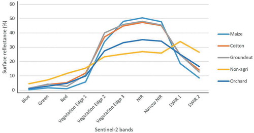
The non-agricultural (non-agri) class is much more heterogeneous than the other classes and as such is expected to have some spectral and structural overlap with the crop type classes. This explains why the non-agri class was often misclassified. Nevertheless, the Sentinel-2 data performed relatively well and even outperformed several of the other datasets that included additional features (e.g. texture measures), indicating the potential of Sentinel-2 data for crop type classification. This agrees with Vuolo et al. (2018), who obtained OAs of above 90% when using Sentinel-2 imagery for crop type classification. Similarly, Belgiu and Csillik (2018) created crop type maps using Sentinel-2 data in three test areas and obtained OAs ranging from 75% to 98%.

Groundnuts obtained the highest error of commission and omission in the A2> RF experiment, which was unexpected due to groundnuts being planted in rows, which would have been best represented by the texture features. However, groundnuts are planted with row spacings of 45 cm up to 76 cm, which is likely too narrow to be adequately depicted by the resolution of the aerial imagery. Similarly, the maize and cotton crop classes did not benefit from the texture feature as they are planted in too narrow rows.

The LiDAR data (L dataset) performed well on its own, despite not having the benefit of spectral information. However, it only performed well when there were substantial height differences between the target crops (e.g. between orchards and groundnuts). Based on the visual and quantitative analyses it is clear that most misclassifications involving the LiDAR data could be attributed to within-field height variations (canopy gaps or areas with poor crop growth), which causes tall crops (orchards) to have similar height values to short crops such as groundnuts (around zero height) and intermediately tall crops such as maize and cotton (0–2 m). Heights of cotton and maize varied substantially within and among fields across the study area, which resulted in many areas within maize fields as having the same height as cotton. These variations in heights could explain why there were misclassifications between cotton and maize for the L experiment. For the same reason, the non-agri class was the most confused when the LiDAR data was used on its own as it contains land covers (natural vegetation, trees, man-made structures) that have similar heights to many of the crop type classes considered. For instance, because it has a height of close to zero in the LiDAR data, groundnuts were most frequently misclassified as short vegetation and bare areas within the non-agri class. This observation is in agreement with Mathews and Jensen (2012), who found that non-agri and other crops are often confused for vineyards when only LiDAR data are used as classifier input.

The L-S dataset, which is the combination of the L and S datasets, seemed have to retained the benefits of the two data sources (high OA of 93.5% using the SVM-L classifier). The addition of the L dataset to the S dataset helped to minimize misclassifications among the four crop types (resulting in errors of commission and omission of below 10.6%). A mean OA increase of 7.1% when the LiDAR data were added to the Sentinel-2 image corresponds with other studies (Antonarakis, Richards, and Brasington 2008; Chen et al. 2009; Jahan and Awrangjeb 2017; Liu and Yanchen 2015; Matikainen et al. 2017; Wu et al. 2017) where substantially higher OAs were obtained when LiDAR data were added to spectral data. Similar improvements in accuracy were observed in the A-L experiment, which corresponds well with Chen et al. (2009).

The Sentinel-2 imagery performed the best of all the single-source datasets considered. Although the LiDAR data performed on par with the Sentinel-2 imagery for crop type differentiation, the latter data have the advantage of being regularly updated (once every five days, depending on cloud cover), while LiDAR data are typically updated less frequently (once every few years when obtained using aircraft). LiDAR data are also relatively expensive to collect, whereas Sentinel-2 data can be obtained freely. Vuolo et al. (2018) showed that crop type classification accuracies increased when multiple Sentinel-2 images, collected over a growing season, were used as input to machine learning classifiers. Consequently, the value of using LiDAR data in combination with multi-temporal Sentinel-2 data may be worth investigating in future work.

The availability of LiDAR data is likely to increase as satellite-based systems become operational and as LiDAR sensors mounted on UAVs become more common. However, LiDAR data are only recommended for crop type classification if the crop types being classified have sufficient height differences. It is clear from our findings that, if it is available, LiDAR data should be combined with spectral data to improve classifications, especially for differentiating crop types that have similar spectral properties, but are also structurally different (i.e. have different heights).

The aerial imagery (A1 and A2) did not perform as well as the Sentinel and LiDAR datasets. This can be partly attributed to the aerial imagery’s lower spectral resolution of four bands (blue, green, red and near-infrared) compared to the Sentinel-2 imagery, but the main contributing factor to the poor performance of the aerial imagery is its high spatial resolution. At 0.5 m resolution the imagery represented individual plants/trees and inter-row bare ground and cover crops. This additional information likely caused large spectral variations (noise) within fields, which the per-pixel machine learning algorithms were not able to handle (i.e. each field represented multiple land covers). This inference is supported by the improvement in performance noted when texture measures were added as predictor variables (A1), which effectively converted the spectral variations into useful information. Based on our results, the use of such data for crop type classification is not recommended, especially given that Sentinel-2 data generally performed better and are readily (and more frequently) available.

Although the main focus of the study was not to compare the accuracies of different classification algorithms, we can recommend RF or XGBoost when only LiDAR data is available, while the d-NN or SVM-L algorithms are most suitable for when Sentinel-2 imagery is the only available data source. When using a combination of LiDAR and Sentinel-2 data, either XGBoost, RF, d-NN or SVM-L performed well with our data.

5. Conclusion

To our knowledge, this is the first study in which LiDAR data was used on its own as input to machine learning algorithms for differentiating multiple crop types. Experiments involving combinations of aerial, Sentinel-2 and LiDAR data were carried out to assess the impact of combining the different data sources on classification accuracies. It was shown that most crops could be differentiated with LiDAR data on its own, with XGBoost providing the best accuracies (87.8%). The LiDAR data proved particularly useful for differentiating crops with substantial height differences (e.g. orchards from groundnuts). In general, the classifications in which LiDAR derivatives were used as the only predictor variables were comparable with those in which Sentinel-2 data were used on its own. However, it is clear from the results that the machine learning classifiers were most effective when the different data sources were combined, with the combination of all three sources (i.e. aerial imagery, LiDAR and Sentinel-2 data) providing the highest accuracies (94.6% when RF was used as classifier). Using the aerial imagery on its own produced the lowest accuracies (mean OA of 75.6%).

The findings of this research can aid in solving the real-world problem of monitoring crop production, since this research has provided valuable information on crop type classification. The research provided useful information on which sources of remotely sensed data are most effective for crop type classification, either on its own or in combination. It also showed which machine learning algorithms are most effective and robust for differentiating a range of crop types. This provides of a foundation for selecting the appropriate combination of remotely sensed data sources and machine learning algorithms for operational crop type mapping.

Additional information

Funding

This work forms part of a larger project titled “Salt Accumulation and Waterlogging Monitoring System (SAWMS) Development” which was initiated and funded by the Water Research Commission (WRC) of South Africa (contract number K5/2558//4). More information about this project is available in WRC Report No TT 782/18, titled SALT ACCUMULATION AND WATERLOGGING MONITORING SYSTEM (SAWMS) DEVELOPMENT (ISBN 978-0-6392-0084-2) available at www.wrc.org.za. This work was also supported by the National Research Foundation (grant number 112300). The authors would also like to thank www.linguafix.net for their language editing services.

Notes on contributors

Adriaan Jacobus Prins

Adriaan Jacobus Prins received his Msc degree from Stellenbosch University in 2019. His research interests are in the application of remote sensing data (LiDAR, very high-resolution imagery or satellite imagery) along with machine learning techniques to develop geographical information systems (GIS) products.

Adriaan Van Niekerk

Adriaan Van Niekerk (PhD Stellenbosch University) is the Director of the Centre for Geographical Analysis (CGA) and Professor at Stellenbosch University. His research interests are in the application and development of geographical information systems (GIS) and remote sensing (earth observation) techniques to support decisions concerned with land use, bio-geographical, environmental and socio-economic problems.

References

- Abadi, M., P. Barham, J. Chen, Z. Chen, A. Davis, J. Dean, M. Devin, et al. 2016. “TensorFlow: A System for Large-Scale Machine Learning.” 12th USENIX Symposium on Operating Systems Design and Implementation (OSDI ’16), Savannah, GA, 265–284.
- Al-doski, J., S. B. Mansor, H. Zulhaidi, and M. Shafri. 2013. “Image Classification in Remote Sensing.” Journal of Environment and Earth Science 3 (10): 141–147.
- Antonarakis, A. S., K. S. Richards, and J. Brasington. 2008. “Object-Based Land Cover Classification Using Airborne LiDAR.” Remote Sensing of Environment 112 (6): 2988–2998. doi:10.1016/j.rse.2008.02.004.
- Belgiu, M., and O. Csillik. 2018. “Sentinel-2 Cropland Mapping Using Pixel-Based and Object-Based Time-Weighted Dynamic Time Warping Analysis.” Remote Sensing of Environment 204 (January 2017): 509–523. doi:10.1016/j.rse.2017.10.005.
- Brennan, R., and T. L. Webster. 2006. “Object-Oriented Land Cover Classification of Lidar-Derived Surfaces.” Canadian Journal of Remote Sensing 32 (2): 162–172. doi:10.5589/m06-015.
- Campbell, J. B., and R. H. Wynne. 2011. Introduction to Remote Sensing. Uma Ética Para Quantos? Fifth Edit. Vol. XXXIII. New York: Guilford Press.
- Charaniya, A. P., R. Manduchi, and S. K. Lodha. 2004. “Supervised Parametric Classification of Aerial LiDAR Data.” IEEE Computer Society Conference on Computer Vision and Pattern Recognition Workshops, Washington, DC, 30.
- Chen, T., H. Tong, M. Benesty, V. Khotilovich, and Y. Tang. 2017. “Package Xgboost - R Implementation.”.
- Chen, Y., W Su, J Li, and Z. Sun. 2009. “Hierarchical Object Oriented Classification Using Very High Resolution Imagery and LIDAR Data over Urban Areas.” Advances in Space Research 43 (7): 1101–1110. doi:10.1016/j.asr.2008.11.008.
- Chica-Olmo, M., and F. Abarca-Hernández. 2000. “Computing Geostatistical Image Texture for Remotely Sensed Data Classification.” Computers & Geosciences 26 (4): 373–383. doi:10.1016/S0098-3004(99)00118-1.
- Dell’Acqua, F., G. C. Iannelli, M. A. Torres, and M. L. V. Martina. 2018. “A Novel Strategy for Very-Large-Scale Cash-Crop Mapping in the Context of Weather-Related Risk Assessment, Combining Global Satellite Multispectral Datasets, Environmental Constraints, and in Situ Acquisition of Geospatial Data.” Sensors (Switzerland) 18 (2): 2. doi:10.3390/s18020591.
- Escobar, V., and M. Brown. 2014. “ICESat--2 Applications Vegetation Tutorial with Landsat 8 Report.” http://icesat.gsfc.nasa.gov/icesat2/applications/ICESat2_Vegetation_Report_FINAL.pdf
- Estrada, J., H. Sánchez, L. Hernanz, M. Checa, and D. Roman. 2017. “Enabling the Use of Sentinel-2 and LiDAR Data for Common Agriculture Policy Funds Assignment.” ISPRS International Journal of Geo-Information 6 (8): 255. doi:10.3390/ijgi6080255.
- Gilbertson, J. K., J. Kemp, and Adriaan Van Niekerk. 2017. “Effect of Pan-Sharpening Multi-Temporal Landsat 8 Imagery for Crop Type Differentiation Using Different Classification Techniques.” Computers and Electronics in Agriculture 134: 151–159. doi:10.1016/j.compag.2016.12.006.
- Immitzer, M., F. Vuolo, and C. Atzberger. 2016. “First Experience with Sentinel-2 Data for Crop and Tree Species Classifications in Central Europe.” Remote Sensing 8 (3): 3. doi:10.3390/rs8030166.
- Inglada, J., M. Arias, B. Tardy, O. Hagolle, S. Valero, D. Morin, G. Dedieu et al. 2015. “Assessment of an Operational System for Crop Type Map Production Using High Temporal and Spatial Resolution Satellite Optical Imagery.” Remote Sensing 7 (9): 12356–12379. DOI:10.3390/rs70912356.
- Ismail, Z., M. F. Abdul Khanan, F. Z. Omar, M. Z. Abdul Rahman, and M. R. Mohd Salleh. 2016. “Evaluating Error Of Lidar Derived Dem Interpolation For Vegetation Area” XLII (October): 3–5.
- Jahan, F., and M. Awrangjeb. 2017. “Pixel-Based Land Cover Classification by Fusing Hyperspectral and LiDAR Data.” International Archives of the Photogrammetry, Remote Sensing and Spatial Information Sciences - ISPRS Archives 42 (2W7): 711–718. doi:10.5194/isprs-archives-XLII-2-W7-711-2017.
- Jonsson, K., J. Kittler, Y. P. Li, and J. Matas. 2002. “Support Vector Machines for Face Authentication.” Image and Vision Computing 20 (4): 369–375. doi:10.1016/S0262-8856(02)00009-4.
- Lary, D. J., A. H. Alavi, A. H. Gandomi, and A. L. Walker. 2016. “Machine Learning in Geosciences and Remote Sensing.” Geoscience Frontiers 7 (1): 3–10. doi:10.1016/j.gsf.2015.07.003.
- Liaqat, M. U., M. J. Masud Cheema, W. Huang, T. Mahmood, M. Zaman, and M. M. Khan. 2017. “Evaluation of MODIS and Landsat Multiband Vegetation Indices Used for Wheat Yield Estimation in Irrigated Indus Basin.” Computers and Electronics in Agriculture 138: 39–47. doi:10.1016/j.compag.2017.04.006.
- Liu, X., and B. Yanchen. 2015. “Object-Based Crop Species Classification Based on the Combination of Airborne Hyperspectral Images and LiDAR Data.” Remote Sensing 7 (1): 922–950. doi:10.3390/rs70100922.
- Matese A., P. Toscano, S. Filippo Di Gennaro, L. Genesio, F. P. Vaccari, J. Primicerio, C. Belli, A. Zaldei, R. Bianconi, and B. Gioli. 2015. “Intercomparison of UAV, Aircraft and Satellite Remote Sensing Platforms for Precision Viticulture.” Remote Sensing 7 (3): 2971–2990. doi:10.3390/rs70302971.
- Mathews, A. J., and J. L. R. Jensen. 2012. “An Airborne LiDAR-Based Methodology for Vineyard Parcel Detection and Delineation.” International Journal of Remote Sensing 33 (16): 5251–5267. doi:10.1080/01431161.2012.663114.
- Matikainen, L., K. Karila, J. Hyyppä, P. Litkey, E. Puttonen, and E. Ahokas. 2017. “Object-Based Analysis of Multispectral Airborne Laser Scanner Data for Land Cover Classification and Map Updating.” ISPRS Journal of Photogrammetry and Remote Sensing 128: 298–313. doi:10.1016/j.isprsjprs.2017.04.005.
- Matton, N., G. S. Canto, F. Waldner, S. Valero, D. Morin, J. Inglada, M. Arias, S. Bontemps, B. Koetz, and P. Defourny. 2015. “An Automated Method for Annual Cropland Mapping along the Season for Various Globally-Distributed Agrosystems Using High Spatial and Temporal Resolution Time Series.” Remote Sensing 7 (10): 13208–13232. doi:10.3390/rs71013208.
- Mattupalli, C., C. Moffet, K. Shah, and C. Young. 2018. “Supervised Classification of RGB Aerial Imagery to Evaluate the Impact of a Root Rot Disease.” Remote Sensing 10 (6): 917. doi:10.3390/rs10060917.
- Muller, S. J., and Adriaan Van Niekerk. 2016. “International Journal of Applied Earth Observation and Geoinformation an Evaluation of Supervised Classifiers for Indirectly Detecting Salt-Affected Areas at Irrigation Scheme Level.” International Journal of Applied Earth Observations and Geoinformation 49: 138–150. doi:10.1016/j.jag.2016.02.005.
- Nel, A. A., and S. C. Lamprecht. 2011. “Crop Rotational Effects on Irrigated Winter and Summer Grain Crops at Vaalharts.” South African Journal of Plant and Soil 28 (2): 127–133. doi:10.1080/02571862.2011.10640023.
- Pádua, L., T. Adão, J. J. Jonáš Hruška, E. P. Sousa, R. Morais, and A. Sousa. 2017. “Very High Resolution Aerial Data to Support Multi-Temporal Precision Agriculture Information Management.” Procedia Computer Science 121: 407–414. doi:10.1016/j.procs.2017.11.055.
- Pedregosa, F., G. Varoquaux, A. Gramfort, V. Michel, B. Thirion, O. Grisel, M. Blondel, et al. 2012. “Scikit-Learn: Machine Learning in Python.” Journal of Machine Learning Research 12: 2825–2830.
- Peña-Barragán, J. M., M. K. Ngugi, R. E. Plant, and J. Six. 2011. “Object-Based Crop Identification Using Multiple Vegetation Indices, Textural Features and Crop Phenology.” Remote Sensing of Environment 115 (6): 1301–1316. doi:10.1016/j.rse.2011.01.009.
- Prins, A. 2019. “Efficacy of Machine Learning and Lidar Data for Crop Type Mapping.” Masters Thesis. Stellenbosch University.
- Rajan, N., and S. J. Maas. 2009. “Mapping Crop Ground Cover Using Airborne Multispectral Digital Imagery.” Precision Agriculture 10 (4): 304–318. doi:10.1007/s11119-009-9116-2.
- Sankey, T., J. Donager, J. McVay, and J. B. Sankey. 2017. “UAV Lidar and Hyperspectral Fusion for Forest Monitoring in the Southwestern USA.” Remote Sensing of Environment 195: 30–43. doi:10.1016/j.rse.2017.04.007.
- Satale, D. M., and M. N. Kulkarni. 2003. “LiDAR in Mappingo.” Geospatial World. https://www.geospatialworld.net/article/lidar-in-mapping/
- Senthilnath, J., S. Kulkarni, J. A. Benediktsson, and X.-S. Yang. 2016. “A Novel Approach for Multi-Spectral Satellite Image Classification Based on the Bat Algorithm.” IEEE Geoscience and Remote Sensing Letters 13 (4): 599–603. doi:10.1109/LGRS.2016.2530724.
- Sheldon, M. R., M. J. Fillyaw, and W. D. Thompson. 1996. “The Use and Interpretation of the Friedman Test in the Analysis of Ordinal-Scale Data in Repeated Measures Designs.” Physiotherapy Research International: The Journal for Researchers and Clinicians in Physical Therapy 1 (4): 221–228. doi:10.1002/pri.66.
- Siachalou, S., G. Mallinis, and M. Tsakiri-Strati. 2015. “A Hidden Markov Models Approach for Crop Classification: Linking Crop Phenology to Time Series of Multi-Sensor Remote Sensing Data.” Remote Sensing 7 (4): 3633–3650. doi:10.3390/rs70403633.
- Turker, M., and A. Ozdarici. 2011. “Field-Based Crop Classification Using SPOT4, SPOT5, IKONOS and QuickBird Imagery for Agricultural Areas: A Comparison Study.” International Journal of Remote Sensing 32 (24): 9735–9768. doi:10.1080/01431161.2011.576710.
- Turker, M., and E. H. Kok. 2013. “Field-Based Sub-Boundary Extraction from Remote Sensing Imagery Using Perceptual Grouping.” ISPRS Journal of Photogrammetry and Remote Sensing 79: 106–121. doi:10.1016/j.isprsjprs.2013.02.009.
- Valero, S., D. Morin, J. Inglada, G. Sepulcre, M. Arias, O. Hagolle, G. Dedieu, S. Bontemps, P. Defourny, and B. Koetz. 2016. “Production of a Dynamic Cropland Mask by Processing Remote Sensing Image Series at High Temporal and Spatial Resolutions.” Remote Sensing 8 (1): 1–21. doi:10.3390/rs8010055.
- Vega, F. A., F. C. Ramírez, M. P. Saiz, and F. O. Rosúa. 2015. “Multi-Temporal Imaging Using an Unmanned Aerial Vehicle for Monitoring a Sunflower Crop.” Biosystems Engineering 132: 19–27. doi:10.1016/j.biosystemseng.2015.01.008.
- Vuolo, F., M. Neuwirth, M. Immitzer, C. Atzberger, and W. T. Ng. 2018. “How Much Does Multi-Temporal Sentinel-2 Data Improve Crop Type Classification?” International Journal of Applied Earth Observation and Geoinformation 72 (July): 122–130. doi:10.1016/j.jag.2018.06.007.
- Vuuren, L. V. 2010. “Vaalharts - A Garden in the Desert.” Water Wheel 9 (1): 20–24.
- Warner, T. A., and K. Steinmaus. 2005. “Spatial Classification of Orchards and Vineyards with High Spatial Resolution Panchromatic Imagery.” Photogrammetric Engineering and Remote Sensing 71 (2): 179–187. doi:10.14358/PERS.71.2.179.
- Wu, M., C. Yang, X. Song, W. C. Hoffmann, W. Huang, Z. Niu, C. Wang, and L. Wang. 2017. “Evaluation of Orthomosics and Digital Surface Models Derived from Aerial Imagery for Crop Type Mapping.” Remote Sensing 9 (3): 1–14. doi:10.3390/rs9030239.
- Yan, W. Y., A. Shaker, and N. El-Ashmawy. 2015. “Urban Land Cover Classification Using Airborne LiDAR Data: A Review.” Remote Sensing of Environment 158: 295–310. doi:10.1016/j.rse.2014.11.001.
- Yang, C., J. H. Everitt, D. Qian, B. Luo, and J. Chanussot. 2013. “Using High-Resolution Airborne and Satellite Imagery to Assess Crop Growth and Yield Variability for Precision Agriculture.” Proceedings of the IEEE 101 (3): 582–592. doi:10.1109/JPROC.2012.2196249.
- Zhang, R., and D. Zhu. 2011. “Study of Land Cover Classification Based on Knowledge Rules Using High-Resolution Remote Sensing Images.” Expert Systems with Applications 38 (4): 3647–3652. doi:10.1016/j.eswa.2010.09.019.
- Zi re 3,jhou, W. 2013. “An Object-Based Approach for Urban Land Cover Classification: Integrating LiDAR Height and Intensity Data.” IEEE Geoscience and Remote Sensing Letters 10 (4): 928–931. doi:10.1109/LGRS.2013.2251453.
- Zimmerman, D. W., and B. D. Zumbo. 1993. “Relative Power of the Wilcoxon the Friedman Test, and Repeated Test, Measures ANOVA on Ranks.” Journal of Experimental Education 62 (1): 75–86. doi:10.1080/00220973.1993.9943832.