Trajectory analysis at intersections for traffic rule identification

ABSTRACT

In this paper, we focus on trajectories at intersections regulated by various regulation types such as traffic lights, priority/yield signs, and right-of-way rules. We test some methods to detect and recognize movement patterns from GPS trajectories, in terms of their geometrical and spatio-temporal components. In particular, we first find out the main paths that vehicles follow at such locations. We then investigate the way that vehicles follow these geometric paths (how do they move along them). For these scopes, machine learning methods are used and the performance of some known methods for trajectory similarity measurement (DTW, Hausdorff, and Fréchet distance) and clustering (Affinity propagation and Agglomerative clustering) are compared based on clustering accuracy. Afterward, the movement behavior observed at six different intersections is analyzed by identifying certain movement patterns in the speed- and time-profiles of trajectories. We show that depending on the regulation type, different movement patterns are observed at intersections. This finding can be useful for intersection categorization according to traffic regulations. The practicality of automatically identifying traffic rules from GPS tracks is the enrichment of modern maps with additional navigation-related information (traffic signs, traffic lights, etc.).

KEYWORDS:

• Traffic rules
• traffic regulators
• GPS trajectories
• intersection classification
• speed-profiles
• clustering
• similarity measures

1. Introduction

With the development of mobile positioning devices and cloud computing technologies in recent years, collecting and processing mobile position information has become easier. The fact that modern databases can effectively store, process, and retrieve massive mobile positioning data has promoted the research on trajectory data mining (Zheng 2015). Through the analysis of trajectory data, it is possible to predict human activities (Makris and Ellis 2002, 2003; Hu, Xie, and Tan 2004; Piciarelli and Foresti 2005) and identify vehicles’ movement patterns (Gudmundsson, Laube, and Wolle 2008). For example, processing trajectory data from urban transportation can provide a good solution for optimized transportation routes, road condition prediction, and urban planning (Feng and Zhu 2016). Intersections are locations where two or more roads meet or cross, with the most common intersection types being the crossroads (4-way intersection) and T-intersections. Traffic rules regulate how traffic participants should cross those locations. Depending on intersection complexity and traffic flow, different traffic rules areset. At intersections with heavy traffic, most often there are traffic lights, while at locations with low traffic, there are traffic-signs that indicate the priority or yield of the vehicles from each direction (Åberg 1998). Other intersections may be uncontrolled, with no traffic lights or signs, where the right-of-way-rule is applicable. As hubs of urban roads, intersections restrict the traffic capacity of the entire area and for this reason, traffic congestion events and accidents are closely related to them (Solomon et al. 2006). Therefore, understanding and studying the traffic conditions at intersections can be beneficial for traffic planning.

This study is motivated by the need to find a way to extract movement patterns at intersection locations, by analyzing GPS tracks. In particular, given a set of trajectories, we want to find the different ways that vehicles move at those locations, that is 1) in which possible directions, and then 2) per direction, to find out the different ways they move along that direction. For example, from west to east, there might be two different ways to move along this given direction: without stopping and with a short stop. The final aim is to explore if the identified movement patterns at intersections can be indicative of the traffic regulation that applies at those locations. If so, traffic rules can be automatically identified by analyzing vehicles’ movement patterns from GPS trajectories, which means that, in practice, maps can be further enriched with intersection-related attributes such as traffic-rules. This kind of information is subject to changes – therefore, an approach that collects it in a potentially continuous fashion is highly relevant.

2. Related work

We identify two main thematic topics related to the aim of this study: 1) learning semantic scene models (activity modeling) and 2) traffic regulation detection and recognition from GPS tracks. Regarding the first topic, the aim of learning a semantic scene model is to derive the structure of a scene from trajectories obtained by tracking moving objects (pedestrians, vehicles, etc.). Given that the structure of a scene affects the motion of moving objects, by analyzing multiple observations from the scene, the structure of the scene can be revealed. The hypothesis here is that objects show similar motion preferences in space when crossing the same scene, that is pedestrians and vehicles do not move in a scene in an unstructured way or randomly.

Makris and Ellis (2003, 2005) were among the firsts to propose an activity-based semantic scene modeling method, where the model is learned through unsupervised learning and it is intended as a means for supporting the interpretation of the interaction of a target object with the scene. The entry/exit zones, routes, paths, and intersections are considered as semantic entities. Entry/exit zones are learned using two clustering algorithms: K-means and Expectation-Minimization (EM), with the latter outperforming the former. The found locations are represented with ellipses defined from Gaussian Models (GMs). Routes, paths, and intersections are derived hierarchically. First, the geometric model of the route is derived based on the separation distances between the trajectories. Processing proceeds in an on-line way, so in every comparison of a pair of trajectories, the position of route nodes is updated (or when necessary, new nodes are introduced in new positions). Paths are derived from routes according to merging criteria, and intersections are defined at the locations where routes diverge. The distribution of the route-learning set of trajectories is estimated over each geometric route model and the trajectories are then classified to routes using a Fuzzy Logic trajectory classifier. Low-Level Hidden Markov Models (LLHMM) are defined, with states representing the nodes of all route models, and temporal predictions of the state of an object being at time-step k + K, given the observation vector at time-step k is done under the HMM prediction framework (K denotes a future time-step). Atypical trajectories are identified as those having a low probability of being in a state Sj at time-step k + K, given the previous states O₁O₂ … O_k for time-steps 1, 2, …, k.

Similar studies on the same field are those of Junejo, Javed, and Shah (2004), who propose a method for detecting nonconforming trajectories of moving objects based not only on spatial features but also on dynamic, such as the velocity and curvature information. Lastly, Morris and Trivedi (2011) present a general framework for scene activity analysis which further supports future behavior prediction and abnormality detection, so that the task of manually monitoring scenes from video surveillance systems being assisted with no prior scene information. The proposed model consists of Points of Interest (POIs) and activity paths between POIs, where the former are represented as nodes and the latter as edges of a topographical map of the scene. How objects are moving along a route is encoded with Hidden Markov Models (HMMs), describing that way the spatio-temporal properties of the route.

In terms of the second theme related to the topic of our study, Hu et al. (2015) suggest a method for recognizing the traffic regulation of intersections from GPS tracks. Using a mixture of physical¹ and statistical² features, both supervised (Random Forests) and unsupervised methods (Spectral clustering) are tested for a 3-class classification problem (stop-signs, traffic lights, uncontrolled intersections), achieving an over 90% classification accuracy. Moreover, Meneroux et al. (2020) detect traffic lights using speed-profiles. By testing three different ways of deriving features (speed-profiles), namely 1. functional analysis of speed logs, 2. raw speed measurements and, 3. image recognition technique, they demonstrate that the functional description of speed profiles with wavelet transforms, outperforms the other approaches. Regarding the classification task, Random Forests scored the best accuracy (95%) compared to other tested techniques. Zourlidou, Fischer, and Sester (2019) and Kuntzsch, Zourlidou, and Feuerhake (2016) explore the effect of high-quality speed profiles derived from CAN-Bus, as features for a classifier trained to distinguish between traffic light controlled and priority/yield-controlled intersections. The results of the former study show high Recall (100%) for prediction of traffic light category but low Precision (31%) and F-measure (41.5%). More studies on the same topic are enlisted and discussed in a recently conducted literature review by Zourlidou and Sester (2019).

3. Methodology

In this section, we describe the methods we used for analyzing the movement behavior of vehicles at intersections. In subsection 3.1, we describe the dataset we used, and in 3.2 and 3.3 we discuss the steps we followed for realizing the analysis. In 3.2 we explain the clustering approach we used to find the different paths that vehicles follow while crossing the intersections. Subsequently, the movement behavior within each path (cluster of trajectories detected in the previous step) is explored to find out in how many different ways vehicles move along those same paths. This is achieved by clustering speed- and time-profiles of trajectories that follow the same paths and is the methodology is described in Subsection 3.3.

3.1. Dataset

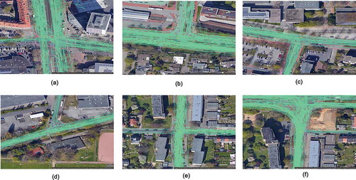
Six intersections from the city of Hanover, Germany, with different shapes (4-way and 3-way intersections), traffic rules (traffic lights, priority/yield signs, and uncontrolled intersections), and sampling density (number of trajectories that cross each intersection), were chosen for our analysis, as shown in Table 1. Two of them are 4-way and four are 3-way

Table 1. Number of trajectory samples (within parentheses) per intersection used in this study. With A, B, C, D, E, and F we distinguish the different intersections we use in our analysis

Intersection type	Traffic lights	Priority/Yield	Uncontrolled
4-way 3-way	A (148)		E (228)
	B (175)	C (68), D (48)	F (189)

intersections. Regarding their traffic-regulations, two are Traffic-light controlled, two Priority/Yield controlled, and two Uncontrolled (right-of-way rule). The data were recorded by a smartphone GNSS sensor with a frequency of 1 second. Each datapoint contains information about time (timestamp), position (latitude, longitude), speed and a unique identification number for each trajectory (trip). The data are naturalistic, as the driver of each trip (trajectory) was driving without any given instruction of how to drive or where to drive. The intersection crossings are all parts of daily traveling, such as routine driving from home to work. In Figure 1 are depicted the six intersections along with the trajectories that cross them.

Figure 1. Sample trajectories from the six intersections of the study. Source: Imagery © 2020 GeoBasis-DE/BKG, GeoContent, Maxar Techonologies, Map data © 2020 GeoBasis-DE-BKG (© 2009)

3.2. Trajectory clustering

The first objective of this study is to find the different paths that vehicles follow while crossing the intersections. This objective is a pre-requisite for the second objective. We assume as a path, a time-ordered sequence of locations that is followed by multiple trajectories. To find those paths, we apply trajectory clustering.

Trajectory clustering is a two-step process. First, the similarity of each trajectory with the others needs to be measured. Different measures can be used for assessing similarity (Zhang, Huang, and Tan 2006), such as Euclidean distance, Hausdorff distance, Fréchet distance, Dynamic Time Warping (DTW), and Longest Common Subsequence (LCSS), to mention some of them. We selected to test the Hausdorff distance, the Fréchet and DTW as they consider the direction of trajectories and they do not require the trajectories to have the same number of points (or length). Other methods do not distinguish between trajectories of different/opposite directions, that is trajectories from the same road but opposite directions are regarded to have a high degree of similarity. Moreover, as trajectories consist of a sequence of time-ordered GPS points (latitude, longitude, timestamp), they have a certain length and number of points. For practical reasons similarity metrics that can assess the similarity degree of trajectories independently of their length and/or number of points, are more convenient than methods that require the opposite. For these reasons, we selected to conduct our experiments by testing the Fréchet and DTW distance. The Hausdorff distance, additionally to the aforementioned advantages of Fréchet and DTW measures, is computationally very fast and for this reason it was selected for our comparison analysis. After computing the similarity of trajectories with each other, the next step is to find out groups of similar trajectories, in other words, to cluster them. There are various clustering techniques (Kisilevich et al. 2009), mainly categorized as direct, hierarchical, density-based, and graph-based. For our analysis, we test Agglomerative clustering and Affinity propagation (Xu and Tian 2015).

Agglomerative clustering (Müllner 2011) belongs to the Hierarchical Clustering family and follows the bottom-up principle. This clustering approach starts by considering each data point as a single cluster. In an iterative manner, the similarity measures are calculated between each cluster, and the most similar clusters are merged. The clustering process ends when all clusters are finally merged into a single cluster. This way a tree-like structure is obtained, called a “Dendrogram”. The clustering results are obtained by “cutting” the tree at either a specific height or number of clusters.

Affinity propagation (Thavikulwat 2008) is an unsupervised machine learning algorithm to cluster given data points, especially when the number of clusters is unknown. This clustering approach can be seen as a communication network, where every node sends a similarity message to each other node. The same way the responsibility answer to these messages is received at the sending node. Based on this communication structure, which is executed in an iterative way, the similarities are maximized for each set of data points and form the resulting clusters.

3.3 Movement behavior behavior analysis with speed- and time-profiles

The second objective of the study is to explore the behavior within each path (cluster of trajectories detected in the previous step) and find out how many different ways vehicles move along those same paths. We pursue this aim by clustering speed- and time-profiles of trajectories that follow the same paths. Since trajectories do not consist of the same number of GPS points, we segment them into equidistant segments of 1-meter length and interpolate the speed and timestamp values at the newly created points. From the intersection center, we select the parts of trajectories that are 50 meters before and 50 meters after the intersection center. That is, we select all trajectories that cross a certain intersection and consider for our calculations, parts of them that are exactly 100 meters long. In this way we generate speed-profiles, assuming that the intersection center is the point of reference for calculating the distance that vehicles travel, each of them consists of 100-speed values corresponding at every meter distant from the intersection center, starting from 50 meters before the intersection (denoted in Figures 2Figures 3, Figures4, Figures5, and Figures6 as negative distance the in x-axis), 49, 48, …, 1 meter and after the intersection, 2, 3, 4, …, 50 meters (positive distance in the x-axis of the aforementioned Figures). Similarly, we compute the time-profiles, where instead of speed we have time (assuming 0 seconds is the time when vehicle is 50 meters away from the intersection center). Having computed the feature vectors for clustering, we use the Fréchet distance as a similarity measure and the Affinity propagation algorithm for clustering the profiles.

Figure 2. The average performance of different similarity measures and clustering methods with 95% confidence level

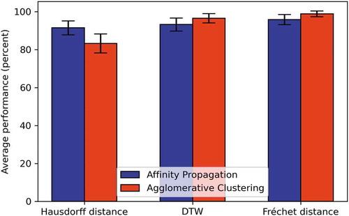
Figure 3. Clusters of speed ((a), (b), (c) and time (d) development from North to South at intersection A (traffic-light). 0 point in the x-axis, is denoted the intersection center. The negative distance denotes the distance (trajectory length) of the location of a vehicle from the intersection before the former crosses the junction center. Positive distance corresponds to the distance the vehicle has from the intersection center after it has crossed the intersection center

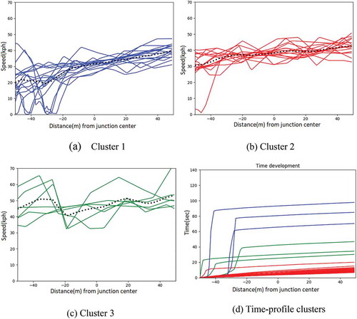
Figure 4. Clusters of speed ((a), (b), (c)) and time (d) development from East to West at Intersection B (traffic-light)

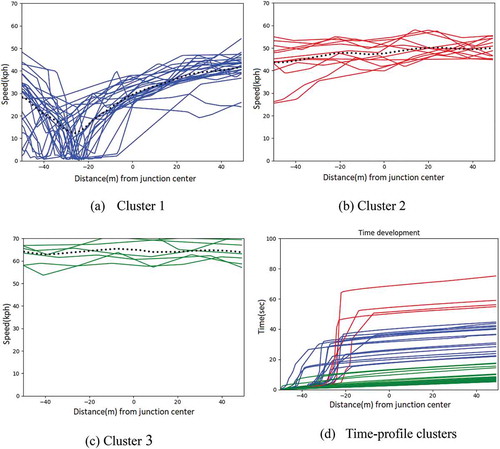
Figure 5. Different clusters of speed and time development at Intersection C from West to East (a, b, c), where a priority traffic-sign regulates the traffic and from South to West (d, e, f) where a yield-sign is valid. Similarly, plots g, h, i, j refer to Intersection D, from West to East, where vehicles have priority over other participants

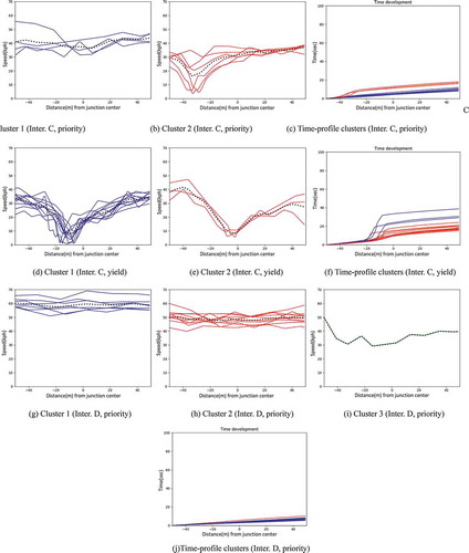
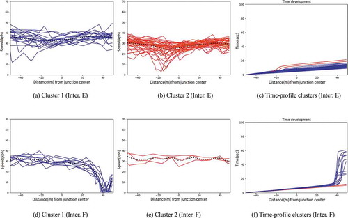
Figure 6. Different clusters of speed and time development at Inter. E from North to South and at Inter. F from South to North. Both junctions are uncontrolled (right-of-way priority rule)

4. Results

4.1. Results of trajectory clustering

Table 2 shows the trajectory clustering accuracy, defined as the correctly predicted cluster labels divided by the total number of cluster labels (total number of trajectories), under different settings: for different similarity measures and classification methods. In Figure 2 the average performance of the applied methods is also graphically depicted. From these results, we can infer that regarding the similarity measures, the DTW and Fréchet distance outperform the Hausdorff distance. Fréchet appears to have a slightly better performance than DTW. The computational complexity of Hausdorff has the advantage of being faster than the others.

Table 2. Clustering accuracy of the three tested similarity measures with 95% confidence level

	Affinity propagation			Agglomerative clustering
	Hausdorf	DTW	Fréchet	Hausdorf	DTW	Fréchet
A (traffic lights)	99% ±1.0	99% ±1.0	99% ±1.0	99% ±1.0	98% ±2.2	100% ±0.0
B (traffic lights)	95% ±3.3	95% ±3.3	96% ±2.9	92% ±4	93% ±3.8	100% ±0.0
C (priority/yield)	87% ±8.1	95% ±4.7	94% ±5.6	73% ±10.5	100% ±0.0	100% ±0.0
D (priority/yield)	88% ±9.4	82% ±11.1	91% ±7.9	83% ±10.6	90% ±8.7	100% ±0.0
E (uncontrolled)	89% ±4.1	95% ±2.8	97% ±2.3	60% ±6.4	99% ±1.1	99% ±1.05
F (uncontrolled)	91% ±4.1	93% ±3.6	98% ±2.1	93% ±3.6	99% ±1.3	94% ±3.4
Average performance	91.5% ±5.0	93.2% ±4.4	95.8% ±3.6	83.3% ±6.0	96.5% ±2.8	98.8% ±0.7

Regarding the clustering methods, Agglomerative is slightly better than Affinity Propagation, when combined with DTW or Fréchet. However, Agglomerative requires to set the number of clusters to be set in advance. This makes the Affinity propagation a preferable option for problems where such knowledge is given. Overall, we regard Affinity Propagation with the Fréchet distance measure as the optimal solution in the context of the problem we study, and for this reason, under these settings, we cluster the speed- and time-profiles, as shown in the next subsection.

4.2. Results of speed-, time-profile clustering

Figures 3 and Figures4 show the speed and time profiles of trajectories crossing Intersection A and Intersection B, both regulated by traffic lights. We can distinguish three patterns (clusters) in speed-profiles (for Intersection A: Figure 3(a–Figure 3c), for Intersection B: Figure 4(a–Figure 4c)), depicted in different plots and colors. The first cluster (blue) has low speed with stop(s) before the intersection center, whereas the other two clusters present an unhindered movement behavior while crossing the intersection. This mixed behavior observed at those locations is also highlighted in the time-profiles (Figures 3(d) and Figures4(d)), where clusters of different time/position development are observed. About 30 meters before the intersection center some vehicles stopped for 16–90 s, whereas others cross the intersection without any stop or speed adjustment.

Figure 5 shows the clustering results at Intersections C and D, which are priority/yield regulated. Regarding the priority regulation, we can see that at Intersection C, two clusters are observed (Figure 5(a,b)) one with unhindered behavior (5(a)) and the other (5(b)) with a deceleration event 30 meters before the intersection. At Intersection D (Figure 5(g–i)), all clusters represent unhindered movement at different speed levels (over 50kph, 40kph, and 30kph). Examining Intersection C, concerning the non-expected deceleration pattern along the priority roadway, we found that 30 meters before the intersection there is a pedestrian crossing and in front of that there is a traffic sign, warning the drivers of the upcoming crossing. This fact explains both the low average speed of the cluster with the unhindered behavior (Figure 5(a)) and that with the speed moderation for letting pedestrians pass the crossing (Figure 5(b)). This finding on the one hand highlights the validity of the method to detect movement patterns, on the other hand, it shows that when there are additional ruleswithin the observation site, the affected movement behavior as encoded in the speed-profile encompasses all the rules that influence the movement and not just the rule of the intersection control. Nevertheless, the stop behavior as depicted in the time-profile (Figure 5(f)) is of low-duration and follows the expected behavior when stopping at a pedestrian crossing.

Concerning the yield regulation, as can be seen in Figure 5(d and Figure 5e), vehicles either stop very close to the intersection center (about 10 meters before as shown in Figure 5(d)) or decelerate until almost stopped (Figure 5(e)). The speed at both clusters is below 40kph. Moreover, the duration of stop events due to yield is on average 18–20 s, which compared to the corresponding value at traffic lights is considerably shorter.

Lastly, the movement behavior at the uncontrolled intersections E and F is depicted in Figure 6. At such locations, we expect a low-speed movement, with short-duration stops if there is any traffic from the right and the driver must yield. Depending on the visibility of the roadway to the right, drivers regulate their speed accordingly. That is, when the visibility is good, as is the case in the examined intersections (Figure 1(e,Figuref)) where there is no building close to the intersection to “hide” the incoming traffic from the right, drivers may cross the intersection without decelerating for checking the traffic, as they can make the appropriate checks early before the intersection. In case of the low visibility of the traffic to the right, a deceleration or stop behavior is expected (similar to a yield sign). Nevertheless, no matter if the vehicles decelerate or not at an uncontrolled intersection, the crossing speed is lower (less than 40kph) compared to priority roadways (over 40kph). This means that uncontrolled intersections can be distinguished from priority/yield intersections, if we compare the speed at priority roadways with that at an uncontrolled location (even with very good visibility), as shown in the examples of Figure 6.

4.3. Can we infer traffic rules from speed-profiles?

From the analysis of the six intersections with different traffic rules, we can reflect on whether we can infer the traffic rules from speed/time-profile clustering. For any intersection type (three- or four-way), we should first check the time clustering result. If there are trajectories with stop time for over 20 s, the intersection can be inferred to be traffic light-regulated. In general, at this traffic rule, the collective behavior is expected to be a mixture of unhindered crossings, slight decelerated speed, and stops, where stops have a duration of 20–90 s. This expectation was validated from our analysis (Intersections A and B).

Uncontrolled intersections have the characteristic of low crossing speed. The visibility of the traffic to the right can define whether vehicles will decelerate or stop to check for traffic coming from the right. If the visibility is good, vehicles will only decelerate or stop to yield for other traffic participants crossing the intersection at the same time. If nobody comes from the right, the crossing will be unhindered. At an intersection of low visibility of the traffic to the right, vehicles will have to decelerate for the appropriate check of the traffic and stop only if there is traffic from the right. This means that there may be some uncontrolled intersections with a pattern combination of unhindered behavior, deceleration, and stop and some others with deceleration and stop pattern combination.

Given that at a yield sign, the same patterns are met as at low visibility uncontrolled intersection, we found that what can be distinctive between these intersection control types (uncontrolled and yield/priority signs), is the fact that the speed at uncontrolled intersections, no matter the visibility of the traffic to the right, is lower than that at locations with priority signs.

Due to limitations of the dataset, we did not have trajectories crossing the yield-controlled roadway of Intersection D, so we analyzed the yield category only based on the data from Intersection C. We consider this fact as a limitation of our study, as well as the fact that both examined uncontrolled intersections are of good visibility. It would be interesting to compare the results of the analysis of low and good visibility uncontrolled intersections. Another limitation of the study is the number of intersections per control type we have studied (two). Nonetheless, the fact that the results of the analysis validated the expectations we had on the possible movement patterns per control type, is encouraging regarding the effect that these limitations may have on the conclusions we drew from this small-scale analysis. We regard these findings as preliminary indications that speed and time profiles can be used for categorizing intersections according to traffic regulators in the context of a three-class classification problem, as examined in this study.

5. Conclusions

In this paper, we tested some similarity trajectory measures and clustering techniques for analyzing trajectories at intersections, using a dataset of six intersections from the city of Hanover, Germany. Regarding the similarity measures, we found that DTW and Fréchet distance performed better than Hausdorff, when dealing with bi-directional trajectory data, with Fréchet distance performing slightly better than DTW.

Concerning clustering methods, the comparison of Affinity propagation with Agglomerative clustering showed that the latter has somewhat higher accuracy than the former. With Agglomerative clustering, the number of clusters should be given by the user, which makes the approach less general than Affinity propagation. After that, clustering was applied to speed and time profiles sampled from the six intersections that are controlled by various traffic rules. The aim was to detect possible movement patterns and to examine whether they are indicative of the traffic controls that regulate the intersections.

To determine if an intersection is regulated by traffic lights, time-profiles seem to be more informative than speed-profiles, as they reflect the stop-duration of vehicles at those locations. The stop-duration at traffic lights is considerably longer than at other types of controlled intersections, so traffic lights can be distinguished by this characteristic. For the distinction between the other regulation categories, the results showed that speed profiles encompass all the required information needed for the scope. More specifically, we found that although movement patterns at yield and uncontrolled intersections share close similarities, on average the crossing speed of the movement patterns at uncontrolled intersections is considerably lower than that at priority-controlled intersections. This means that uncontrolled intersections can be distinguished from yield/priority intersections based on the average crossing speed. Priority from yield rules can then be easily identified as the observable patterns in speed-profiles are distinctive. We regard these findings as preliminary indications that speed and time profiles can be used for categorizing intersections according to traffic regulators in the context of a three-class classification problem.

Acknowledgments

The authors gratefully acknowledge the financial support from DFG.

Data availability statement

The data that support the findings of this study are openly available in Research Data Repository of the Leibniz University Hannover at https://data.uni-hannover.de, reference number https://doi.org/10.25835/0043786.

Additional information

Funding

This work is supported by the German Research Foundation (Deutsche Forschungsgemeinschaft (DFG)) with grant number 227198829/GRK1931.

Notes on contributors

Chenxi Wang

Chenxi Wang has received her M.Sc. degree in Computer Engineering from Leibniz University Hannover (Germany). Her research interests are trajectory analysis and pattern recognition.

Stefania Zourlidou

Stefania Zourlidou is a doctoral candidate at the Institute of Cartography and Geoinformatics, Leibniz University Hannover (Germany). She has received her M.Sc. degree in Intelligent Systems from UCL (London, UK). Her research interests include spatiotemporal analysis of crowdsourced data and machine learning.

Jens Golze

Jens Golze is a doctoral candidate at the Institute of Cartography and Geoinformatics, Leibniz University Hannover. He has received his M.Sc. in Geodesy and Geoinformatics from Leibniz University Hannover (Germany). His research interests include trajectory and laser scanning imaging analysis.

Monika Sester

Monika Sester is a Professor and Head of the Institute of Cartography and Geoinformatics at Leibniz University Hannover. She has received her PhD from the University of Stuttgart (Institute of Photogrammetry). Her research interests include geoinformatics, map generalization, spatial data integration and interpretation, spatial analysis and modeling, and machine learning.

Notes

1. physical features: final stop duration, minimum crossing speed, number of deceleration events, number of stops, distance of last stop from the intersection.

2. statistical features: minimum, maximum, mean, and variance of physical features.

References

- Åberg, L. 1998. “Traffic Rules and Traffic Safety.” Safety Science 29 (3): 205–215. doi:10.1016/S0925-7535(98)00023-X.
- Feng, Z., and Y. Zhu. 2016. “A Survey on Trajectory Data Mining: Techniques and Applications.” IEEE Access 4: 2056–2067. doi:10.1109/ACCESS.2016.2553681.
- Gudmundsson, J., P. Laube, and T. Wolle. 2008. “Movement Patterns in Spatio-temporal Data.” In Encyclopedia of GIS, 726–732. Boston, MA: Springer US.
- Hu, S., L. Su, H. Liu, H. Wang, and T. F. Abdelzaher. 2015. “Smartroad: Smartphone-based Crowd Sensing for Traffic Regulator Detection and Identification.” ACM Transactions on Sensor Networks 11 (4),:27.
- Hu, W., D. Xie, and T. Tan. 2004. “A Hierarchical Self-organizing Approach for Learning the Patterns of Motion Trajectories.” IEEE Transactions on Neural Networks 15 (1): 135–144. doi:10.1109/TNN.2003.820668.
- Jiang, B., D. Tian, Y. Tang, and D. Tao. 2018. “A Survey on Trajectory Clustering Analysis.” ArXiv Abs/ 1802: 06971.
- Junejo, I. N., O. Javed, and M. Shah. 2004 “Multi Feature Path Modeling for Video Surveillance.” Paper presented at the Proceedings of the 17th International Conference on Pattern Recognition, ICPR 2004, vol. 2, 716–719, Cambridge, UK, August 26–26.
- Kisilevich, S., F. Mansmann, M. Nanni, and S. Rinzivillo. 2009. “Spatio-temporal Clustering.” In Data Mining and Knowledge Discovery Handbook, 855–874. Boston, MA: Springer US.
- Kuntzsch, C., S. Zourlidou, and U. Feuerhake. 2016. “Learning the Traffic Regulation Context of Intersections from Speed Profile Data.” Paper presented at the Proceedings of GIScience 2016 Workshop on Analysis of Movement Data (AMD’16), Montreal, Canada, September 27.
- Makris, D., and T. Ellis. 2002. “Spatial and Probabilistic Modelling of Pedestrian Behaviour.” Paper presented at the Proceedings of the British Machine Vision Conference 2002, BMVC 2002, 1–10, Cardiff, UK, September 2–5.
- Makris, D., and T. Ellis. 2003. “Automatic Learning of an Activity-based Semantic Scene Model.” Paper presented at the Proceedings of the IEEE Conference on Advanced Video and Signal Based Surveillance, 183–188, Miami, FL, USA, July 22.
- Makris, D., and T. Ellis. 2005. “Learning Semantic Scene Models from Observing Activity in Visual Surveillance.” IEEE Transactions on Systems, Man, and Cybernetics, Part B: Cybernetics 35 (3): 397–408. doi:10.1109/TSMCB.2005.846652.
- Meneroux, Y., A. Le Guilcher, G. Saint Pierre, M. Ghasemi Hamed, S. Mustiere, and O. Orfila. 2020. “Traffic Signal Detection from In-vehicle GPS Speed Profiles Using Functional Data Analysis and Machine Learning.” International Journal of Data Science and Analytics 10 (1): 101–119. doi:10.1007/s41060-019-00197-x.
- Morris, T., and M. M. Trivedi. 2011. “Trajectory Learning for Activity Understanding: Unsupervised, Multilevel, and Long-term Adaptive Approach.” IEEE Transactions on Pattern Analysis and Machine Intelligence 33 (11): 2287–2301. doi:10.1109/TPAMI.2011.64.
- Müllner, D. 2011.“Modern Hierarchical, Agglomerative Clustering Algorithms.” CoRR. abs/1109.2378.
- Piciarelli, C., and G. L. Foresti. 2005. “Toward Event Recognition Using Dynamic Trajectory Analysis and Prediction.” Paper presented at the Proceedings of The IEE International Symposium on Imaging for Crime Detection and Prevention, ICDP 2005, 131–134, London, UK, June 7–8.
- Solomon, S., H. Nguyen, J. Liebowitz, and W. Agresti. 2006. “Using Data Mining to Improve Traffic Safety Programs.” Industrial Management and Data Systems 106 (5): 621–643. doi:10.1108/02635570610666412.
- Thavikulwat, P. 2008. “Affinity Propagation: A Clustering Algorithm for Computer-assisted Business Simulations and Experiential Exercises.” Paper presented at the Proceedings of The Annual ABSEL conference Developments in Business Simulation and Experiential Learnin g,Vol. 35, Charleston, South Carolina, USA, March 5–7.
- Xu, D., and Y. Tian. 2015. “A Comprehensive Survey of Clustering Algorithms.” Annals of Data Science 2 (2): 165–193. doi:10.1007/s40745-015-0040-1.
- Zhang, Z., K. Huang, and T. Tan. 2006. “Comparison of Similarity Measures for Trajectory Clustering in Outdoor Surveillance Scenes.” Paper presented at the Proceedings of the 18th International Conference on Pattern Recognition (ICPR’06), 1135–1138, Hong Kong, China, August 20–24.
- Zheng, Y. 2015. “Trajectory Data Mining: An Overview.” ACM Transactions on Intelligent Systems and Technology (TIST) 6 (3): 1–41. doi:10.1145/2743025.
- Zourlidou, S., C. Fischer, and M. Sester. 2019. “Classification of Street Intersections according to Traffic Regulators.” Paper presented at the Proceedings of the 22nd AGILE Conference on Geo-information Science, Limassol, Cyprus, June 17–20.
- Zourlidou, S., and M. Sester. 2019. “Traffic Regulator Detection and Identification from Crowdsourced Data—A Systematic Literature Review.” ISPRS International Journal of Geo-Information 8 (11): 11. doi:10.3390/ijgi8110491.