Quantification of the openness of urban external space through urban section

ABSTRACT

For the urban built environment, the shape characteristics of the external space are of decisive significance. However, what is commonly referred to as open space is more of a definition of social attributes. Therefore, in the research on urban environments, especially in urban microclimate, the study of a microclimate’s correlation with open space easily produces deviations. The identification of the openness of an external space based on a direct quantitative description is an important prerequisite for the cognitive urban form. In this study, based on the height-to-width ratio (HWR) of different directional sections of external space, areas with high openness in an urban space are extracted by the threshold value. In the case analysis of different areas in Nanjing, China, the results showed that the method is effective and convenient. The results of the analysis can also be used more widely in the urban design and research.

KEYWORDS:

• Urban external space
• urban section
• openness
• height-to-width ratio

1. Background

The urban form can be physically divided into two parts: objects and void (Akkerman 2009). The former includes buildings of various heights and volumes. The latter includes the space between the buildings, also called the urban external space. The external space is the spatial complementary set to buildings in the urban form.

The urban external space provides the public with both a variety of living activities and a variety of ground transportation sites and even a variety of abandoned or difficult-to-use venues (Jacobs 1992; Gehl 2011; Marzukhi, Karim, and Latfi 2012; Whyte 2012; Chen et al. 2015; Hahmann et al. 2018). Therefore, coverage of the urban external space is greater than the typical open space with which we are familiar. Open space refers to the space of entertainment, history, natural resource protection and other values and is a definition of social attributes (Turner 1992; Lynch 1995). The urban external space is the definition of physical attributes. All non-building parts of the city can be attributed to the external space. The shape characteristics of the external space play an important role in the urban ecological environment, human behavioral organization, and urban quality of life (Ford 2000). Especially important is that when we discuss the impact of the urban space on the urban microclimate (Erell, Pearlmutter, and Williamson 2012), it should refer to the urban external space of physical attributes rather than the open space of social attributes. More precisely, most of the research on the impact of urban open space on the microclimate is actually an external space with high openness. Therefore, studying the openness of an urban external space is of great significance. Spaces defined by the openness threshold of urban external spaces have the consistency of physical attributes, including the microclimate effect.

Compared with buildings, as a spatial complementary set, the shape of the urban external space is very complex, presenting a continuous but broken geometric character. The quantitative description of the urban external space can usually be divided into two levels: the overall and the local. Quantitative indicators of the overall urban external space include the fractal dimension (Chen 2013), porosity, occlusivity, and sinuosity (Adolphe 2001). Domingo, Thibaud, and Claramunt (2019) applied the graph-based approach to analyze the configurational structure of the external space network. These indicators focus on the overall characteristics of the spaces between the buildings. The research on the quantitative description of the local external space is concentrated in the streets and squares. Based on the section view, the height-to-width ratio (HWR) is a commonly used quantitative indicator of a spatial form (Ashihara 1983). In addition, many studies have focused on the two-dimensional morphological characteristics of local external space. Ding and Tong (2011) analyzed the definition of the street space profile from the perspective of visual perception. Hillier and Hanson (1989), Benedikt (1979), Batty (2001), and Othman, Yusoff, and Salleh (2020) combined the isovist analysis to map and quantified the visibility of the external space. Ji, Peng, and Ding (2019) adopted the area, shape, and openness to quantify the geometric characteristics of the external space. However, these indicators ignore the difference in building height.

Many researchers have verified the correlation between the three-dimensional geometrical attributes of an external space and the quality of the urban physical environment (Oke 1981; Chatzidimitriou and Yannas 2016; Fan and Liu 2018; Bouketta and Bouchahm 2020). The HWR of the street canyon, a typical external space, has an important correlation with the urban wind environment (Oke 1988; Li, Liu, and Leung 2009; Buccolieri, Sandberg, and Di Sabatino 2010; Lee and Kang 2015; He et al. 2017). Some researchers found that the geometric shape and orientation of streets have a strong influence on the microclimate of urban canyons by comparing the measured values with the simulation results (Kruger, Pearlmutter, and Rasia 2010; Andreou and Axarli 2012; Tsitoura, Michailidou, and Tsoutsos 2016). Chatzidimitriou and Yannas (2015) explored the influence of the HWR of the street canyon and street orientation on solar radiation, wind field, and pedestrian comfort using measured data and simulation analysis. In these studies of environmental quality involving an urban external space, most of the study objects are street canyons or squares with relatively clear boundaries. However, most of the street space in China is very blurred because of local planning regulations. Furthermore, for the entire city, the external space with clear boundaries is only a small number, and a large number of the boundaries of the external space are unclear.

From these studies, we also found that the HWR indicator is one of the most commonly used in the researches which involve the height information of the surrounding buildings. However, most studies only applied the HWR to evaluate the value of the enclosure of urban streets or squares. Moreover, only the HWR of the section line perpendicular to the road centerline was calculated (Alkhresheh 2007; Acre and Wyckmans 2015; Kaya and Mutlu 2017). Such a calculation cannot cover the city’s complex external spaces and only reflects the spatial characteristic in one direction but not in different directions of a three-dimensional space. Therefore, from the perspective of the urban section, this study used the HWR values in different directions of the external space as the basic data to measure the openness and divided the external space into different categories by setting the threshold value and visualizing different types of external spaces. The method could be applied for identifying and classifying the external spaces in complex urban environments.

2. Method

2.1. Generating distributed calculating points

The HWR is an important quantitative indicator of external space. When the external space is relatively regular, the calculated section of the HWR value is relatively easy to determine. When the external space is irregular, it is difficult to determine its calculated section. Therefore, this study first generated the distributed calculating points in the external space.

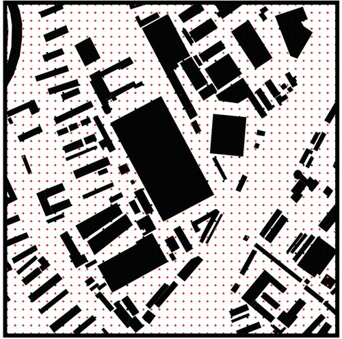
Factors affecting the generation of the points include point density, edge effects, and building avoidance. Figure 1 presents a plan view of a demonstration sample. First, we distribute the calculation points uniformly throughout the area. Obviously, some calculation points are inside the buildings, and these points should not be involved in the calculation. Furthermore, because this is only a slice taken from a larger urban area, its edges are not enclosed, causing some points on the edges to fail to calculate the HWR. To avoid such edge effects, in the calculation, we artificially add a wall to the edges. To simplify the calculation and reduce the impact of the additional wall on the calculation, we set the wall height to 1 m. Figure 2 presents the final calculation model and the points of the sample.

Figure 1. Distributed calculating points within a demonstration sample

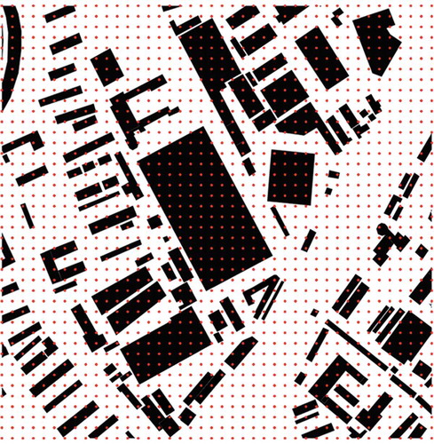
Figure 2. Final calculation model and the points

2.2. Calculating the HWR value of each considered point

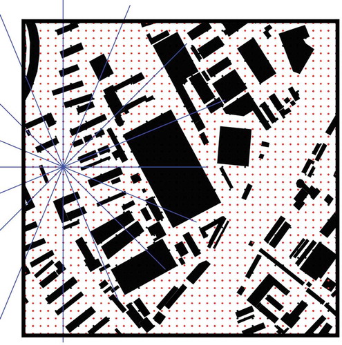
Considering the complexity of the shape of the external space, determining the section direction when calculating the HWR value is difficult. Therefore, we draw radiation lines in all directions that are centered on each calculating point to form a multidirectional section group and to calculate the HWR value in each direction. To balance the accuracy and time consumption of the calculation, we draw the radiation at intervals of 22.5° to obtain 8 section lines. Then, 8 HWR values can be calculated for each considered point (Figure 3).

Figure 3. The 8 section lines of one calculating point

In addition, two factors still need to be considered in the calculation of the HWR value. On the one hand, given the heterogeneity of urban buildings, the building heights on both sides of the calculating point are often unequal. Therefore, we use the average building heights on both sides for the HWR calculation. On the other hand, given the complexity of urban forms, in some areas with highly disparate building heights, the external space is not only the space between buildings but also the space above low buildings. Especially in a microclimate analysis, those higher buildings block airflow and sunlight far more than those low buildings and, thus, have a stronger influence on the calculation of the openness. Therefore, we need to scan all of the buildings on the section line and calculate the angle of the line between the calculating point and the top of each building section. On each side of the calculating point, the building with the largest angle is taken as the boundary surrounding the external space. Then, it is treated as the calculating buildings, and its height is used as the height in the HWR calculation. The distance between the two calculating buildings on both sides is the width in the HWR calculation. Figure 4 illustrates the taken buildings and the heights and width for the calculation.

Figure 4. Diagram to calculate HWR

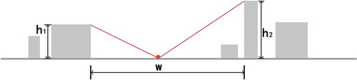
Then, the HWR calculation can be expressed as the following formula:

(1) $HWR=(h_1+h_2)/2w$(1)

where h₁ and h₂ are the heights of the buildings on both sides of the section line and w is the distance between the two buildings.

The value of the HWR can reflect the degree of openness of the external space in a certain direction where the calculating point is located. A larger value of the HWR results in a lower openness of the external space in the section direction. In contrast, a smaller value of the HWR results in a higher openness of the external space in this direction.

2.3. Identifying and outlining the external space with high openness

To identify the external space with high openness, we set several rules.

Rule 1: Set a threshold T. For each calculating point, when all of the HWR values of its eight directions are less than the threshold, the location of the point is an external space with high openness. Based on the different effects of the HWR on airflow (Oke 1988), T is set to 1/3.

Rule 2: For the distributed calculating points that meet Rule 1, connect the intersection of the different section lines and the calculating buildings on both sides to form the outline of the external space where the point is located.

For each calculation point that complies with Rule 1, we can draw its corresponding outline based on Rule 2. However, in some special linear spaces, such as roads and rivers, the section lines along the linear direction often do not have intersections until the boundary. At this time, the outline drawn with Rule 2 presents strong anisotropy, which affects the judgment of the external spaces. On the premise that the calculating points are evenly distributed, we hope that the external space obtained by each point appears clump-like to avoid being extremely narrow. Therefore, we further set the third rule.

Rule 3: When the building is far apart from the calculating point, the farthest distance FD is set as the end position of the outline. The FD can be determined according to the spacing of the distributed points and is usually set to a multiple of spacing.

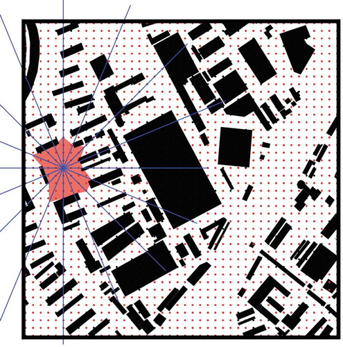
In Figure 5, the red polygon is an external space with the high openness of a calculating point in the sample area. Here, the FD is set at four times the spacing of the distributed points. Because the distance between most buildings is less than 8 times the spacing, we take half of it as the value of the FD.

Figure 5. Outlining the external space with high openness at a calculating point

Given the small distance between the calculating points, the calculated outlines overlap with each other. Of the entire study region, the superposition result of the area surrounded by all of these outlines is the final external spaces with high openness.

3. Case study

3.1. Characteristics of the case

Considering Nanjing as an example, we selected for study the range of four representative urban areas that are 3 km*3 km (Figure 6): Xinjiekou area, Hexi area, Chengnan area and Jiangning area. The relevant indicators of the four areas are shown in Table 1.

Table 1. Related indicators

Area	Plot ratio	Building density	Average building height (m)
Xinjiekou	2.522	0.304	24.880
Hexi	1.280	0.137	28.064
Chengnan	1.443	0.271	15.981
Jiangning	1.383	0.234	17.722

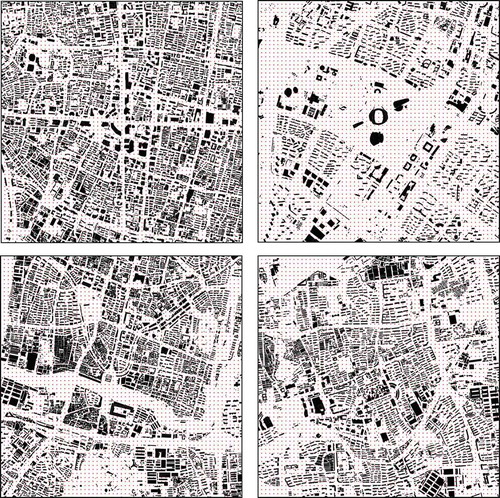
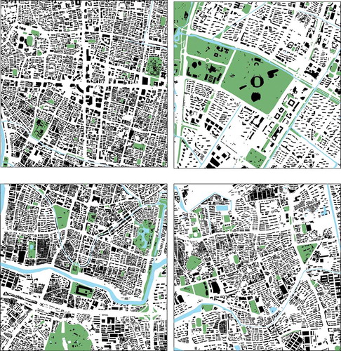
Figure 7 presents the plans of these four areas. Xinjiekou (Figure 7(a)) is the old central business district (CBD) of Nanjing city. The buildings in this district are high-rise, and the buildings’ volume ratio, density, and average height are the highest of the four areas. The urban texture can also reflect the characteristics of the city that is full of high-rise buildings. Located in the southwest of the main city of Nanjing, Hexi New Town (Figure 7(b)) is the new city center of Nanjing. Hexi New Town is a middle to high-end residential area with both residential and employment opportunities and a western leisure sightseeing area featuring riverside scenery. Compared with Xinjiekou, which is the old city center, the new city center has more external space, larger scale and lower building density. Chengnan, located in the Qinhuai District of Nanjing (Figure 7(c)), is the old city of Nanjing. As it is representative of the old city, the buildings have a small texture scale and a high density. The average building height is the lowest among the four areas. The Qinhuai River and the park along the river cross the area. The building density in Chengnan is not as high as that of the Xinjiekou area. Jiangning, located in the south-central part of Nanjing (Figure 7(d)), is in the suburbs of Nanjing. It is surrounded by the east and west sides of Nanjing and is an important hub for Nanjing’s external communication. The plot ratio and building density of the Jiangning area are higher than those in the Hexi area and lower than those in the Xinjiekou and Chengnan areas, and the average building height is only higher than that of the Chengnan area.

Figure 6. Selected research areas in Nanjing

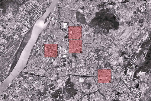
Figure 7. Plan of selected study areas. (a) Xinjiekou. (b) Hexi. (c) Chengnan. (d) Jiangning

3.2. Steps and threshold setting

In the research case, we used the API interface of the Baidu map and programming tools such as Python to obtain building data information for Nanjing. At the same time, we corrected the acquired artificial data to ensure their accuracy. Then, we imported the acquired data into the GIS software and edited the data in the GIS. Finally, we exported the vertex information and height information data files of the buildings in the selected area to the programming software for handling.

For the programming software, we used the Processing (https://www.processing.org) to handle our data. Processing is a software and programming language. It is free and is a flexible code language with good interactive capabilities  (Reas and Fry 2007). We use Processing to generate the city’s section data, preview the data in real time, and dynamically adjust them according to the results. In addition, we can also use the data to easily perform various statistical operations, such as computing and writing.

The Processing software reads the exported data and displays the plan. The red dots in Figure 7 are distributed calculating points. The spacing of the points is 50 m, and the number of points is 60 × 60. We set the number of cutting lines at each uniform point to 8 (the angle between the cutting lines is 22.5°). Then, the HWR values were calculated for every direction at each of the distributed calculating points.

To identify the external space with high openness, we followed the three rules mentioned in Section 2.3. The threshold T was set to 1/3. According to the distance between most buildings is less than 4 times the spacing, the FD is set at twice the spacing of the distributed points. The analysis results are shown in Figure 8.

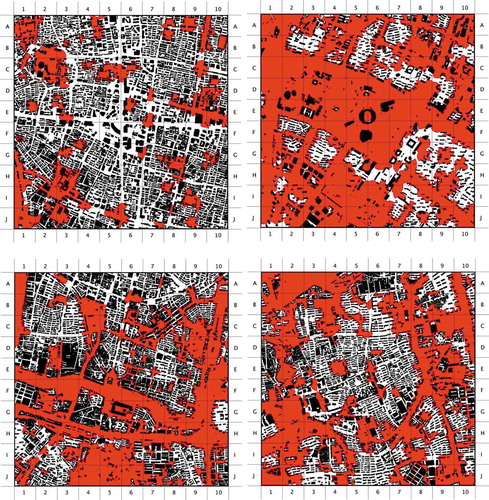
Figure 8. External spaces with high openness of the study area. (a) Xinjiekou. (b) Hexi. (c) Chengnan. (d) Jiangning

3.3. Calculation results of the case study

Table 2 shows the results of the calculations for the four areas. The results indicate that the proportion of the external space with high openness is from the Hexi block, Jiangning block, Chengnan area and Xinjiekou area.

Table 2. Calculation results for the external space with high openness

Name	Area (m^2)	Proportion
Xinjiekou	1,705,837	0.1895
Hexi	5,877,900	0.6531
Chengnan	3,329,803	0.3699
Jiangning	3,640,725	0.4045

Figure 8(a) shows the analysis results of the Xinjiekou area in Nanjing. Given the high density of buildings in the Xinjiekou area and the high-rise buildings, the external space that satisfies the conditions is scattered and presents a dotted layout. The large areas are concentrated in the Wutai Mountain area at 2B and 2 C, the Chaotian Palace area at 1I and 1 J, and the Presidential Palace Scenic Area at 9E.

Figure 8(b) shows the analysis results of the Hexi area in Nanjing. Given the relatively small building density in the Hexi area, two large parks – Olympic Center at 6E in the middle of the area and the Green Expo Park at 1A-1 J in the west – exist. In addition, the Nanjing International Expo Center is at 4 H, 4I and 5I. Therefore, the external space region that satisfies the set conditions in the Hexi region is large and extends from the center of the block to the outer region.

Figure 8(c) shows the analysis results of the Chengnan area in Nanjing. Given the high density of buildings in the old city, the external space that satisfies the conditions is mainly on the outside of the old city, such as the Qinhuai River Area (1A-1E-9 G-10B) and the parks along the river (such as Bailuzhou Park at 9D), the Saihong Bridge interchange at 1 G-9 H to the elevated area of the inner ring south line of the Shuangqiaomen Interchange, the Yuhuatai Scenic Area near 5 J on the south side of the area, and the unbuilt Taiheyuanzi community in 4B-4 C on the north side of the area.

Figure 8(d) shows the analysis results of the Jiangning area in Nanjing. As a suburb of Nanjing, many areas are currently under construction. Therefore, many unused sites are not completed and are distributed on the east side of the area. The external space that meets the set conditions is mainly concentrated in the Tushan Airport area on the northwest side (2-A, 3-A) and in the vicinity of the citizen park on the southwest side (2 G, 2 H).

We compare the four different texture areas and find that: (1) Xinjiekou and Hexi are the old center and the new city center of Nanjing, respectively. The proportion of the external space with high openness in Xinjiekou (0.1895) is much smaller than that of Hexi (0.6531). In addition, the layout of the external space with high openness is also very different: the number of external spaces with high openness in the Hexi area is large and distributed in a planar manner, whereas the number of external spaces with high openness in the Xinjiekou area is small and scattered. (2) The building densities of Xinjiekou and Chengnan are relatively close (0.304 and 0.271, respectively). However, given the high building height in Xinjiekou and the existence of the Qinhuai River and surrounding parks in the Chengnan area, the proportion of the external space with high openness in the Chengnan area is 0.3699, which is far more than the 0.1895 in the Xinjiekou area. (3) When comparing the Chengnan area with the Jiangning area, the plot ratio, building density, and vertical space with large openness are relatively close. However, the layout of the external space with high openness in the two areas is quite different: the external space with high openness in the south side of the city mainly presents a strip-shaped layout form on the Qinhuai River and the inner ring south line. The external space with high openness in the Jiangning area is distributed similar to the surface (2-A, 3-A Tushan Airport on the northwest, 2 G, 2 H citizen park on the southwest, and a large area of undeveloped land on the east side) and points.

3.4. Results analysis

The high-openness external space calculated in this study is significantly different from the traditional open space. Figure 9 shows the open space of the study case, including green space and water systems. Compared with Figure 8, the difference between them is obvious. Except for a few areas (i.e. 8-E in Xinjiekou, 9-B in Jiangning), the calculated result range is larger than the open spaces. The open spaces area ratios of Xinjiekou, Hexi, Chengnan, and Jiangning are 4.90%, 25.58%, 13.86%, and 7.25%, respectively. Compared with the values in Table 2, the open spaces area ratios are much smaller, especially in the newly developed area of Hexi and the suburb area of Jiangning. The definition of the external space with high openness using the method in the paper is different from the traditional definition of open space. The calculation results of the method are more meaningful for evaluating the microclimate in an external space. Taking advantage of these high-openness external spaces and expanding the area of open spaces will improve a city’s ecological environment.

Figure 9. Plan of green areas and water of the study area

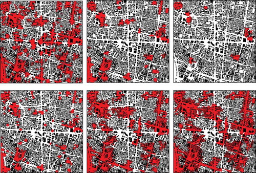
In addition, from the steps of the method, the two parameters T and FD have a strong influence on the result. The parameter T directly affects the judgment of the level of openness. The parameter FD directly affects the drawing of the final high openness external space.

Figure 10 shows the calculation results of the Xinjiekou area with different values of T and FD. The first row presents the results with different T values and the same FD value. The second row presents the results with the same T value and different FD values. Clearly seen is that an increase in the T value or the FD value results in an increase in the area of the calculated high-openness external space. However, the effect of the two parameters on the results is different. A larger T value results in a larger number of calculating points with high openness and vice versa. The change in the FD value does not affect the number of calculating points with high openness but has a significant effect on the area of each point. A smaller FD value results in a smaller area of high openness external space that tends to be circular. A larger FD value results in a larger area of high openness external space that tends to be star-shaped.

Figure 10. Results with different values of T and FD.

4. Conclusions and discussion

As a key element of urban sustainable development goals, open space has become the focus of urban planning and development. Generally, open spaces not only play a positive role in urban ecology but are also important in improving the urban microclimate. By evaluating the effects of the spatial patterns of green and other open spaces on the microclimate, urban planning and design can rationally improve the quality of an urban environment. In particular, in an important measure to improve the urban wind environment, open spaces are used to construct urban ventilation corridors. However, a large number of external spaces with high openness in contemporary urban space form still exist. They are not considered to be open spaces but have a significant impact on the urban microclimate. Therefore, from the perspective of the microclimate, considering only the setting of open space is not enough. This study analyzes the geometrical features of urban external spaces in a physical sense and proposes a method to quantify the openness of different locations. The method sets the distributed calculating points and then calculates the HWR values in multiple directional sections centered on each point. The statistics of the HWR values at each calculation point can be used as an indicator of the openness of the point. By this method, we can identify areas with high openness in a city’s external space.

This study applies this method and identifies high openness external spaces through analysis and calculation in different samples in Nanjing city. These spaces are clearly distinct from the open spaces usually defined by urban planning or management. Because its calculation process completely depends on the geometric features of the external space, its environmental quality is also more clearly related.

In another quantitative study of urban outer space, Kaya and Mutlu (2017) used a cellular-based method to calculate the 3D spatial enclosure of each cell and generated a spatial enclosure map of the study area. The enclosure here can be considered as the opposite of openness. In their research, they calculated the enclosure value of each cell and generated a raster map with different values. The raster map cannot directly display an external space with a lower enclosure. Even if some of the cells could be extracted through the threshold, the boundary of the cells lacks definition and meaning because it is separated from the building’s boundary. However, in this study, we used the intersections of the section lines with the building edges and the parameter FD to define the boundary of a high-openness external space. The results are more intuitive and suitable as study objects in an urban microclimate study.

The calculation process shows that the density of the distributed calculating points has an important influence on the results. If the density is too small, no calculating points may exist in some areas. If the density is too large, the calculation takes too much time. The density of the points also has a decisive influence on setting the parameter FD. Similarly, when calculating the HWR values of the sections through a considered point, the angular spacing of the sections also affects the results. A larger spacing results in a greater error in the representation of the surrounding situation. A smaller spacing results in more time being consumed. A reasonable distribution of calculating point density and section angle spacing needs to be determined on the basis of the study area.

When extracting areas of high openness, the determination of the threshold is also worthy of careful study. First, the threshold is determined by considering the city’s microclimate environment, including wind, temperature, and relative humidity. Second, the threshold of the HWR value calculated on the section lines in different directions should have a weight difference if the influence of the prevailing wind direction and the surrounding building orientation on the microclimate is considered. Finally, when outlining high-openness areas, if the building distance in a certain direction line is too far, the threshold set by Rule 3 also needs further study.

In general, as a preliminary study, the method still needs to be improved. However, this study provides a reference perspective for a quantitative analysis of urban external space. It also provides a reasonable method for studying the relationship between urban form and microclimate. Urban planning and design would optimize the open space system and improve the ecological environment based on a comprehensive understanding of the urban spatial form.

Disclosure statement

No potential conflict of interest was reported by the author(s).

Data availability statement

The data that support the findings of this study are available on reasonable request from the corresponding author.

Additional information

Funding

This research was funded by the National Natural Science Foundation of China [grant number 51578277] and the Major Program of National Natural Science Foundation of China [grant number 51538005].

Notes on contributors

Ziyu Tong

Ziyu Tong is an associate professor in School of Architecture and Urban Planning, Nanjing University. His research interests include computer aided architectural design, GIS and spatial analysis, urban morphology, and urban microclimate.

Huawu Yang

Huawu Yang is a graduate student in School of Architecture and Urban Planning, Nanjing University. His research interests include computer aided architectural design and urban morphology.

Chen Liu

Chen Liu is a graduate student in School of Architecture and Urban Planning, Nanjing University. His research interests include computer aided architectural design and big data analysis.

Tingting Xu

Tingting Xu is a graduate student in School of Architecture and Urban Planning, Nanjing University. Her research interests include architectural design and multi agent simulation.

Sha Xu

Sha Xu is a graduate student in School of Architecture and Urban Planning, Nanjing University. His research interests include computer aided architectural design, smart city, and big data analysis.

References

- Acre, F., and A. Wyckmans. 2015. “Dwelling Renovation and Spatial Quality: The Impact of the Dwelling Renovation on Spatial Quality Determinants.” International Journal of Sustainable Built Environment 4 (1): 12–41. doi:10.1016/j.ijsbe.2015.02.001.
- Adolphe, L. 2001. “A Simplified Model of Urban Morphology: Application to an Analysis of the Environmental Performance of Cities.” Environment and Planning B: Planning and Design 28 (2): 183–200.
- Akkerman, A. 2009. “Urban Void and the Deconstruction of Neo-platonic City-form.” Ethics, Place & Environment 12 (2): 205–218. doi:10.1080/13668790902863416.
- Alkhresheh, M. M. 2007. “Enclosure as a Function of Height-to-Width Ratio and Scale: Its Influence on User’s Sense of Comfort and Safety in Urban Street Space.” Gainesville, FL: Department of Urban and Regional Planning, University of Florida. Dissertation.
- Andreou, E., and K. Axarli. 2012. “Investigation of Urban Canyon Microclimate in Traditional and Contemporary Environment. Experimental Investigation and Parametric Analysis.” Renewable Energy 43: 354–363. doi:10.1016/j.renene.2011.11.038.
- Ashihara, Y. 1983. The Aesthetic Townscape. Cambridge, MA: MIT press.
- Batty, M. 2001. “Exploring Isovist Fields: Space and Shape in Architectural and Urban Morphology.” Environment and Planning B: Planning and Design 28 (1): 123–150. doi:10.1068/b2725.
- Benedikt, M. L. 1979. “To Take Hold of Space: Isovists and Isovist Fields.” Environment and Planning B: Planning and Design 6 (1): 47–65. doi:10.1068/b060047.
- Bouketta, S., and Y. Bouchahm. 2020. “Numerical Evaluation of Urban Geometry’s Control of Wind Movements in Outdoor Spaces during Winter Period. Case of Mediterranean Climate.” Renewable Energy 146: 1062–1069. doi:10.1016/j.renene.2019.07.012.
- Buccolieri, R., M. Sandberg, and S. Di Sabatino. 2010. “City Breathability and Its Link to Pollutant Concentration Distribution within Urban-Like Geometries.” Atmospheric Environment 44 (15): 1894–1903. doi:10.1016/j.atmosenv.2010.02.022.
- Chatzidimitriou, A., and S. Yannas. 2015. “Microclimate Development in Open Urban Spaces: The Influence of Form and Materials.” Energy and Buildings 108: 156–174. doi:10.1016/j.enbuild.2015.08.048.
- Chatzidimitriou, A., and S. Yannas. 2016. “Microclimate Design for Open Spaces: Ranking Urban Design Effects on Pedestrian Thermal Comfort in Summer.” Sustainable Cities and Society 26: 27–47. doi:10.1016/j.scs.2016.05.004.
- Chen, L., Y. Wen, L. Zhang, and W. N. Xiang. 2015. “Studies of Thermal Comfort and Space Use in an Urban Park Square in Cool and Cold Seasons in Shanghai.” Building and Environment 94: 644–653. doi:10.1016/j.buildenv.2015.10.020.
- Chen, Y. 2013. “A Set of Formulae on Fractal Dimension Relations and Its Application to Urban Form.” Chaos, Solitons & Fractals 54: 150–158. doi:10.1016/j.chaos.2013.07.010.
- Ding, W., and Z. Tong. 2011. “An Approach for Simulating the Street Spatial Patterns.” Building Simulation 4 (4): 321–333. doi:10.1007/s12273-011-0055-2.
- Domingo, M., R. Thibaud, and C. Claramunt. 2019. “A Graph-Based Approach for the Structural Analysis of Road and Building Layouts.” Geo-Spatial Information Science 22 (1): 59–72.
- Erell, E., D. Pearlmutter, and T. Williamson. 2012. Urban Microclimate: Designing the Spaces between Buildings. London: Routledge.
- Fan F., and Runping Liu. 2018. “Exploration of spatial and temporal characteristics of PM2.5 concentration in Guangzhou, China using wavelet analysis and modified land use regression model”. Geo-spatial Information Science 21 (4): 311–321.
- Ford, L. R. 2000. The Spaces between Buildings. Baltimore, MD: Johns Hopkins University Press.
- Gehl, J. 2011. Life between Buildings: Using Public Space. Washington: Island Press.
- Hahmann, S., J. Miksch, B. Resch, J. Lauer, and A. Zipf. 2018. “Routing through Open Spaces – A Performance Comparison of Algorithms.” Geo-Spatial Information Science 21(3): 247–256.
- He, L., J. Hang, X. Wang, B. Lin, X. Li, and G. Lan. 2017. “Numerical Investigations of Flow and Passive Pollutant Exposure in High-Rise Deep Street Canyons with Various Street Aspect Ratios and Viaduct Settings.” Science of the Total Environment 584: 189–206. doi:10.1016/j.scitotenv.2017.01.138.
- Hillier, B., and J. Hanson. 1989. The Social Logic of Space. Cambridge: Cambridge University Press.
- Jacobs, J. 1992. The Death and Life of Great American Cities. New York: Vintage.
- Ji, H., Y. Peng, and W. Ding. 2019. “A Quantitative Study of Geometric Characteristics of Urban Space Based on the Correlation with Microclimate.” Sustainability 11: 4951.
- Kaya, H. S., and H. Mutlu. 2017. “Modelling 3D Spatial Enclosure of Urban Open Spaces.” Journal of Urban Design 22 (1): 96–115. doi:10.1080/13574809.2016.1235465.
- Kruger, E., D. Pearlmutter, and F. Rasia. 2010. “Evaluating the Impact of Canyon Geometry and Orientation on Cooling Loads in a High-Mass Building in a Hot Dry Environment.” Applied Energy 87 (6): 2068–2078. doi:10.1016/j.apenergy.2009.11.034.
- Lee, P. J., and J. Kang. 2015. “Effect of Height-to-Width Ratio on the Sound Propagation in Urban Streets.” Acta Acustica United with Acustica 101 (1): 73–87. doi:10.3813/AAA.918806.
- Li, X. X., C. H. Liu, and D. Y. Leung. 2009. “Numerical Investigation of Pollutant Transport Characteristics inside Deep Urban Street Canyons.” Atmospheric Environment 43 (15): 2410–2418. doi:10.1016/j.atmosenv.2009.02.022.
- Lynch, K. 1995. City Sense and City Design: Writings and Projects of Kevin Lynch. Cambridge, MA: MIT Press.
- Marzukhi, M. A., H. A. Karim, and M. F. Latfi. 2012. “Evaluating the Shah Alam City Council Policy and Guidelines on the Hierarchy of Neighborhood Open Space.” Procedia-Social and Behavioral Sciences 36: 456–465. doi:10.1016/j.sbspro.2012.03.050.
- Oke, T. R. 1981. “Canyon Geometry and the Nocturnal Urban Heat Island: Comparison of Scale Model and Field Observations.” Journal of Climatology 1 (3): 237–254. doi:10.1002/joc.3370010304.
- Oke, T. R. 1988. “Street Design and Urban Canopy Layer Climate.” Energy and Buildings 11 (1–3): 103–113. doi:10.1016/0378-7788(88)90026-6.
- Othman, F., Z. M. Yusoff, and S. A. Salleh. 2020. “Assessing the Visualization of Space and Traffic Volume Using GIS-Based Processing and Visibility Parameters of Space Syntax.” Geo-Spatial Information Science 23(3): 209–221.
- Reas, C., and B. Fry. 2007. Processing: A Programming Handbook for Visual Designers and Artists. Cambridge, MA: MIT Press.
- Tsitoura, M., M. Michailidou, and T. Tsoutsos. 2016. “Achieving Sustainability through the Management of Microclimate Parameters in Mediterranean Urban Environments during Summer.” Sustainable Cities and Society 26: 48–64. doi:10.1016/j.scs.2016.05.006.
- Turner, T. 1992. “Open Space Planning in London.” Town Planning Review 4: 365–385. doi:10.3828/tpr.63.4.l703v67051278442.
- Whyte, W. H. 2012. City: Rediscovering the Center. Philadelphia: University of Pennsylvania Press.