Modeling relationships between the network distance and travel time dynamics for assessing equity of accessibility to urban parks

ABSTRACT

Static models of accessibility are usually based on the fixed distance or Average Travel Time (ATT) models. Because of ignoring the traffic as a dynamic process affecting the accessibility through the change of Travel Time (TT), these models lead to unperceived temporal inequities. In contrast to the consideration of the temporal Variation of TT (VTT) in the previous studies, the variation of traffic-related TT and its relations with network distance has not been considered. In this study, relations between VTT and network distance to access urban parks in Tehran megacity has been modeled. Traffic maps at five times of day are used to produce TT maps of Traffic Analysis Zones (TAZs) to their 3-closest parks. Comparison of the Gini coefficients of accessibility show significant inequities of accessibility at different times of day. Relations between the distance, ATT, and TT_max are modeled by statistical analysis. Results show both TT and TT_max have significant positive relations with distance and traffic and reach their maximum at 6 p.m. Observation of significant relations between distance, ATT, TT_max, and VTT provides interesting knowledge for the conversion of temporal measures of equity (TT) to a physical measure of equity (distance). A simple application of these findings for effective management of the spatiotemporal inequities is the definition of critical distances from public services. As an example, to decrease the TT_max of TAZs to less than 12 min, their maximum distance to the closest parks should be less than 4 km. The developed approach can be adopted for the accessibility evaluation of the other public services, particularly the health and education centers.

KEYWORDS:

• Spatiotemporal equity
• accessibility
• travel time variability
• Gini coefficient
• Lorenz curve
• urban parks
• Tehran megacity

1. Introduction

Sustainable urban development is one of the most significant objectives of urban planners and managers. The UK Government’s definition of sustainable development relates to a better quality of life for individuals (Berke and Manta 1999; Choi and Ahn 2013). One of the key objectives of smart urbanism is to encourage spatial equity through equal access to affordable housing, economic activities, services, and facilities (El Din et al. 2013). So, accessibility is a key concept in assessing spatial equity in the distribution of services across the world (Van Wee 2016) and realizing sustainable urban development.

There are three principal components for measuring accessibility, including the destination of the travel, the origin of the travel, and the access cost from the origin to destination points (Bhat et al. 2002). Regardless of the fact that spatial accessibility is a dynamic concept in time, it has been often treated as a static concept in previous studies. In these studies, access costs to services are defined by a static Euclidean or network distances between a service recipient and a service provider. Although the physical distances between pairs of points remain constant, their access costs depend on travel time and traffic circumstances over different periods of time.

Considering time and space as the important parameters in the assessment of spatial equity of accessibility provides a four-dimensional space of analysis. Fixed and variable assumptions of location and time form a quadruple space of analysis as in Figure 1.

Figure 1. Four-dimensional space of analysis of the spatial equity of accessibility

First-quarter is based on a fixed time and location, which is only valid for a single location at a given time. The second quarter assumes a single-time and uses variable locations for the assessment of equity as has been usually used in most of the previous studies. The third quarter is based on analysis of the accessibility while both dimensions of location and time are variable. This can be regarded as the most realistic space of analysis. Finally, the fourth quarter examines the accessibility of a single location during the time-varying conditions.

In reality, TT shows high variability because of the dynamics of traffic conditions in urban environments. Therefore, the problem of inequity caused by the temporal Variability of the TTs (VTTs) to public facilities is an important aspect that deserves special considerations. Particularly, an examination of relations between the spatial and temporal inequities can lead to more in-depth information about the inequities, effects of inequity on the quality of life of residents, and how they can be managed and controlled. Because of the higher risk of traffic at longer distances, spatial and temporal accessibilities are expected to show complex behaviors. This means residents located at higher distances from public services are exposed to higher VTTs in a given distance.

The problem of dynamic TTs has recently been addressed by some researchers. However, relations between distance and TT have not been considered and deserve careful considerations. Distance and time are the most frequently used parameters for measuring the equity of accessibility. Since distance is usually used as an access indicator in urban planning tasks, the development of models between TT and distance can provide valuable knowledge for the transformation of TT to distance, leading to a more precise definition of access time and the access distance standards in the planning process. Therefore, an important aim of this research is to model the relations between spatial and temporal access to urban parks, as an example of public services. The primary questions that are answered in this research are “How accessibility varies with time and how are spatial and temporal accessibilities related?” The Lorenz curve and the Gini coefficient are also used to determine how fair the accessibility is at different locations and times of the day.

The rest of the paper is organized as follows: Section 2 reviews previous literature on this topic; section 3 briefly introduces the methods of the study; section 4 introduces the study area and describes the modeling results of the relationships between the network distance and TT dynamics. Results of assessing the dynamics of spatial and temporal inequity of accessibility to urban parks and the application of the results for the management of the spatial and temporal inequity in the Tehran megacity as the case study area are also included in section 4. In Section 5 the conclusion of the research is put forward.

2. Literature review

A review of the previous works shows that the prime focus of many of the previous studies has been in the second quarter of the analysis space, and a few studies have addressed the third quarter as outlined in Figure 1. As an example, Mansour (2016) assessed the spatial pattern, distribution, and provision of public health services using distances from demand points to providers extracted from the near analysis. In another study, Kompil et al. (2019) proposed a novel approach to map generic service accessibility in Europe. This approach was used to compare average distances to services and the number of residents who can walk or cycle to access the services in urban and rural areas. This study used the average distance at a fixed time to estimate and compare the accessibility of different regions and ignored the considerable differences between the travel distances and TTs. Similar ignorance can be found in some other studies (e.g. Lucy 1981; Talen 1997; Talen and Anselin 1998; Nichols 2001; Pasaogullari and Doratli 2004; Tsou, Hung, and Chang 2005; Omer 2006; Oh and Jeong 2007; Liao, Hsueh-Sheng, and Tsou 2009; Lotfi and Koohsari 2009; Zhang, Hua, and Holt 2011; Taleai, Sliuzas, and Flacke 2014; Ye and Xiang 2015; Dadashpoor and Rostami 2017; Kimpton 2017; Wu et al. 2017; Wen et al. 2018; Arranz-López, Soria-Lara, and Ángel 2019).

Some studies have considered TT instead of the travel distance for measuring spatial accessibility. For example, Fotini (2017) measured the individual accessibility to daily activities during a typical day, using an additional factor of activity space along with the places of activities, time, and temporal constraint. By considering different travel modes for quantifying accessibility as distances and TTs, Salonen (2014) analyzed the spatial patterns of realistic accessibilities to services. A similar study has been completed by Zhang et al. (2019) to assess the level of equity of access to community-based services. They assessed the accessibility of Chinese older adults by considering the frequency of using four travel modes of walking, cycling, bus-riding, and driving. In this study, the Average Nearest Neighbor (ANN) method was used to get the characteristic of the geographical distribution of community-based service centers. They finally proposed an alternative method to measure the accessibility of older adults by considering their travel behaviors. Tahmasbi et al. (2019) presented a multimodal accessibility-based equity assessment using the required TT for walking, using private cars or public transportation modes to access urban public facilities. In this study, the estimation of accessibility was based on the average values of TTs between the origins and destinations. Chang and Liao (2011) used the network and straight distances to show the role of mobility on the spatial equity of services and developed an integrated framework composed of two models of accessibility and mobility for measuring the spatial equity. Cheng et al. (2016) analyzed the spatial variation of medical centers and the accessibility to hospitals using TTs. Both the TTs of driving and using public transportation were computed and their mean values were used in the analysis. Lawal and Anyiam (2019) examined geographic access to Primary Health Care Facilities (PHCF) in Nigeria, using the average TT from settlement areas to PHCFs. Results showed that more than 98% of the settlements have good access (less than 30 min), whereas, others are located in the poor (31–60 min) and very poor (over 60 min) access classes. Although the mentioned studies have used TTs instead of the travel distance and have enhanced the spatial equity measurement by considering different travel modes, the dynamic nature of TTs and the resulting impacts on the accessibility has not been well considered.

Some recent works have addressed the instant TTs and their dynamics for estimating Spatiotemporal accessibility and equity. As an example, Stępniak and Goliszek (2017) analyzed the spatial and temporal variation of accessibility to public transport in Szczecin (Poland). They analyzed the variation of TTs during a day using the averaged 15-min-long time periods. Results showed that some neighborhoods were affected by the high daily variation of accessibility and the low average accessibility values, which is called the “double-affected” issue. Hu et al. (2018) used a simulation model of traffic flow based on a macro-traffic simulation for estimation of TTs in various time periods during the day under free-flow and congested road conditions. The spatial accessibility of emergency medical services (EMS) in inner-city Shanghai was analyzed and classified into 5 different groups of accessibility (Q1-Q5), where Q5 represented the most deprived group in which the EMS cannot provide service in less than 8 min. Then, the accessibility of the area and number/percentage of the population in the Q5 were further analyzed during different times of the day. García-Albertos et al. (2019) used mobile phone records for constructing origin to destinations (OD) travel matrices to examine different scenarios for dynamic accessibility analysis. They examined four scenarios that included 1-the reference scenario based on the mean TT and destination attractiveness, 2 – the dynamic congestion scenario using the variable instant TTs and static destination attractiveness, 3- the dynamic attractiveness scenario based on the variable destination attractiveness and mean TT and finally 4- the dynamic accessibility scenario using the variable instant TTs and variable destination attractiveness. The analysis was conducted in three-time slots, including the morning peak, off-peak, and the evening peak. Results indicated that geo-located data can provide more accurate and realistic information than static or partially dynamic analyses. Zheng et al. (2019) considered the dynamic changes in transport costs to hospital services using public transit and self-driving modes of transportation. Instant TTs to access hospital services were considered at the peak and off-peak traffic hours of the day. Then, four baseline indicators including the minimum, maximum, average, and optimal weighted models of TTs were developed and analyzed to measure the accessibility of each residential area to hospitals. Supply and demand of the urban green spaces and their accessibility by elderlies in Salzburg (Austria) were studied by Artman et al. (2019). This study mainly focused on actual distances and barriers to reach and use green spaces by elderlies. Results of supply analysis showed the availability of green spaces in distances between 500 and 1000 m. But because of the existing barriers and difficulties of access for old-aged users, they prefer to use green spaces outside the service areas.

3. Methods

3.1. Accessibility measure

Gravity model as one of the most useful approaches for spatial equity measurement of accessibility is used in this study (Makri and Folkesson 1999). This model is based on the spatial interaction model and accessibility index measurement and considers both aspects of access costs and benefits, respectively expressed as the distance (or time) and attractiveness indices. The time-based accessibility index of this model can be expressed as:

(1) ${\alpha }_i^l\left(t\right)={\sum }_{j=1}^n\left(w_j^l\times ex{p}^{\left(-t_{ij}^l\left(t\right)\right)}\right)$(1)

where i and j are counters for recipients and services, respectively, ${\alpha }_i^l\left(t\right)$ is the index of accessibility of parcel i as a recipient to an urban service of type l at time t, $n$ is the number of services of type l in the neighborhood of the parcel i, $w_j^l$ is the attractiveness index of service j and $t_{ij}^l\left(t\right)$is the TT from the recipient i to service j at time t.

The attractiveness index of service j depends on its capacity and quality and also the number of service users. Because of the lack of useful information about the capacity and quality of public service centers, particularly the parks, their size can be used as the representative of their capacity and quality. By assuming a negative linear relationship between the attractiveness index and the number of demanding users of a service center, attractiveness index of a service center can be modeled as a function of its size (area) and the demanding population who prefer to visit service j:

(2) $w_j^l=S_j^l/P_j^l$(2)

where

(3) $P_j^l={\sum }_{i=1}^{I}Po{p}_i$(3)

in which $S_j^l$ is the area of service j of type l, $P_j^l$ is the total population who prefer to use service j and $Po{p}_i$ is the population of TAZ _i who visit service j.

3.2. Spatial and temporal accessibility relations

If the influences of other parameters such as accidents and car breaks-downs in urban areas are ignored, traffic plays the most important role in the definition of TT from a recipient such as i to service j. Therefore, TT is a dynamic parameter that varies at different times of a day due to different traffic conditions and speeds of movement. If the average speed of movement in different routes from origins to the closest service centers is represented by $V_{\mathrm{a}\mathrm{v}\mathrm{g}}$, then the average TT (ATT) from location i to j can be expressed as:

(4) $AT{T}_{ij}=V_{avg}\times d_{ij}$(4)

where $d_{ij}$ represents the distance from the location i to j. Instant TT (ITT) in a given time can be expressed as:

(5) $IT{T}_{ij}=AT{T}_{ij}+VT{T}_{ij}$(5)

where $VT{T}_{ij}$ represents the variability or errors of estimating ITT by ATT and can take positive or negative values. This means that ITT can be described by two components. One is the ATT, a systematic component which is the linear function of distance. Another one is the VTT which is a function of both distance and traffic and varies with time and traffic conditions. ITTs of different routes can be estimated using the real-time traffic maps, data of traffic sensor networks, and other related available information from the internet networks. By assuming ATT as the linear function of distance, this parameter can be estimated by collecting representative samples of daily traffic conditions and fitting a linear model between the distance of all the origins from their destination service centers and ITTs of different sample traffic conditions.

(6) $AT{T}_{ij}=f_1\left(d_{ij}\right),orAT{T}_{ij}=a\times d_{ij}+b$(6)

By calculation of the difference between the ITT and ATT, VTT for each route, distance and time can be estimated from:

(7) $VT{T}_{ij}=IT{T}_{ij}-AT{T}_{ij}$(7)

Because of the spatial autocorrelation effects, closer areas are expected to be more similar than the farther places. So, it is expected that diversity of traffic, car speed, and route conditions increase with the distance, resulting in an increasing trend of VTT with the distance. Then VTT for each distance and time can be estimated by modeling the relations between the distance and VTT.

(8) $VTT=\hspace{0.17em}{f}_2\left(d\right)$(8)

and ITT can be represented as a function of distance:

(9) $ITT=f_1\left(d\right)+\hspace{0.17em}{f}_2\left(d\right)$(9)

Different statistical properties of TT and VTT such as the maximum, minimum, and average values for different time periods can be estimated and used in the assessment of access equity in different distances and times. As an example, maximum values of TT (TT_max) in a given time period is an important criterion which is usually intended to be minimized or preferred to be less than a certain threshold in equity assessment and planning. This parameter for each distance can be estimated from:

(10) $T{T}_{\mathrm{m}\mathrm{a}\mathrm{x}}=ATT+VT{T}_{\mathrm{m}\mathrm{a}\mathrm{x}}=f\left(d\right)$(10)

So, modeling of ITT and TT_max as a function of distance, as in equations 9(9) $ITT=f_1\left(d\right)+\hspace{0.17em}{f}_2\left(d\right)$(9) and 10(10) $T{T}_{\mathrm{m}\mathrm{a}\mathrm{x}}=ATT+VT{T}_{\mathrm{m}\mathrm{a}\mathrm{x}}=f\left(d\right)$(10) , can lead to the transformation of time to distance and effective management of both the spatial and temporal inequities.

3.3. Access equity assessment

Measuring the accessibility only makes a visual index over the specified spatial units, and it does not show the equity of distribution of services (Guzman, Oviedo, and Rivera 2017; Lucas, van Wee, and Maat 2016; Neutens et al. 2010; Van Wee and Geurs (2011)). Among the existing indices, the Lorenz curve, and the Gini coefficient as the scale-independent indicators have gained a broad application (Xu et al. 2018).

In this study, the Gini coefficient is applied to measure the level of the inequity of the accessibility at different times of the working day. The difference between the Gini coefficients got at different times of the day can show the effects of urban traffic on the equality of access to services during the day. The Gini coefficient is equal to the ratio of the area of the gap between the Lorenz curve and the 45-degree line of complete equality over the total area under the line of complete equality (Shirmohammadli, Louen, and Dirk 2016) (Equation 11(11) $GC=1-{\sum }_i\left(Y_{i+1}+Y_i\right)\left(X_{i+1}-X_i\right)$(11) ).

(11) $GC=1-{\sum }_i\left(Y_{i+1}+Y_i\right)\left(X_{i+1}-X_i\right)$(11)

where GC is the Gini coefficient value, $Y_i$ is the cumulative proportion of the accessibility and $X_i$ is the cumulative proportion of the population in the study area (Tahmasbi et al. 2019; Brown 1994; Welch and Mishra 2013). In this paper, the accessibility index is measured for each TAZ and the total population of each TAZ is considered as $X_i$ in the Gini coefficient equation. GC value equal to zero and one respectively indicates perfect equality and perfect inequality in accessibility among TAZs.

4. Practical experiments and results

4.1. Case study area

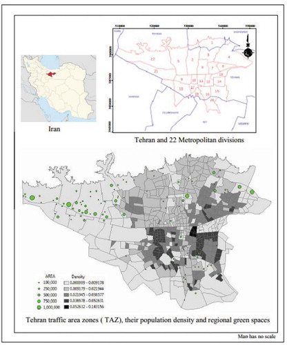
The case study area is the Tehran megacity, the capital of Iran. Tehran is divided into 22 metropolitan regions. Each region is divided into several districts, and, finally, each district includes several local neighborhoods. In the latest official national census in 2016, Tehran had a population of 8,737,510 extended in about 640 square kilometers. The city is divided into 560 TAZs which are treated as the service demanders in this study (Figure 2).

Figure 2. Green space distribution and geographic location of the Tehran megacity as the case study area

4.2. Distribution and supply of green spaces

Green spaces in the study area show uneven patterns of distribution. Correlation analysis of population and park area density in TAZs shows inverse relations between these two; with low population density TAZs having higher park area densities, especially in the western parts of the city (Figure 3). This may be because of the larger size and number of available bare lands and open spaces in the western parts of Tehran (regions 21 and 22). Also, the construction of Lunar Cities around the city for the accommodation of the overflow population of Tehran has led to higher park densities in these regions. This has resulted in a higher number of extensive parks in fewer populated areas, while most of the small parks are located in densely populated areas (Figure 3).

Figure 3. Relations between population density (horizontal axis) and park area density (vertical axis) in the study area

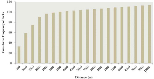
Distribution of the number of parks as the supply source in different distances from the TAZs as the demanders is highlighted in Figure 4. As seen, about 50% (59 parks from the total of 114), are located in distances less than 1,000 m from the TAZs, and the most parks (about 85% of parks, 97 from 114) can be reached in less than 3,000 meters distance from the TAZs. The number of existing parks shows sharp increases from 500 to 2500 m. After this, an increase in the distance leads to a minor increase in the number of parks from 97 to 114. Only 33 parks that are about 29% of the existing parks are in distances closer than 500 m. On the other hand, as highlighted in Figure 3, inverse relations between the park and population density lead to the intensive occupation, and therefore, lower attractiveness of parks in populated areas. So, the situation of accessibility and attractiveness from the supply side, particularly for children and elderly people, is well below the acceptable levels, and accessibility by driving a car is the usual practice.

Figure 4. Cumulative frequency of parks located in different distances from TAZs in the study area

4.3. Travel distance and TT estimation

Measuring access to services has two principal elements: the service provider and the service receiver. In this paper, Tehran traffic analysis zones and the urban parks have been considered as the service receivers and providers, respectively. The Network Analyst, OD (origin-destination) Cost Matrix tool of ArcGIS has been used to measure network travel distances between TAZs and urban parks with considering length as the impedance function. Due to the lack of reliable data on the exact location of city park entrances, centroids of TAZs and urban parks have been used as the origins and destinations, respectively.

To avoid limitations caused by assuming each service user to choose only one service, in this study, the spatial accessibility of TAZs to their three nearest parks has been analyzed. Considering several adjacent services instead of the nearest one can be of particular interest in the assessment of the access equity to the alternative parks in a larger context. As an example, two residents may have equal distances from their first closest parks, whereas they may have different access to the alternative parks because of the differences in their distances from the second and third closest parks.

One of the important objectives of this study has been to estimate, and map TTs of all TAZs to the three closest parks at five different times of the working day. So, because of the need for spatial data of traffic conditions, numerous TAZs and OD points, and also spatially continuous and real-time data of traffic conditions provided by the Google Maps, these maps have been used as the source of traffic data. Traffic maps provide detailed spatial and temporal information on traffic conditions, which can be useful for mapping and understanding the spatial patterns of traffic conditions and their effects on distance-time relationships.

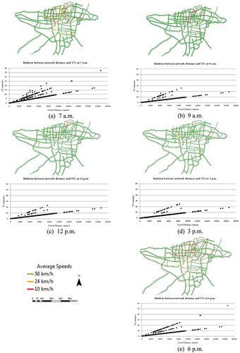
Real-time traffic conditions of the study area were monitored and gained for five samples of varying traffic conditions during the working day times at 7 a.m., 9 a.m., 12 p.m., 3 p.m., and 6 p.m., using the Google Maps. Different traffic patterns and representativeness of these times were the main reason for their selection. In Google traffic maps, street segments are constantly labeled with three traffic classes named “Light”, “Moderate” and “Heavy” which are respectively equivalent to maximum speeds of 80, 50 and 30 km/h according to the local traffic control agencies. For the computation of travel time in different ODs, the existing web-based local route planning tools based on the Google Maps were used to calculate the average speeds in each of the three traffic classes. These respectively resulted in average speeds of 10, 24, and 58 km/h for the heavy, medium, and light traffic classes. Then the calculated average speeds and traffic maps of five different times were used to compute the total TTs for ODs by measuring and summation of the TTs of different segments of the networks connecting each TAZ to the three closest parks.

4.4. Relationships between distance, TT and VTT

Evaluation of relations between distance and TT are mainly based on the use of public or private cars. The principal reason for this choice is the scattered patterns of park distribution, acute sensitivity of this transportation mode to traffic conditions, and its frequent use to access parks in the study area.

Results of examining relations between the network distance and TT at five sample times of a day are presented in Figure 5. Traffic maps show that the heaviest traffic occurs at 6 p.m., while the lightest traffic is observed at 12 p.m. As expected, scatter plots show that complicated relationships composed of linear functions with varying slopes exist between travel distance and TT. This shows that TT inidicates considerable variability for a distance which increases with distance.

Figure 5. Traffic maps showing average speeds and dynamics of three traffic classes and relations between the network distance (meters in the horizontal axis) and TTs (minutes in the vertical axis) at five sample times

For examination of the relations between TT and distance, five sample times of TT were used to produce daily data of TT. Then, distance values from the three closest parks were classified in nine classes with equal widths of 2 km. By calculation of daily average and hourly standard deviation of TTs within each distance class, data of ATT and hourly VTT were produced. This data was then used for evaluating the relations of hourly VTT and daily ATT with the distance. Figures 6 and 7 highlight the results of these analyses.

Figure 6. Linear relations between the distance to the 3 nearest parks of residents and average daily TT of distance classes

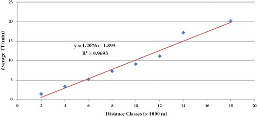
Figure 7. Nonlinear relations between the distance to the 3 nearest parks and VTTs of distance classes in five sample times (7 a.m., 9 a.m., 12 p.m., 3 p.m. and 6 p.m.) and a sharper increase of VTT in longer distances during the two peak traffic hours of 7 a.m. and 6 p.m

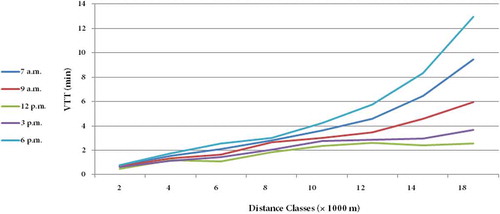
Observation of the change of VTT as a function of distance in five unique traffic conditions in Figure 7 shows interesting patterns. In light traffic conditions at 12 p.m., VTT shows a slight increase with an increase in the distance and then no change or even some slight decrease in longer distances of over 12 km. But the increase of the traffic density results in a sharper increase of VTT at longer distances leading to nonlinear increases with the distance (Figure 7). As shown in the Figures 6 and 7, both the TT and VTT show increasing trends with the increase of the distance, where, in contrast to TT which linearly increases with distance (Figure 6), VTT shows an exponential increase with the distance (Figure 7). These observations show the fact that longer distances are exposed to higher VTTs caused by traffic congestion, resulting in severe inequities in longer distances. Severe increase of VTT in longer distances, particularly during peak traffic hours, can be attributed to the increase of the diversity of access roads and traffic conditions at these distances.

The magnitude of VTT in a distance in Figure 7 is an example of traffic-related and dynamic inequity of access to urban services. Because of the increase of the traffic effects on longer traveling distances inside the urban areas, the inequity of TTs shows increasing trends in longer distances from the service centers. Therefore, considerable inequities that increase with the distance and density of traffic exist between residents with equal distances from the service centers. In contrast to the inequity of distance and ATT between residents, that are well understood and explained in previous studies, temporal dynamics of the inequity of TT and their increase with the spatial distance can be regarded as an example of the unperceived inequity. These results confirm the fact that using static indices such as the travel distance or ATT for measurement of inequity can lead to ignorance of considerable inequities.

4.5. Comparison of accessibility maps based on ATT and ITT

As shown in Figure 6, the distance and ATT during the day are linearly related. Therefore, classified maps of travel distances and ATT to parks are expected to show similar results. For a better understanding of the geographic context of the study area, the distances of each TAZ to its top-1, top-2, and top-3 closest parks are separately mapped and shown in Figure 8.

Figure 8. Distance of TAZs to their (a) top-1, (b) top-2, (c) top-3, (d) top-1 and top-2, (e) top-2 and top-3, (f) top-1 and top-3 and (g) top-1, top-2 and top-3 closest parks

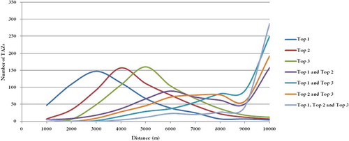
It can be seen that TAZs located in the eastern and southwestern parts of the study area is over 5 km away from their first nearest parks (Figure 8(a)) and their accessibility status is even getting worse in the second and third nearest parks (Figure 8(b-c)). Figure 8(d-f)) show the results of using two numbers of the closest parks. The result of using the three closest parks is shown in Figure 8(g). It is interesting to see how the order of selected closest parks (first, second, or third) heavily affects the accessibility of the residents (Figures 8 and 9). Distribution of parks in different distances shows normal patterns and the maximum number of the first, second, and third closest parks are respectively located in 3, 4 and 5 km from the TAZs (Figure 9). Access to two and three numbers of the closest parks requires much higher travel distances and TTs. As an example, to visit two of the three closest parks, most residents have to travel about 10 km (Figure 9). Therefore, consideration of accessibility to over one nearby park provides more useful accessibility information, not provided by considering only the one closest park.

Figure 9. Number of TAZs in different distances from their top-1, top-2, top-3, top-1 and top-2, top-1 and top-3, top-2 and top-3, top-1 and top-2 and top-3 closest parks

For visualization of the spatial effects of temporal dynamics of inequity, the gravity model as expressed in equation 1(1) ${\alpha }_i^l\left(t\right)={\sum }_{j=1}^n\left(w_j^l\times ex{p}^{\left(-t_{ij}^l\left(t\right)\right)}\right)$(1) was used to produce and compare two types of accessibility maps. One is the ATT-based accessibility index using ATTs instead of the dynamic TTs in equation 1(1) ${\alpha }_i^l\left(t\right)={\sum }_{j=1}^n\left(w_j^l\times ex{p}^{\left(-t_{ij}^l\left(t\right)\right)}\right)$(1) . This leads to the production of only one accessibility map. Another is the ITT-based accessibility maps of TAZs which use instant TTs instead of the ATT and results in the production of five temporal accessibility maps, one for each of the sample times. All the six resulting accessibility maps were classified into three classes of accessibility. These include “favorable” (TT of fewer than 8 min), “moderate” (TT of 8–20 min) and, “unfavorable” (TT of more than 20 min), respectively showing high, medium, and low accessibilities. So, the last class highlighted the deprived areas. Figures 10 and 11 highlights the distributions of the areas of unfavorable TAZs at five sample times of a working day.

Figure 10. Total area (ha) of TAZs with unfavorable accessibility (more than 20 min) to the 3-closest parks

Figure 11. Maps showing the spatial distribution of unfavorable areas (with travel times of more than 20 min) at 5 times (7 a.m., 9 a.m., 12 p.m., 3 p.m. and 6 p.m.) of a working day and a significant increase of these areas at 7 a.m. and 6 p.m., the most traffic-congested times

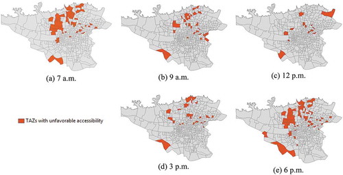
Significant impacts of traffic are evident in the variability of total areas of TAZs with unfavorable accessibilities. Such that the total areas of the unfavorable class reach their maximum of more than 10,000 ha at 6 p.m., the most traffic-congested time. This area is, considerably higher than those of the areas of unfavorable classes, 7600 ha at 7 a.m., 4607 ha at 9 a.m., 3234 ha at 12 p.m. and 4244 ha at 3 p.m.

Examination of the extracted unfavorable areas shows that “time” and “traffic” play important roles in the inequity status of accessibility of TAZs (Figure 11). An interesting result of this examination is the dynamic nature of inequity. As an example, a region may be favorable at 12 p.m. and unfavorable at 6 p.m., which is in contrast with the static accessibility approaches. This inequity can be more obvious in access to some critical service centers such as health centers or hospitals, where there is no choice of time and one has to use the service at any unexpected time. As an example, two residents may have equal fixed (time or distance) accessibilities, but they may face very unequal conditions and the chance of access in an urgent case of need for health care and hospital services. The inequity of this type can be managed by the estimation and control of the TT_max as outlined in equation 10(10) $T{T}_{\mathrm{m}\mathrm{a}\mathrm{x}}=ATT+VT{T}_{\mathrm{m}\mathrm{a}\mathrm{x}}=f\left(d\right)$(10) .

4.6. Assessment of access equity of TAZs

In order to assess the equity of accessibility of TAZs to their three closest regional parks at five times a day, the Lorenz curve was plotted for each time. Figure 12 shows the Lorenz curve where accessibility levels are compared to the residential population in each TAZ. These curves show that the lowest and highest accessibility, respectively, belong to 6 p.m. and 12 p.m., with Gini coefficients of 0.26 and 0.53 respectively. This means that if accessibility is interpreted as the number of opportunities, at peak traffic hour (at 6 p.m.), 80% of the population share only 33% of the regional park opportunities and, conversely, 20% of the remaining population share 77% of the opportunities. While at off-peak traffic hours (at 12 p.m.), 80% of the population share about 70% of the regional park opportunities, and conversely, 20% of the remaining population share 30% of the opportunities. In the same way, at other times (at 7 a.m., 9 a.m., and 3 p.m.), 70% of the population respectively share 27%, 30%, and 38% of the opportunities.

Figure 12. Lorenz curve of all population of the study area, for sample times of 7 a.m., 9 a.m., 12 p.m., 3 p.m., and 6 p.m. during a working day

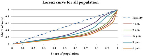
Differences in the Lorenz curves at different times of day highlight the temporal inequity of accessibility in the study area, which results from varying traffic conditions during the day. The practical effects of these inequities would depend on the demand and service type. As an example, temporal inequities and a sharp increase of VTT with distance and heavy traffic conditions would be more significant in accessing urgent demands for emergency services, hospitals, and clinics. In contrast, in the case of accessing time-limited services such as offices and schools, accessibility during the working hours can be critical.

4.7. Practical application in inequity management

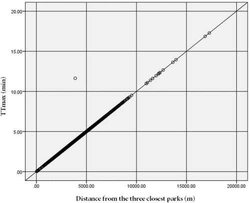
For a demonstration of the usefulness of the proposed approach for spatiotemporal inequity management, daily ATT and TT_max of each TAZ to the three closest parks were calculated, using five samples of daily TT. Investigation of the relations between the daily ATT and TT_max showed two interesting patterns (Figure 13). One pattern which is dominant and highlighted with the fitted line in Figure 13, is where ATT and TT_max show a strong linear relationship, and according to equation 10(10) $T{T}_{\mathrm{m}\mathrm{a}\mathrm{x}}=ATT+VT{T}_{\mathrm{m}\mathrm{a}\mathrm{x}}=f\left(d\right)$(10) , VTT = 0, and ATT = TT_max. This represents TAZs with minimum sensitivity to traffic conditions, which are mostly concentrated in low values of ATTs (less than 7–8 min) and negligible VTT during the working day.

Figure 13. Relations between the daily TT_max (vertical axis) and ATT (horizontal axis) for the three closest parks in the study area

Another pattern belongs to TAZs with TT_max greater than ATT (VTT > 0), which are highly exposed to traffic conditions (Figure 13). This pattern shows high variability of TT in relation to the fitted line to the first pattern which increases with the increase of ATT and TT_max.

Due to major differences of these two patterns, high temporal variability of TT in pattern 2, TAZs of this pattern are more important for spatial equity management. Because of this, two patterns have been discriminated against and separately considered. Separation of these two patterns is helpful as they display uncommon TT behaviors. These patterns are respectively, referred to as pattern 1 and pattern 2. Consideration of the relations between the TT_max (or ATT) and the distance of pattern 1 from the three closest parks shows strong linear relationships, showing the one-to-one relationships between the TT_max and distance (Figure 14). Equation of the fitted line between the TT_max (in min) and the distance, represented as d (in meters) is expressed as TT_max = ATT = 0.001d.

Figure 14. Strong linear relationship between the TT_max (vertical axis) and the distance from the three closest parks (horizontal axis) for TAZs of pattern 1 in the study area

Therefore, as an example of applying this equation, the required travel distance for TAZs of pattern 1, to access at least one of the three closest parks in less than 5 min, is less than 5 km. By applying this distance threshold for data of pattern 1, TAZs of pattern 1 are divided into two accepted and rejected classes, respectively for having less (or equal) and more than the TT_max of 5 min. Frequency of TT_max of these two classes as presented in Figures 15 and 16, which demonstrates the validity of this discrimination. As seen, maximum and minimum values of TT_max respectively in the accepted and rejected classes are equal (5 min) which is in agreement with the objectives for distance-time based discrimination of TAZs for inequity management.

Figure 15. Frequency of TT_max distribution (with maximum TT_max of 5 min) in TAZs of pattern 1, selected for having distances of less than 5 km from at least one of the three closest parks

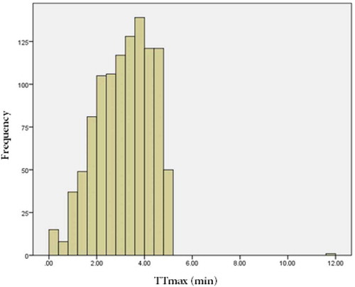
Figure 16. Frequency of TT_max distribution (with minimum TT_max of 5 min) in TAZs of pattern 1 selected for having distances of more than 5 km from the three closest parks

As control of the TT_max to lower than the desired value is the main objective in equity management projects, so TAZs of pattern 2 with an acute sensitivity to traffic conditions provide important challenges for TT equity management. Figure 17 highlights the relations between the TT_max and distance from the three closest parks for data of pattern 2. As shown, there are two minor patterns with linear relations with distance but with different slopes. However, due to the importance of controlling the maximum values of TT, the pattern with the lower slope is neglected, and the dominant pattern with higher values of TT_max, sharper slope, and stronger linear relations with the distance is selected for the line fit (Figure 17).

Figure 17. Relations between the TT_max (vertical axis) and the distance from the three closest parks (horizontal axis) for TAZs of pattern 2 in the study area

Equation of the fitted line for data of pattern 2 is TT_max = 0.003d, where the increase of the TT_max as a function of d is three times more than that of the pattern 1.

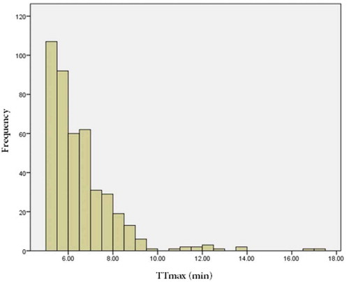
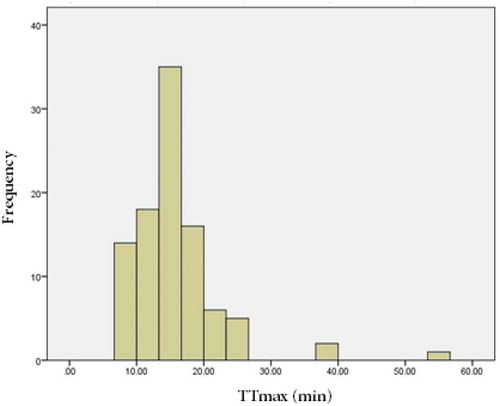
For a practical test of the validity of this equation, as an example, the required travel distances to access at least one of the three closest parks in less than 12 min are less than 4 km. By applying this distance threshold for data of pattern 2, TAZs are divided in two accepted and rejected classes respectively for having TT_max of less than (or equal to) and more than 12 min. Results of the examination of the frequency of TT_max of these two classes as presented in Figures 18 and 19 show the validity of this classification. As can be seen, the maximum and minimum values of TT_max in the two selected and rejected classes are respectively 12 and 8 min. The range of TT_max for the selected class is between 2 to 12 min, which is in perfect agreement with the objectives of having a maximum TT of fewer than 12 min. However, due to the high variability of TT_max, ignoring the second minor pattern with a gentle slope in Figure 17, and considering the maximum values of TT_max in model fitting, a number of TAZs with TT_max lower than 12 min are included in the rejected class, leading to some omission errors. The range of TT_max for this class varies between 8 to 55 min with the maximum frequency being located in 14–17 min, which is higher than the threshold value of 12 min (Figure 19). Rejected class includes 97 TAZs, from which TT_max of 17 TAZs are less than 12 min (8–12 min), which shows an accuracy of 82%. However, because of the importance of the accepted class and lack of commission errors (accepting TTs that are higher than the management aim) in this selection, the fitted model of distance-time relations can be capable of a useful tool for equity management and planning.

Figure 18. Frequency of TT_max distribution (with maximum TT_max of 12 min) in TAZs of pattern 2 selected for having distances of less than 4 km from at least one of the three closest parks

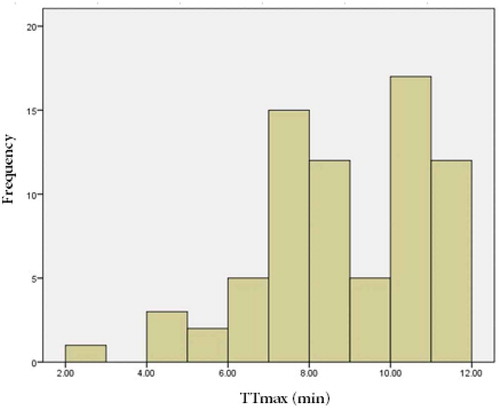
Figure 19. Frequency of TT_max distribution (with minimum TT_max of 8 min) in TAZs of pattern 2 selected for having distances of more than 4 km from the three closest parks

5. Conclusions

In this paper, the traffic-related dynamics of TTs in relation to the problem of inequity of access to the three closest urban parks in the Tehran megacity is analyzed. Traffic maps of the area at five different times of a working day are used to define TTs. Relations between the TT and the network distances from TAZs to the three closest urban parks are modeled. Results show positive relations between the TT and the distance in all five-time samples. At the same time, an increase of distance leads to an increase of the VTTs leading to different TTs of locations with similar distances to the closest service centers. The prime reason for this increase may be related to the increase of the diversity of access roads and traffic conditions in longer distances. However, the increase rate of the VTT is higher in peak traffic times (at 7 a.m. and 6 p.m. in this study). This means that TAZs within the same distance from their closest parks have to spend unequal times to access a park. Results show that the Gini coefficient of accessibility to the three closest parks shows considerable variation at different times of the day. Assuming people are interested in minimizing the required TTs to their three closest parks, then they have to choose different times, and there will be inequities between residents in their best times to visit parks. Those areas with low distance, low TTs, and low VTTs to a park would have more temporal opportunities to visit a park, whereas residents with higher TTs and VTTs for a park would have limited temporal opportunities to visit parks. As an example, the results of this study show that the best and worst times to visit parks in the study area coincide with the traffic conditions and respectively include 12 p.m. (low traffic time) and 6 p.m. (high traffic congestion time). Although inequities of time choice may be less important with a visit to a park, it would be more important in other cases where time choice is limited. An example is when one has to attend school at a certain time or when there is an urgent and instant need for the services of a health center or a hospital.

Because of the focus of this research on the examination of traffic-related TTs and distance relationships, access to parks has been based on driving either by private or public cars. Although this may not be valid for areas located in closer distances to parks because of the irregular distribution of parks, and high variation of access distances (in some areas up to 18 km), traveling to parks by driving is a normal practice in the study area. In addition, driving by car is the only access choice for children, elderlies, and people with disabilities. In reality, a combination of different transportation modes is used, and traffic plays a more important role in longer distances. This is in agreement with the findings of this research that longer distances coincide with higher values of VTT, where travel by car is the preferred transportation type. Samples of traffic conditions have been limited to five times in a few working days, which may not well represent the dynamics of traffic conditions. In this research, TTs and VTTs in three routes from each TAZ to the 3 closest service centers, defined by the minimum network distance concept, are studied. In practice, a collection of alternative routes from each TAZ to a given service center may be considered, and the one with the minimum TT will be preferred. Due to the complexities of considering variable routes from each place to a given destination and the resulting spatial inequities, a single shortest route for each origin and destination is used in this research. However, for the reduction of the limitations caused by considering only a single route and destination, three routes and destinations for each TAZ are used and the temporal dynamics of their TTs are evaluated. Although consideration of alternative routes for minimizing the TTs may lead to a reduction of the VTTs and compensation of some highlighted inequities in this research, this does not undermine the important role of time and distance relations in the variability of access inequities. Evaluation of temporal dynamics of spatial inequalities under variable routes and traffic conditions is an important problem, which is the subject of our continuing research.

Method and concepts of distance and traffic-related inequities of accessibility developed in this research can be adopted for inequity studies in other geographic areas and public service centers. The education and health-related centers in particular, have temporal inequities in accessibility that can lead to major discriminations and impacts among residents. Assessment of relations between the temporal and distance-based inequity of accessibility to urban services reveals new knowledge and information which can be useful for more precise and realistic spatial equity assessment and more effective spatial planning. Results indicated a significant relationship between the distance, TT and VTT. These relations can help urban planners to reconsider the traffic congestion impacts on access equity in their decisions and planning. In a way that, by defining the relationship between the access distance, TT, and VTT at different times of the day, urban planners can analyze and manage both the spatial and temporal inequity problems. As an example, an examination of the inequity of travel time in the Tehran megacity shows that maximum TTs from TAZs to the closest parks show high variability ranging from 1 to about 55 min. By using the developed linear model between the TT_max and distance, to decrease the maximum TT of TAZs to their closest park to less than 12 min, the maximum distance of TAZs to the closest parks should be less than 4 km. These results can be used to map and identify the deprived TAZs as well as to highlight the prime priority areas for the establishment of new parks.

In ideal situations of equity, equal TTs with zero variations may be assumed. But in practice, inequity is part of the real-life, and its minimization or control using existing standards is the key objective. Therefore, minimizing differences of TTs and their variations provides a more realistic model for the management of the inequity. Strong relations observed between the distance, TTs and VTTs show how inequity of distance leads to temporal inequities, how spatial inequity plays a key role in the management of inequity, and finally how temporal inequity can be controlled by reducing the spatial inequities. As an example, statistical models of interactions between the distance, TT, and VTT as developed in this research can be used to define the maximum acceptable accessibility distances to different service centers in varying geographic regions. Such that inequities of TTs between residents in different or equal distances from the closest service centers are reduced to a standard or maximum acceptable level.

Data availability statement

The data that support the findings of this study were derived from the following resources available in the public domains: “https://map.tehran.ir/”; “https://www.google.com/maps/@35.7138432,51.3396774,12z” and “https://www.amar.org.ir”. These data are also available from the corresponding author, Alimohammadi, A. upon reasonable request.

Additional information

Notes on contributors

Tahereh Ghaemi Rad

Tahereh Ghaemi Rad is a PhD candidate in GIS Dept. of Faculty of Geomatics Engineering. She received the Master degree from the Center of Excellence in Geospatial Information Technology, K.N.Toosi University of Technology. Her research interests are spatial/social equity analysis and smart city problems.

Abbas Alimohammadi

Abbas Alimohammadi is a professor in GIS Dept. and Center of Excellence in Geospatial Information Technology of the Faculty of Geomatics Engineering, K. N. Toosi University of Technology. He received the PhD degree from the Australian National University. His research interests are GIS/spatial analysis in urban and environmental problems, spatial data science and spatial optimization.

References

- Arranz-López, A., J. A. Soria-Lara, and P.-C. Ángel. 2019. “Social and Spatial Equity Effects of non-Motorised Accessibility to Retail.” Cities 86: 71–82. doi:https://doi.org/10.1016/j.cities.2018.12.012.
- Artmann, M., C. Mueller, L. Goetzlich, and A. Hof. 2019. “Supply and Demand Concerning Urban Green Spaces for Recreation by Elderlies Living in Care Facilities: The Role of Accessibility in an Explorative Case Study in Austria.” Frontiers in Environmental Science 7: 136. doi:https://doi.org/10.3389/fenvs.2019.00136.
- Berke, P., and M. Manta. 1999. “Planning for Sustainable Development: Measuring Progress in Plans.” Cambridge, MA: Lincoln Institute of Land Policy.
- Bhat, C., S. Handy, K. Kockelman, H. Mahmassani, A. Gopal, I. Srour, and L. Weston. 2002. “ Development of an Urban Accessibility Index: Formulations, Aggregation, and Application.” Center for Transportation Research, the University of Texas at Austin. Project 7-4938.
- Brown, M. C. 1994. “Using Gini-style Indices to Evaluate the Spatial Patterns of Health Practitioners: Theoretical Considerations and an Application Based on Alberta Data.” Social Science & Medicine 38 (9): 1243–1256. doi:https://doi.org/10.1016/0277-9536(94)90189-9.
- Chang, H.-S., and C.-H. Liao. 2011. “Exploring an Integrated Method for Measuring the Relative Spatial Equity in Public Facilities in the Context of Urban Parks.” Cities 28 (5): 361–371. doi:https://doi.org/10.1016/j.cities.2011.04.002.
- Cheng, G., X. Zeng, L. Duan, L. Xiaoping, H. Sun, T. Jiang, and L. Yuli. 2016. “Spatial Difference Analysis for Accessibility to High Level Hospitals Based on Travel Time in Shenzhen, China.” Habitat International 53: 485–494. doi:https://doi.org/10.1016/j.habitatint.2015.12.023.
- Choi, H. S., and K. H. Ahn. 2013. “Assessing the Sustenance and Evolution of Social and Cultural Contexts within Sustainable Urban Development, Using as a Case the MAC in South Korea.” Sustainable Cities and Society 6: 51–56. doi:https://doi.org/10.1016/j.scs.2012.08.003.
- Dadashpoor, H., and F. Rostami. 2017. “Measuring Spatial Proportionality between Service Availability, Accessibility and Mobility: Empirical Evidence Using Spatial Equity Approach in Iran.” Journal of Transport Geography 65: 44–55. doi:https://doi.org/10.1016/j.jtrangeo.2017.10.002.
- Din, E., H. Serag, A. Shalaby, H. E. Farouh, and S. A. Elariane. 2013. “Principles of Urban Quality of Life for a Neighborhood.” HBRC Journal 9 (1): 86–92. doi:https://doi.org/10.1016/j.hbrcj.2013.02.007.
- Fotini, M. 2017. “A New Anthropocentric Approach in Accessibility Analysis: The Activity Space and the Accessibility Measures.” Transportation Research Procedia 24: 491–498. doi:https://doi.org/10.1016/j.trpro.2017.05.088.
- García-Albertos, P., M. Picornell, M. H. Salas-Olmedo, and J. Gutiérrez. 2019. “Exploring the Potential of Mobile Phone Records and Online Route Planners for Dynamic Accessibility Analysis.” Transportation Research Part A: Policy and Practice 125: 294–307.
- Guzman, L. A., D. Oviedo, and C. Rivera. 2017. “Assessing Equity in Transport Accessibility to Work and Study: The Bogotá Region.” Journal of Transport Geography 58: 236–246. doi:https://doi.org/10.1016/j.jtrangeo.2016.12.016.
- Hu, W., J. Tan, L. Mengya, J. Wang, and F. Wang. 2018. “Impact of Traffic on the Spatiotemporal Variations of Spatial Accessibility of Emergency Medical Services in Inner-City Shanghai.” Environment and Planning B: Urban Analytics and City Science 47 (5): 841–854
- Kimpton, A. 2017. “A Spatial Analytic Approach for Classifying Greenspace and Comparing Greenspace Social Equity.” Applied Geography 82: 129–142. doi:https://doi.org/10.1016/j.apgeog.2017.03.016.
- Kompil, M., C. Jacobs-Crisioni, L. Dijkstra, and C. Lavalle. 2019. “Mapping Accessibility to Generic Services in Europe: A Market-Potential Based Approach.” Sustainable Cities and Society 47: 101372. doi:https://doi.org/10.1016/j.scs.2018.11.047.
- Lawal, O., and F. E. Anyiam. 2019. “Modelling Geographic Accessibility to Primary Health Care Facilities: Combining Open Data and Geospatial Analysis.” Geo-Spatial Information Science 22 (3): 174–184. doi:https://doi.org/10.1080/10095020.2019.1645508.
- Liao, C.-H., C. Hsueh-Sheng, and K.-W. Tsou. 2009. “Explore the Spatial Equity of Urban Public Facility Allocation Based on Sustainable Development Viewpoint.” In Preceedings REAL CORP 2009, Tagungsband, edited by Manfred Schrenk, Vasily V. Popovich, Dirk Engelke and Pietro Elisei, 22-25 April 2009, 137–145.
- Lotfi, S., and M. J. Koohsari. 2009. “Measuring Objective Accessibility to Neighborhood Facilities in the City (A Case Study: Zone 6 in Tehran, Iran).” Cities 26 (3): 133–140. doi:https://doi.org/10.1016/j.cities.2009.02.006.
- Lucas, K., B. van Wee, and K. Maat. 2016. “A Method to Evaluate Equitable Accessibility: Combining Ethical Theories and Accessibility-based Approaches.” Transportation 43 (3): 473–490. doi:https://doi.org/10.1007/s11116-015-9585-2.
- Lucy, W. 1981. “Equity and Planning for Local Services.” Journal of the American Planning Association 47 (4): 447–457. doi:https://doi.org/10.1080/01944368108976526.
- Makri, M.-C., and C. Folkesson. 1999. Accessibility Measures for Analyses of Land-use and Travelling with Geographical Information Systems. Department of Technology and Society, Lund Institute of Technology, Lund University & Department of Spatial Planning, University of Karlskrona/Ronneby, Sweden.
- Mansour, S. 2016. “Spatial Analysis of Public Health Facilities in Riyadh Governorate, Saudi Arabia: A GIS-based Study to Assess Geographic Variations of Service Provision and Accessibility.” Geo-spatial Information Science 19 (1): 26–38. doi:https://doi.org/10.1080/10095020.2016.1151205.
- Neutens, T., T. Schwanen, F. Witlox, and P. De Maeyer. 2010. “Equity of Urban Srvice Delivery: A Comparison of Different Accessibility Measures.” Environment and Planning A 42 (7): 1613–1635. doi:https://doi.org/10.1068/a4230.
- Nichols, S. 2001. “Measuring the Accessibility and Equity of Public Parks: A Case Study Using GIS.” Managing Leisure 6 (4): 201–219. doi:https://doi.org/10.1080/13606710110084651.
- Oh, K., and S. Jeong. 2007. “Assessing the Spatial Distribution of Urban Parks Using GIS.” Landscape and Urban Planning 82 (1): 25–32. doi:https://doi.org/10.1016/j.landurbplan.2007.01.014.
- Omer, I. 2006. “Evaluating Accessibility Using House-Level Data: A Spatial Equity Perspective.” Computers, Environment and Urban Systems 30 (3): 254–274. doi:https://doi.org/10.1016/j.compenvurbsys.2005.06.004.
- Pasaogullari, N., and N. Doratli. 2004. “Measuring Accessibility and Utilization of Public Spaces in Famagusta.” Cities 21 (3): 225–232. doi:https://doi.org/10.1016/j.cities.2004.03.003.
- Salonen, M. 2014. “Analysing Spatial Accessibility Patterns with Travel Time and Distance Measures: Novel Approaches for Rural and Urban Contexts.” PhD diss., University of Helsinki.
- Shirmohammadli, A., C. Louen, and V. Dirk. 2016. “Exploring Mobility Equity in A Society Undergoing Changes in Travel Behavior: A Case Study of Aachen, Germany.” Transport Policy 46: 32–39. doi:https://doi.org/10.1016/j.tranpol.2015.11.006.
- Stępniak, M., and S. Goliszek. 2017. “Spatio-Temporal Variation of Accessibility by Public Transport—The Equity Perspective.” In The Rise of Big Spatial Data, edited by I. Ivan, A. Singleton, J. Horák and I Inspektor, 241–261. Cham: Springer.
- Tahmasbi, B., M. H. Mansourianfar, H. Haghshenas, and I. Kim. 2019. “Multimodal Accessibility-Based Equity Assessment of Urban Public Facilities Distribution.” Sustainable Cities and Society 49: 101633. doi:https://doi.org/10.1016/j.scs.2019.101633.
- Taleai, M., R. Sliuzas, and J. Flacke. 2014. “An Integrated Framework to Evaluate the Equity of Urban Public Facilities Using Spatial Multi-Criteria Analysis.” Cities 40: 56–69. doi:https://doi.org/10.1016/j.cities.2014.04.006.
- Talen, E. 1997. “The Social Equity of Urban Service Distribution: An Exploration of Park Access in Pueblo, Colorado, and Macon, Georgia.” Urban Geography 18 (6): 521–541. doi:https://doi.org/10.2747/0272-3638.18.6.521.
- Talen, E., and L. Anselin. 1998. “Assessing Spatial Equity: An Evaluation of Measures of Accessibility to Public Playgrounds.” Environment and Planning A 30 (4): 595–613. doi:https://doi.org/10.1068/a300595.
- Tsou, K.-W., Y.-T. Hung, and Y.-L. Chang. 2005. “An Accessibility-Based Integrated Measure of Relative Spatial Equity in Urban Public Facilities.” Cities 22 (6): 424–435. doi:https://doi.org/10.1016/j.cities.2005.07.004.
- Van Wee, B. 2016. “Accessible Accessibility Research Challenges.” Journal of Transport Geography 51: 9–16. doi:https://doi.org/10.1016/j.jtrangeo.2015.10.018.
- Van Wee, B., and K. Geurs. 2011. “Discussing Equity and Social Exclusion in Accessibility Evaluations.” European Journal of Transport and Infrastructure Research 11: 4.
- Welch, T. F., and S. Mishra. 2013. “A Measure of Equity for Public Transit Connectivity.” Journal of Transport Geography 33: 29–41. doi:https://doi.org/10.1016/j.jtrangeo.2013.09.007.
- Wen, H., Y. Xiao, C. M. H. Eddie, and L. Zhang. 2018. “Education Quality, Accessibility, and Housing Price: Does Spatial Heterogeneity Exist in Education Capitalization?” Habitat International 78: 68–82. doi:https://doi.org/10.1016/j.habitatint.2018.05.012.
- Wu, C., Y. Xinyue, Q. Du, and P. Luo. 2017. “Spatial Effects of Accessibility to Parks on Housing Prices in Shenzhen, China.” Habitat International 63: 45–54. doi:https://doi.org/10.1016/j.habitatint.2017.03.010.
- Xu, C., D. Haase, D. O. Pribadi, and S. Pauleit. 2018. “Spatial Variation of Green Space Equity and Its Relation with Urban Dynamics: A Case Study in the Region of Munich.” Ecological Indicators 93: 512–523. doi:https://doi.org/10.1016/j.ecolind.2018.05.024.
- Ye, Z., and H. Xiang. 2015. “Research on the Basic Education Spatial Distribution in Shandong Province” Paper presented at the 23rd International Conference on Geo-Informatics, IEEE, Wuhan, China.
- Zhang, F., L. Dezhi, S. Ahrentzen, and J. Zhang. 2019. “Assessing Spatial Disparities of Accessibility to Community-Based Service Resources for Chinese Older Adults Based on Travel Behavior: A City-Wide Study of Nanjing, China.” Habitat International 88: 101984. doi:https://doi.org/10.1016/j.habitatint.2019.05.003.
- Zhang, X., L. Hua, and J. B. Holt. 2011. “Modeling Spatial Accessibility to Parks: A National Study.” International Journal of Health Geographics 10 (1): 31. doi:https://doi.org/10.1186/1476-072X-10-31.
- Zheng, Z., H. Xia, S. Ambinakudige, Y. Qin, L. Yang, Z. Xie, L. Zhang, and G. Haibin. 2019. “Spatial Accessibility to Hospitals Based on Web Mapping API: An Empirical Study in Kaifeng, China.” Sustainability 11 (4): 1160. doi:https://doi.org/10.3390/su11041160.