LEO satellite clock analysis and prediction for positioning applications

ABSTRACT

The positioning service aided by low Earth orbit (LEO) mega-constellations has become a hot topic in recent years. To achieve precise positioning, accuracy of the LEO clocks is important for single-receiver users. To bridge the gap between the applicable time of the clock products and the time of positioning, the precise LEO clocks need to be predicted over a certain period depending on the sampling interval of the clock products. This study discusses the prediction errors for periods from 10 s to 1 h for two typical LEO clock types, i.e. the ultra-stable oscillator (USO) and the oven-controlled crystal oscillator (OCXO). The prediction is based on GNSS-determined precise clock estimates, where the clock stability is related to the GNSS estimation errors, the behaviors of the oscillators themselves, the systematic effects related to the environment and the relativistic effects, and the stability of the time reference. Based on real data analysis, LEO clocks of the two different types are simulated under different conditions, and a prediction model considering the systematic effects is proposed. Compared to a simple polynomial fitting model usually applied, the proposed model can significantly reduce the prediction errors, i.e. by about 40%-70% in simulations and about 5%-30% for real data containing different miss-modeled effects. For both clock types, short-term prediction of 1 min would result in a root mean square error (RMSE) of a few centimeters when using a very stable time reference. The RMSE amounts to about 0.1 m, when a typical real-time time reference of the national center for space studies (CNES) real-time clocks was used. For long-term prediction of 1 h, the RMSE could range from below 1 m to a few meters for the USOs, depending on the complexity of the miss-modeled effects. For OCXOs, the 1 h prediction could lead to larger errors with an RMSE of about 10 m.

KEYWORDS:

• LEO
• clock prediction
• USO
• OCXO
• relativistic effects

1. Introduction

In recent years, thousands of low Earth orbit (LEO) satellites launched or planned to be launched by companies like SpaceX, OneWeb, Iridium and Orbcomm are about to form a dense satellite network near the Earth, i.e. with an altitude from a few hundreds of kilometers to about 1500 km (Montenbruck and Gill 2000; Reid et al. 2018). Considering the large number of the LEO satellites and their strong signal strength, the LEO mega-constellations have been considered for positioning purpose to assist the current global navigation satellite systems (GNSSs), in particular in challenging environments, using either signals generated by additional navigation payload, or the signals of opportunity (Coluccia, Ricciato, and Ricci 2014). The addition of the LEO satellites in positioning does not only reduce the position dilution of precision (PDOP) (Han et al. 2020; Wang, Teunissen, and El-Mowafy 2020), especially in areas with limited GNSS satellite visibility, but also enables positioning in deep attenuation environments, including indoors (Lawrence et al. 2017). The rapidly changing LEO satellite geometry, as shown in (Ge et al. 2018; Li et al. 2018), also greatly reduces the precise point positioning (PPP) convergence time.

The accuracy of the satellite orbits and clocks is important for the positioning service on the ground. For real-time positioning, the orbits and clocks need to be predicted over a short- or long-period, with the corresponding model parameters delivered to users with either a low or a high sampling rate. Diverse studies have been performed for LEO orbit prediction in different forms, using different models and for different prediction periods (Reid et al. 2018; Ge et al. 2020; Wang and El-Mowafy 2020). In addition to the orbits, the clocks also directly influence the user range error (URE), and thus the positioning accuracy. As the GNSS receiver and the signal transmitter on-board the LEO satellite can be synchronized with the same frequency oscillator (Wang et al. 2018), it is possible to determine the clock offsets together with the reduced-dynamic orbits using GNSS observations, which can normally reach an accuracy of centimeters when good dynamic models and high-precision GNSS products are used (Li et al. 2017). It was reported that hardware biases could exist between the receiving and the transmitting time, and a perfect calibration remains a challenge. In (Wang et al. 2018), the hardware bias was assumed as a constant, and in (Yang et al. 2020), a different strategy using a network of ground tracking stations was applied when estimating the LEO clocks.

Similar to the orbital products, high-precision clock estimation is not enough for real-time positioning users. The LEO clocks need to be predicted into the near future to bridge the gap between the applicable time of the clock products and the positioning time. Many studies have been performed for GNSS clock prediction. Polynomial models were used for the International GNSS Service (IGS) (Johnston, Riddell, and Hausler 2017) real-time service (RTS) clock prediction in the short-term of a few minutes (Hadas and Bosy 2015) and for the broadcast clocks in the navigation message in the long-term of up to a few hours (Romero 2020). Cyclic terms were added to compensate for the remaining periodic effects (Heo, Cho, and Heo 2010; El-Mowafy, Deo, and Kubo 2017), having time-adaptive weighting functions applied (Huang, Zhang, and Xu 2014), or having periodic parameters obtained through fast Fourier transform (FFT) (Lv et al. 2020). Moreover, a wavelet neural network model was employed on single-differenced clocks between subsequent epochs to deal with influences of external factors (Wang et al. 2016). Modified grey model (Zheng, Lu, and Chen 2008) and autoregressive integrated moving average model (Zhou et al. 2016) were also employed to improve the prediction of the GNSS clocks (Zhou et al. 2016). Compared to the GNSS clocks, the LEO satellite clock behaviors were less investigated. The different clock types on LEO satellites and their noise behaviors would lead to different error patterns in the prediction. Meanwhile, LEO satellites experience different systematic effects caused by, e.g. the space measurement environment and the more complicated relativistic effects. The stability of the reference time-scale in real-time also needs to be considered in the LEO clock prediction, as their influences on the predicted clocks could be different due to the different prediction periods of diverse LEO satellites, as well as those of the GNSS satellites. Note that this paper includes the epochs with jumps in the real-time time references, but provides both the results considering and ignoring the influences of the reference time-scale.

In general, the prediction of the LEO clocks is influenced by the following factors:

• The prediction interval used;

• Stability of the frequency oscillator;

• GNSS estimation errors caused by, e.g. noise, multipath and errors in the real-time GNSS products;

• Systematic effects caused by the space measurement environment, the relativistic effects or other sources;

• Stability of the time reference.

Among the five factors listed above, some are highly related to the employed processing strategy, models and resources. Some of them, e.g. the oscillator stability, cannot be changed through data processing. Luckily, nowadays very stable frequency oscillators like the ultra-stable oscillators (USO) are used in diverse space missions that require good short-term clock stability, e.g. for applications like radio occultation (Griggs, Kursinski, and Akos 2015). Examples are missions like the gravity recovery and climate experiment (GRACE) (Case, Kruizinga, and Wu 2010), the GRACE Follow-On (GRACE-FO) (Wen et al. 2019), and the SENTINEL-3 (ESA 2012). The short-term stability of a typical USO can reach the level of ${10}^{-13}$ (Dunn et al. 2003; Ko and Tapley 2010; Bertiger et al. 2003; Weinbach and Schön 2012). Without a very high requirement on clock stability, most LEO satellites are equipped with oven-controlled crystal oscillators (OCXOs), or more practically, the temperature-compensated crystal oscillators (TCXOs), which have a lower stability (Et Alia 2019). As shown in (Hudson et al. 2019; Defraigne 2017), good OCXOs can also reach a short-term stability of ${10}^{-12}$. The good stabilities of these frequency oscillators on-board LEO satellites have offered the possibility of short-term clock prediction with acceptable tolerance.

In addition to the clock quality, the systematic effects remaining in the LEO satellite clocks also need to be considered during the prediction of the clock. The once-per-revolution (1/rev) and twice-per-revolution (2/rev) periodic behaviors are known to be related to the relativistic effects in the LEO clocks. As the LEO satellites are much nearer to the Earth compared to the GNSS satellites, the $J_2$ effects caused by the Earth’s oblateness need to be considered. A perfect correction of these effects, however, is challenging (Larson et al. 2007). Other factors like voltage variations could also be linked to the 1/rev effects. Apart from the systematic effects related to the LEO satellite periods, large long- and mid-term periodic effects are also observable in, e.g. the GRACE-FO satellite clocks, which are suspected to be related to the temperature variations on-board. Last, but not least, for real-time positioning, the LEO clock estimates are referred to the time reference of the real-time GNSS clock products. This real-time time reference, however, might not always be as stable as those used in the final GNSS products. All these effects could significantly influence clock prediction. In this study, the time-related prediction errors of LEO satellite clocks are depicted under different conditions, for different clock types, and applying different models. Note that the accuracy requirement of the LEO clock prediction is highly related to the type of positioning application itself.

The paper starts with a proposed infrastructure for generating and broadcasting the LEO clock parameters. The LEO satellite clocks are then simulated for high-quality USOs and OCXOs, where the GNSS estimation errors, the LEO oscillator stability, the systematic effects and the influences of the time references are considered and discussed. Next, a prediction model is proposed and compared with the simple polynomial fitting model with respect to the prediction errors from 10 s to 1 h to check their feasibility for both high-sampled and low-sampled clock products. Subsequently, degradations caused by different miss-modeled effects of real data are discussed. Conclusions and discussions are given in the end.

2. LEO clock products

Making use of the GNSS observations collected on-board LEO satellites, the high-accuracy LEO clocks can be estimated together with the LEO orbits. As one of the two approaches to be discussed in this study (see Figure 1), the GNSS observations are supposed to be collected by the LEO satellites and then transmitted to the ground monitoring stations (GMSs) (see the red arrows). The GMSs should form a network with a specific density and distribution, which considers the orbital characteristics of the LEO satellites and the time gaps allowed between subsequent signal transmissions (Wang and El-Mowafy 2020). The master processing center (MPC) then collects the GNSS data from multiple GMSs via Internet links as soon as they are available (see the white arrows), and performs then the reduced-dynamic precise orbit determination (POD) using comprehensive dynamic models. With the precise clock estimates, the corresponding clock parameters used for the prediction are then produced and transmitted to users via the Internet (see the yellow arrow). The users make use of these clock parameters to predict the LEO clocks into the near future, for their implementation in positioning using LEO signals, before the next set of the clock parameters are available.

Figure 1. Signal pathway for delivering the LEO clock products. Note that the locations of the ground monitoring stations (GMSs), the master processing center (MPC) and the users are only given as examples for purpose of illustration.

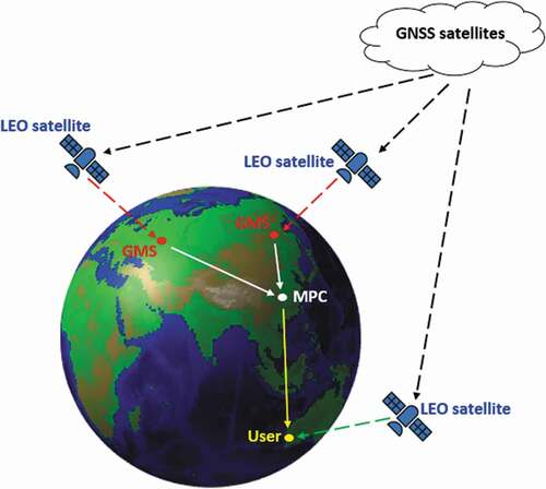
For short prediction periods, a dense network of GMSs is required to guarantee the continuous visibility of LEO satellites. As an alternative approach, the LEO clocks can also be processed in real-time on-board the satellite, so that the clock parameters can be directly broadcast to users through a satellite link (see the green arrow in Figure 1). As limitations, for applications requiring high-accuracy clock products, e.g. PPP, real-time high-precision GNSS products need to be used on-board instead of the GNSS broadcast ephemeris and clocks. Some commercial services, e.g. the Fugro G4 service, have nowadays offered this choice by broadcasting high-precision GNSS orbits and clocks in real-time through the geostationary Earth orbit (GEO) link (Hauschild et al. 2016). In addition, although only having a regional service area, the Japanese Quasi-Zenith Satellite System (QZSS) satellites broadcast high-precision GNSS products through the Centimeter Level Augmentation Service (CLAS) and the Multi-GNSS Advanced Demonstration of Orbit and Clock Analysis (MADOCA) service (Zhang et al. 2019). The second-generation Australia/New Zealand Satellite-Based Augmentation System (SBAS) has also enabled SBAS-aided PPP service by broadcasting high-precision GPS and Galileo products over the Asia-Pacific region (El-Mowafy, Cheung, and Rubinov 2020). Such service extension to a global coverage is expected in the future. Apart from the real-time high-precision GNSS products, another limitation for the on-board processing can be attributed in some satellites to the limited computational power, which leads to the usage of simplified dynamic models in the POD and thus reduced precision in both the orbits and the clocks (Montenbruck and Ramos-Bosch 2008). Considering this fact, in this contribution, the clock estimates are thus also estimated with the kinematic POD without using any dynamic models.

In this study, as an example, the POD and the clock estimation are performed using the ionosphere-free (IF) combination of the GPS code and phase observations on L1 and L2 with:

(1) $\mathrm{E}(\mathrm{\Delta }{\phi }_{IF})=A\mathrm{\Delta }r+c\times \mathrm{\Delta }\tilde{t}+{\lambda }_{IF}\times {\tilde{N}}_{IF}$(1)

(2) $\mathrm{E}\left(\mathrm{\Delta }{p}_{IF}\right)=A\mathrm{\Delta }r+c\times \mathrm{\Delta }\tilde{t}$(2)

with

(3) $\mathrm{\Delta }\tilde{t}=\mathrm{\Delta }t+d_{L,IF}/c$(3)

(4) ${\lambda }_{IF}=\frac{c}{f_1+f_2}$(4)

(5) ${\tilde{N}}_{IF}=\frac{f_1^2{\lambda }_1{N}_1-f_2^2{\lambda }_2{N}_2}{c\left(f_1-f_2\right)}+\frac{{\xi }_{L,IF}-{\xi }_{IF}^G-d_{L,IF}+d_{IF}^G}{{\lambda }_{IF}}$(5)

where the IF phase and code observed-minus-computed (O-C) terms are represented by $\mathrm{\Delta }{\phi }_{IF}$ and $\mathrm{\Delta }{p}_{IF}$, respectively. $\mathrm{E}\left(\cdot \right)$ is the expectation operator. $c$ denotes the speed of light, and $f_j$, ${\lambda }_j$ and $N_j$ ($j$=1, 2) denote the frequency, the wavelength, and the integer ambiguity vector on frequency $j$, respectively. The estimable LEO clock $\mathrm{\Delta }\tilde{t}$ contains the clock offset $\mathrm{\Delta }t$ and the IF combination of the LEO satellite code bias on L1 and L2 $d_{L,IF}$. The float estimable ambiguity vector ${\tilde{N}}_{IF}$ contains, in addition to the ambiguity terms, the IF combination of the LEO satellite phase and code biases $({\xi }_{L,IF}$, $d_{L,IF})$ and the GPS satellite phase and code bias vectors $({\xi }_{IF}^G$, $d_{IF}^G$), which are all assumed to be constant during the daily arc processing. Note that the precise GPS clocks are assumed to contain the IF combination of the GPS satellite code biases ($d_{IF}^G$), which are corrected in the O-C terms. The estimable LEO satellite clocks $\mathrm{\Delta }\tilde{t}$ are estimated in a least-squares adjustment as epoch-wise parameters without any temporal constraints, and ${\tilde{N}}_{IF}$ are assumed to be constant before a cycle slip is detected.

The estimable orbital elements $\mathrm{\Delta }r$ (based on an a priori orbit processed with simpler dynamic models) and its design matrix $A$ differs for the kinematic ($\mathrm{\Delta }{r}_K,A_K$) and the reduced-dynamic ($\mathrm{\Delta }{r}_{RD},A_{RD}$) modes with:

(6) $A_K={\left[u^1,\cdots ,u^m\right]}^T$(6)

(7) $\mathrm{\Delta }{r}_K={\left[\mathrm{\Delta }{r}_x,\mathrm{\Delta }{r}_y,\mathrm{\Delta }{r}_z\right]}^T$(7)

(8) $A_{RD}=\left[A_0,A_D,A_S\right]$(8)

(9) $\mathrm{\Delta }{r}_{RD}={\left[\mathrm{\Delta }{K}_0,\mathrm{\Delta }{P}_D,P_S\right]}^T$(9)

where $u^s$ ($s=1,\cdots ,m$) represents 3-dimensional (3D) unit vector from the GPS satellite $s$ to the LEO satellite, with $m$ denoting the number of the GPS satellites. $\mathrm{\Delta }{r}_x$, $\mathrm{\Delta }{r}_y$ and $\mathrm{\Delta }{r}_z$ denote the LEO satellite position increments in the X-, Y-, Z-directions within, e.g. IGS14. For the reduced-dynamic mode, the six Keplerian elements $\mathrm{\Delta }{K}_0$ (Dach et al. 2015), the dynamic parameters $\mathrm{\Delta }{P}_D$, as well as the stochastic accelerations $P_S$ in pre-defined time intervals are estimated. $\mathrm{\Delta }{P}_D$ and $P_S$ are used to account for the perturbation accelerations that are not contained in the existing dynamic models (see Table 1), e.g. air drag and solar radiation pressure. The term $\mathrm{\Delta }{P}_D$ consists of accelerations in constant ($\mathrm{\Delta }{a}_o$) and periodic terms ($\mathrm{\Delta }{a}_c,\mathrm{\Delta }{a}_s$), so that the corresponding acceleration $\mathrm{\Delta }{a}_D$ can be calculated with:

(10) $\mathrm{\Delta }{a}_D=\mathrm{\Delta }{a}_0+\mathrm{\Delta }{a}_{c}cos\left(U\right)+\mathrm{\Delta }{a}_s\mathrm{s}\mathrm{i}\mathrm{n}\left(U\right)$(10)

Table 1. Processing details of the POD and clock estimation. PCO and PCV are the phase center offset and variation, respectively. IERS is an abbreviation for the International Earth Rotation and Reference Systems Service

Parameters	Description
Sampling interval	10 s
Elevation cutoff angle	5 degrees
Measurements	IF combination of GPS phase (L1, L2) and code (P1, P2)
Estimation interval	24 h
Existing dynamic models (for reduced-dynamic mode)	Gravity of the Earth: EGM2008, degree 120 (Pavlis et al. 2008) Gravity of other planets: JPL DE405 (Planetary ephemeris) (Standish 1998) Tides of solid Earth and Pole: IERS Conventions 2010 (Petit and Luzum 2010) Ocean tides: FES2004 (Lyard et al. 2006) Relativistic effects
Corrections in the O-C terms	GNSS/LEO antenna offsets, PCOs, PCVs Geometric distance between the a p riori LEO orbits and the GPS orbits GPS satellite clocks and the a priori LEO satellite clocks Phase wind-up effects Relativistic effects in the GPS clocks Shapiro relativistic corrections between LEO and GPS satellites

where $U$ represents the LEO satellite’s argument of latitude. Here only the constant terms $\mathrm{\Delta }{a}_0$ were estimated to avoid over-parameterization with the stochastic accelerations. The stochastic accelerations were estimated within 6 min intervals, and are constrained to zeros with a standard deviation of $5\times {10}^{-9}$ $\mathrm{m}/{\mathrm{s}}^2$ in this study. The design matrices $A_0$, $A_D$ and $A_S$ correspond to the partial derivatives of the observations with respect to $\mathrm{\Delta }{K}_0$, $\mathrm{\Delta }{P}_D$ and $P_S$, respectively. The 3D LEO orbital positions can then be computed using the estimated elements in $\mathrm{\Delta }{r}_{RD}$ with numerical integration. The details of the processing method are given in Table 1.

As shown in Equation (3)(3) $\mathrm{\Delta }\tilde{t}=\mathrm{\Delta }t+d_{L,IF}/c$(3) , the expectation of the estimated LEO satellite clock $\mathrm{\Delta }\tilde{t}$ contains also the IF combination of the LEO satellite code biases. The LEO satellite clock to be transmitted to the ground is then further biased by the hardware delay between the receiving and transmitting time (Section 1). Both biases are assumed to be constant in this study (Wang et al. 2018), and thus do not influence the clock prediction.

3. LEO clocks in the simulations

In this section, the LEO clock estimates, which are referred to the time reference of the real-time GPS clocks used in the estimation, are simulated. The clock simulation considers the GNSS estimations errors, the LEO oscillator stability, the additional systematic effects and the stability of the time reference. It will be discussed in the next four sub-sections.

3.1. GNSS estimation errors

Based on the processing procedures introduced in Section 2, the GNSS estimation errors of the LEO satellite clocks are evaluated in both the reduced-dynamic and kinematic modes. In general, the factors influencing the LEO clock estimation errors can be summarized as follows:

• Observation noise and multipath

• Accuracy of the real-time GNSS orbits and clocks

• Model deficiencies in the LEO orbit

• Observation model, i.e. the reduced-dynamic or kinematic modes

Considering the fact that the LEO satellites are moving in an open-sky environment, the combined noise and multipath is considered as Gaussian white noise, with the zenith-referenced standard deviations amounting to 1 mm and 0.1 m for phase and code observations, respectively. The combined noise and multipath is assumed to be elevation-dependent, and the simple weighting function $\mathrm{s}\mathrm{i}{\mathrm{n}}^2\left(\theta \right)$ is applied for the observation stochastic uncertainty with $\theta$ denoting the elevation angle.

With a typical accuracy of a few centimeters, the real-time precise GNSS orbits and clocks can be obtained through different services, e.g. the International GNSS Service (IGS) real-time service (RTS) (Hadas and Bosy 2015; Johnston, Riddell, and Hausler 2017), and the real-time service provided by the National Centre for Space Studies (CNES) in France. By using the GNSS orbits and clocks of the given products, their errors remain in the O-C terms and will directly influence the clock estimates. To account for these errors, the final clock offsets and orbits from the Center for Orbit Determination in Europe (CODE) were introduced in the simulated observations as the “truth”, and the real-time CNES products were used in the processing as a representative example. The products from the two different institutions were used to avoid having similar systematic effects contained in the final and real-time products of the same analysis center. The differences in the time reference and hardware biases between the two products were corrected by using their epoch-mean differences of all the GPS satellites.

As of the third factor mentioned above, errors could exist when the LEO reduced-dynamic orbital model (Section 2) does not perfectly describe the real orbits. To account for these errors, instead of the simulated orbits that perfectly follow the models used, the real orbits of a typical LEO satellite GRACE FO-1 (Wen et al. 2019), produced by the Jet Propulsion Laboratory (JPL), were used for simulating the observations.

As a summary, the simulated IF O-C phase ($\mathrm{\Delta }{\phi }_{IF,s}$) and code ($\mathrm{\Delta }{p}_{IF,s}$) terms for the GPS satellite $s$ can be described as follows:

(11) $\mathrm{\Delta }{\phi }_{IF,s}=\left|r_{L,JPL}-r_{FN}^s\right|-\left|r_{L,0}-r_{RT}^s\right|-c\times \left(\mathrm{\Delta }{\tilde{t}}_{FN}^s-\mathrm{\Delta }{\tilde{t}}_{RT}^s\right)+c\times \mathrm{\Delta }{\tilde{t}}_L+{\lambda }_{IF}\times {\tilde{N}}_{IF,s}+{\epsilon }_{\phi ,s}$(11)

(12) $\mathrm{\Delta }{p}_{IF,s}=\left|r_{L,JPL}-r_{FN}^s\right|-\left|r_{L,0}-r_{RT}^s\right|-c\times \left(\mathrm{\Delta }{\tilde{t}}_{FN}^s-\mathrm{\Delta }{\tilde{t}}_{RT}^s\right)+c\times \mathrm{\Delta }{\tilde{t}}_L+{\epsilon }_{p,s}$(12)

where $r_{FN}^s$ and $r_{RT}^s$ denote the CODE final and CNES real-time GPS orbits of satellite $s$, and $\mathrm{\Delta }{\tilde{t}}_{FN}^s$ and $\mathrm{\Delta }{\tilde{t}}_{RT}^s$ denote their counterparts in GPS clocks with the difference in time reference and hardware biases corrected as mentioned before. $r_{L,JPL}$ and $r_{L,0}$ represent the JPL reference orbits of GRACE FO-1 and an a priori orbit, respectively. ${\epsilon }_{\phi ,s}$ and ${\epsilon }_{p,s}$ denote the elevation-dependent IF phase and code combined noise and multipath for satellite $s$, respectively. As the LEO satellite clocks were estimated independently from epoch to epoch without applying any temporal model, the simulated LEO satellite clocks $\mathrm{\Delta }{\tilde{t}}_L$ do not influence their estimation errors, and were set to zeros here. To simulate the actual conditions of the data availability and cycle slips after data pre-processing, the GRACE FO-1 observations on December 3–4, 2019, were pre-processed with the Bernese GNSS software (Version 5.2) (Dach et al. 2015). The corresponding data gaps were considered in the simulations and the cycle slips were considered in the processing. The values of the ambiguity terms $({\tilde{N}}_{IF,s}$) do not influence their estimation (see Equations 1(1) $\mathrm{E}(\mathrm{\Delta }{\phi }_{IF})=A\mathrm{\Delta }r+c\times \mathrm{\Delta }\tilde{t}+{\lambda }_{IF}\times {\tilde{N}}_{IF}$(1) and 2(2) $\mathrm{E}\left(\mathrm{\Delta }{p}_{IF}\right)=A\mathrm{\Delta }r+c\times \mathrm{\Delta }\tilde{t}$(2) ) and were set to zeros.

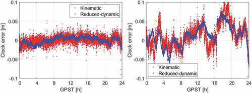
Figure 2 shows the clock estimates in the reduced-dynamic and kinematic modes based on the measurement geometry of GRACE FO-1 and the GPS satellites on 3 December 2019, expressed in meters. The CNES real-time products were used in the computed terms for both cases. To illustrate the influences of using real-time GNSS products, the left panel used the CNES real-time products in the simulated observations, i.e. not considering the term $\left|r_{L,JPL}-r_{FN}^s\right|-\left|r_{L,0}-r_{RT}^s\right|$ in Equations (11)(11) $\mathrm{\Delta }{\phi }_{IF,s}=\left|r_{L,JPL}-r_{FN}^s\right|-\left|r_{L,0}-r_{RT}^s\right|-c\times \left(\mathrm{\Delta }{\tilde{t}}_{FN}^s-\mathrm{\Delta }{\tilde{t}}_{RT}^s\right)+c\times \mathrm{\Delta }{\tilde{t}}_L+{\lambda }_{IF}\times {\tilde{N}}_{IF,s}+{\epsilon }_{\phi ,s}$(11) and (12(12) $\mathrm{\Delta }{p}_{IF,s}=\left|r_{L,JPL}-r_{FN}^s\right|-\left|r_{L,0}-r_{RT}^s\right|-c\times \left(\mathrm{\Delta }{\tilde{t}}_{FN}^s-\mathrm{\Delta }{\tilde{t}}_{RT}^s\right)+c\times \mathrm{\Delta }{\tilde{t}}_L+{\epsilon }_{p,s}$(12) ), while in the right panel the CODE final products were used to simulate LEO on-board observations as mentioned before. Error patterns of a few centimeters, up to about 1 dm, can be observed in the clock estimates in the right panel when the errors in the real-time products were considered. From Figure 2 it can also be observed that the clocks associated with the reduced-dynamic POD (blue dots) are smoother than those associated with the kinematic POD (red dots) due to the strong dynamic models applied. The root mean squares (RMS) of the clock errors amount to about 0.9 and 1.1 cm in the reduced-dynamic and the kinematic modes, respectively, when not considering the errors of the real-time GNSS products (left panel). They increased to about 2.9 and 3.3 cm when these errors were considered (right panel).

Figure 2. Clock errors caused by the GNSS estimation when (left) not considering and (right) considering the errors in the CNES real-time GPS products.

The stability of the clock errors caused by the GNSS processing was analyzed with the help of the modified Allan deviation (MDEV) (Riley 2008):

(13) $\mathrm{M}\mathrm{D}\mathrm{E}\mathrm{V}\left(\tau \right)=\sqrt{\frac{1}{2m^2{\tau }^2\left(N-3m+1\right)}\sum _{j=1}^{N-3m+1}{\left(\sum _{i=j}^{j+m-1}\left(x_{i+2m}-2x_{i+m}+x_i\right)\right)}^2}$(13)

where $x_i$ represents here the clock estimates at epoch $i$, and $N$ represents the number of the clock samples. The averaging time $\tau$ is calculated with the sampling interval ${\tau }_0$ and the averaging factor $m$:

(14) $\tau =m{\tau }_0$(14)

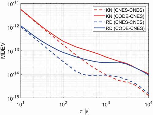
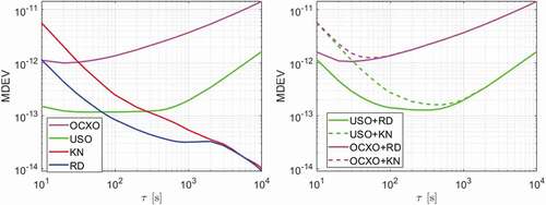
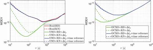
The MDEVs of the clock errors caused by the GNSS estimation are shown in Figure 3 when i) not considering (dashed lines) and ii) when considering (solid lines) the errors in the CNES real-time GPS products. The clock errors of two consecutive days of December 3 and 4, 2019 were used in the simulations. From Figure 3 it can be observed that the differences caused by the errors in the real-time products were mainly reflected in the degraded mid- and long-term clock stability (see the increase in the solid lines when $\tau$ is larger than 100 s). The clocks determined with the kinematic POD has worse short- and mid-term stabilities compared to those determined with the reduced-dynamic POD. In general, the MDEVs at the level of ${10}^{-12}$ with an averaging time of 10 s are worse than the short-term stability of the USOs at ${10}^{-13}$ (Dunn et al. 2003; Ko and Tapley 2010; Bertiger et al. 2003; Weinbach and Schön 2012). This suggests that in the short-term phase, the GNSS estimation errors play a more important role than the USO clock stability itself. This will be further discussed in the next sub-section.

Figure 3. MDEVs of the clock errors induced by the GNSS estimation. The CNES real-time GPS products were used in the estimation. The CODE final products (solid lines) and CNES real-time products (dashed lines) were used to simulate on-board LEO observations. Correspondingly, “CNES-CNES” means using the CNES real-time products in both the simulated and computed terms, while “CODE-CNES” means using the CODE final products in the simulated term, and the CNES real-time products in the computer term. KN and RD denote the kinematic and the reduced-dynamic modes, respectively.

3.2. Stability of the frequency oscillator

In this sub-section, the noise behaviors of the USO and OCXO are simulated with the help of the MDEVs. According to (Dunn et al. 2003; Ko and Tapley 2010; Bertiger et al. 2003; Weinbach and Schön 2012), the USOs on-board the GRACE satellites should generally have an Allan deviation of $1-3\times {10}^{-13}$ for an averaging time from 10 s to 1000 s. The frequency drift on-board the GRACE A and B satellites at 1000 days after launch amount to about $-2.8\times {10}^{-11}$/day and $-7.6\times {10}^{-12}$/day, respectively, and the USOs on-board the New Horizons (NH) spacecraft were also demonstrated to be around $\pm {10}^{-11}$/day at 700 days after launch (Weaver, Reinhart, and Wallis 2008). As such, to simulate the clock behaviors of a typical space-borne USO, flicker frequency modulation (FM) noise with an MDEV slope of zero at $1.5\times {10}^{-13}$ is overlapped with a frequency drift of ${10}^{-11}$/day, which has an MDEV slope of 1. The MDEV slopes of different noise types in a log-log plot are listed in Table 2 (Riley 2008). As shown in Figure 4, the simulated USO (blue line) is around $1-2\times {10}^{-13}$ between 10 s and 1000 s, and rises to higher values in the long-term with a slope of about 1 due to its frequency drift.

Figure 4. MDEVs of the simulated clock biases considering the stabilities of different frequency oscillators.

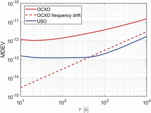
Table 2. MDEV slopes of different noise types in the log-log plot. PM and FM are short for phase modulation and frequency modulation, respectively

Noise type	Slope in MDEV
White PM noise	−1.5
Flicker PM noise	−1
White FM noise	−0.5
Flicker FM noise	0
Random-walk FM noise	0.5
Frequency drift	1

Compared to the USOs, the OCXOs generally have a worse stability in both the short- and long-term. The qualities of the OCXOs could vary according to their prices and manufacturers. In this study, we follow the performance of a space-system OCXO studied in (Hudson et al. 2019), with short-term stability of about ${10}^{-12}$ between 10 s and 100 s, and a random-walk FM noise with a slope of about 0.5 from 100 s to 10000 s (see the red solid line in Figure 4). The frequency drift of the tested space-system OCXO in (Hudson et al. 2019) has converged to about $-1.8\times {10}^{-11}$/day, which was also considered in the simulated OCXOs. This frequency drift, however, plays a less dominant role in the long-term than the random-walk FM noise (see the red dashed line in Figure 4).

Compared with the stability of the frequency oscillators, as shown in the left panel of Figure 5 (green and magenta lines), it is clear that the short-term clock stability is generally equally or more influenced by the GNSS estimation errors (red and blue lines). In contrast, the mid- to long-term stability is more influenced by the behaviors of the frequency oscillators themselves. The combined effects of both factors are illustrated in the right panel of Figure 5.

Figure 5. MDEVs of (left) the GNSS-induced errors and the biases of the frequency oscillators, and (right) the clock errors considering both factors.

3.3. Additional systematic effects

In addition to the GNSS estimation errors and the stability of the oscillators themselves, the clock behaviors can also be influenced by other factors, e.g. the measurement environment on-board the LEO satellite. In this section, two typical satellites GRACE FO-1 and SENTINEL-3B are used to show these additional systematic effects. The GRACE FO-1 has an orbital height of about 490 km, an eccentricity smaller than 0.0025 and an inclination of about 89${ }^{\circ }$ (GRACE-FO 2021). SENTINEL-3B has an orbital height of about 814.5 km, an eccentricity of about 0.0001 and an inclination of about 98.65${ }^{\circ }$ (Sentinel 2021). As an example, Figure 6 shows the large periodic behaviors of the satellite clock residuals on GRACE FO-1 on 3 December 2019, expressed in meters. The periods of the systematic effects in the left and right panels amount to about 12 h 22 min and 6 h 6 min, respectively. The period of the 12 h systematic effect, denoted as $T_{\alpha 1}$, was first estimated in the least-squares adjustment together with the polynomial coefficients $a_{j,\alpha 1}$ ($j$=0, 1, 2), amplitude (${\tilde{A}}_{\alpha 1}$) and phase (${\tilde{\phi }}_{\alpha 1}$):

(15) $\mathrm{E}\left(\mathrm{\Delta }\hat{t}\left(t_i\right)\right)=a_{0,\alpha 1}+a_{1,\alpha 1}\left(t_i-t_0\right)+a_{2,\alpha 1}{\left(t_i-t_0\right)}^2+{\tilde{A}}_{\alpha 1}\mathrm{s}\mathrm{i}\mathrm{n}\left(\frac{2\pi }{T_{\alpha 1}}\left(t_i-t_0\right)+{\tilde{\phi }}_{\alpha 1}\right)$(15)

where $\mathrm{\Delta }\hat{t}$ denotes the estimated receiver clock offset using raw observations of the satellite GRACE FO-1, i.e. the raw observations from the JPL at level L1A (Wen et al. 2019). A quadratic polynomial is used, as obvious frequency drifts exist in the USOs as discussed in Section 3.2. The CODE final products were used in a reduced-dynamic POD. $t_0$ and $t_i$ denote the start time of the processing and the time of the $i$-th epoch, respectively. The clock residuals of Equation (15)(15) $\mathrm{E}\left(\mathrm{\Delta }\hat{t}\left(t_i\right)\right)=a_{0,\alpha 1}+a_{1,\alpha 1}\left(t_i-t_0\right)+a_{2,\alpha 1}{\left(t_i-t_0\right)}^2+{\tilde{A}}_{\alpha 1}\mathrm{s}\mathrm{i}\mathrm{n}\left(\frac{2\pi }{T_{\alpha 1}}\left(t_i-t_0\right)+{\tilde{\phi }}_{\alpha 1}\right)$(15) , denoted as $\delta \hat{t}$, were used again to estimate the period of the 6 h systematic effect ($T_{\alpha 2}$) together with the coefficients $a_{j,\alpha 2}$ ($j$=0, 1, 2) of the remaining polynomial effects, the corresponding amplitude (${\tilde{A}}_{\alpha 2}$) and phase (${\tilde{\phi }}_{\alpha 2}$):

(16) $\mathrm{E}\left(\delta \hat{t}\left(t_i\right)\right)=a_{0,\alpha 2}+a_{1,\alpha 2}\left(t_i-t_0\right)+a_{2,\alpha 2}{\left(t_i-t_0\right)}^2+{\tilde{A}}_{\alpha 2}\mathrm{s}\mathrm{i}\mathrm{n}\left(\frac{2\pi }{T_{\alpha 2}}\left(t_i-t_0\right)+{\tilde{\phi }}_{\alpha 2}\right)$(16)

With the estimated $T_{\alpha 1}$ and $T_{\alpha 2}$, denoted as ${\hat{T}}_{\alpha 1}$ and ${\hat{T}}_{\alpha 2}$, introduced into the model, new polynomial coefficients ($a_{j,\alpha }$), amplitudes ($A_{\alpha 1},A_{\alpha 2}$) and clock phases (${\phi }_{\alpha 1}$, ${\phi }_{\alpha 2}$) were adjusted again with:

$\mathrm{E}\left(\mathrm{\Delta }\hat{t}\left(t_i\right)\right)=a_{0,\alpha }+a_{1,\alpha }\left(t_i-t_0\right)+a_{2,\alpha }{\left(t_i-t_0\right)}^2+A_{\alpha 1}\mathrm{s}\mathrm{i}\mathrm{n}\left(\frac{2\pi }{{\hat{T}}_{\alpha 1}}\left(t_i-t_0\right)+{\phi }_{\alpha 1}\right)$

(17) $+A_{\alpha 2}\mathrm{s}\mathrm{i}\mathrm{n}\left(\frac{2\pi }{{\hat{T}}_{\alpha 2}}\left(t_i-t_0\right)+{\phi }_{\alpha 2}\right)$(17)

Figure 6. Periodic behaviors of the GRACE FO-1 satellite clock residuals on 3 December 2019, with a period of about (left) 12 h and (right) 6 h. The blue lines shown in the left and right panels correspond to the clock residuals of $\mathrm{\Delta }\hat{t}$ (Equation 17(17) $+A_{\alpha 2}\mathrm{s}\mathrm{i}\mathrm{n}\left(\frac{2\pi }{{\hat{T}}_{\alpha 2}}\left(t_i-t_0\right)+{\phi }_{\alpha 2}\right)$(17) ) after detrending with the quadratic polynomial (with the coefficients $a_{j,\alpha }$) and after further detrending with the 12 h periodic term (with the coefficients $A_{\alpha 1}$, ${\phi }_{\alpha 1}$), respectively. The red lines correspond to the two periodic terms in Equation (17).

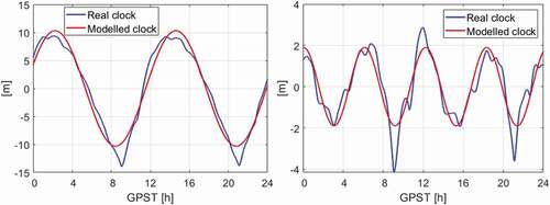
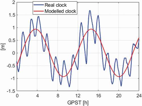
The amplitudes of the 12 h and 6 h systematic effects in Figure 6 amount to about 10.3 and 1.9 m, respectively. These large periodic residual behaviors were suspected to be linked to the temperature variations on the spacecraft (personal communication with the JPL). Similar long-term periodic effects can also be observed in the SENTINEL-3B clocks on 17 August 2018 (see Figure 7), however, with a much smaller amplitude of about 0.9 m and a shorter period of about 10 h 54 min. Independent assessments of the stability of the USO on-board Sentinel-3A & -3B has shown a correlation of its stability with the radiation, particularly over the so-called South Atlantic Anomaly (personal communication with the Copernicus POD Service)

Figure 7. Periodic behavior of the SENTINEL-3B satellite clock residuals on 14 August 2018, with a period of about 11 h.

Continuous daily processing from December 1 to 6, 2019 for GRACE FO-1 and from August 14 to 19, 2018 for SENTINEL-3B shows that the amplitudes and periods of the systematic effects also experience variations with time (see Table 3). Among them, large day-to-day period variation above 40 min was, e.g. observed in the systematic effects of SENTINEL-3B. These systematic effects do not really correspond to the GPS orbital period, and are likely to be satellite-specific. The physical reasons of the mid- and long-term effects expect further investigations in the future. In this study, they are assumed to be remained in the LEO satellite clocks and are considered in the clock prediction.

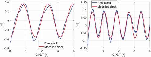
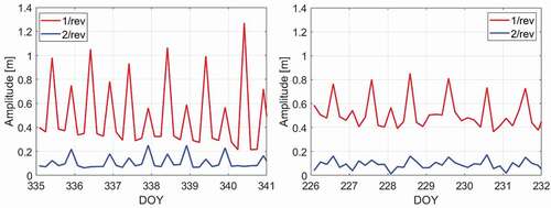
In addition to the mid- and long-term systematic effects as shown before, other short-term systematic effects also exist in the LEO satellite clocks. It is known that the clock mounted on-board a satellite has a frequency shift compared to the same clock on the ground, which is known as the relativistic effects. This would result in 1/rev and 2/rev periodic variations in the space-borne clocks. As observed in different LEO satellites, the amplitude of the 1/rev periodic effects typically amounts to a few nanoseconds (Bertiger et al. 2003; Larson et al. 2007). The 2/rev amplitudes are smaller and amount to, e.g. for the LEO satellites GRACE FO-1 and SENTINEL-3B, a few sub-nanoseconds. As an example, Figure 8 shows the 1/rev and 2/rev periodic effects in the GRACE FO-1 from 0:00 to 4:00 in GPST. To better retrieve the 1/rev and 2/rev effects, the amplitudes ($A_{\beta 1}$, $A_{\beta 2}$) and phases (${\phi }_{\beta 1}$, ${\phi }_{\beta 2}$) of the modeled clocks (red lines) were estimated with a fourth-order polynomial using 10 s clocks within 4 h:

$\mathrm{E}\left(\delta {\hat{t}}_2\left(t_i\right)\right)=a_{0,\beta }+a_{1,\beta }\left(t_i-t_0\right)+\cdots +a_{4,\beta }{\left(t_i-t_0\right)}^4+A_{\beta 1}\mathrm{s}\mathrm{i}\mathrm{n}\left(\frac{2\pi }{T_{\beta }}\left(t_i-t_0\right)+{\phi }_{\beta 1}\right)$

(18) $+A_{\beta 2}\mathrm{s}\mathrm{i}\mathrm{n}\left(\frac{4\pi }{T_{\beta }}\left(t_i-t_0\right)+{\phi }_{\beta 2}\right)$(18)

where $\delta {\hat{t}}_2$ denotes the clock residuals from Equation (17)(17) $+A_{\alpha 2}\mathrm{s}\mathrm{i}\mathrm{n}\left(\frac{2\pi }{{\hat{T}}_{\alpha 2}}\left(t_i-t_0\right)+{\phi }_{\alpha 2}\right)$(17) . The term $T_{\beta }$ denotes the LEO orbital period. The amplitudes of the 1/rev and 2/rev effects shown in Figure 8 reached about 0.36 m and 0.08 m, i.e. 1.2 ns and 0.3 ns, respectively. A shorter time interval and higher-older polynomials were used to extract the smaller 1/rev and 2/rev effects than those in the large systematic effects described before. This is caused by the disturbance of the Flicker FM noise, the other miss-modeled non-periodic effects, and the time-varying amplitudes of the 1/rev and 2/rev effects which will be discussed later in this section.

Figure 8. (Left) 1/rev and (right) 2/rev periodic effects in the GRACE FO-1 clocks on 3 December 2019 – note the difference in the y scale. The blue line in the left panel corresponds to $\delta {\hat{t}}_2$ (Equation 18(18) $+A_{\beta 2}\mathrm{s}\mathrm{i}\mathrm{n}\left(\frac{4\pi }{T_{\beta }}\left(t_i-t_0\right)+{\phi }_{\beta 2}\right)$(18) ) with the fourth-order polynomial removed, and the one in the right panel corresponds to the blue line in the left panel with the 1/rev term $A_{\beta 1}\mathrm{s}\mathrm{i}\mathrm{n}\left(\frac{2\pi }{T_{\beta }}\left(t_i-t_0\right)+{\phi }_{\beta 1}\right)$ (Equation 18(18) $+A_{\beta 2}\mathrm{s}\mathrm{i}\mathrm{n}\left(\frac{4\pi }{T_{\beta }}\left(t_i-t_0\right)+{\phi }_{\beta 2}\right)$(18) ) further removed. The red lines correspond to the two periodic terms in Equation (18).

Compared to the GNSS satellites, the LEO satellites are nearer to the Earth and are thus more influenced by the Earth’s gravitational potential. Instead of using the general form ($-2\frac{rv}{c^2})$ with $r$ and $v$ denoting the satellite position and velocity vectors, a more exact expression was developed in (Larson et al. 2007), considering also the $J_2$ effects caused by the Earth’s oblateness. The correction has shown to be able to reduce the 2/rev terms, but could enlarge the 1/rev power. The 1/rev effects of, e.g. GRACE A and B, were suspected to be related to the voltage variations on the spacecraft. Having a look at the amplitudes of the 1/rev and 2/rev effects of GRACE FO-1 from December 1 to 6, 2019 (see the left panel of Figure 9), half-daily pulses can be observed. For SENTINEL-3B as shown in the right panel of Figure 9, daily pulses are also observable. This suggests again that the 1/rev and/or 2/rev behaviors in the LEO clocks could be linked to other effects in the local measurement environment of the spacecraft, and might not be able to be perfectly cleaned by the MPC and then re-corrected by the ground-users. Considering the 1/rev periodic effects that could be possibly related to the high correlation between the radial orbits and the satellite clocks, we note that the radial orbital errors processed for, e.g. the GRACE FO-1 on 3 December 2019, have an RMS of about 1.2 cm with respect to the reference orbits provided by the JPL. The corresponding effects on clocks caused by the correlation cannot thus reach an amplitude of a few decimeters.

Figure 9. Amplitudes of the 1/rev and 2/rev periodic effects on the LEO satellites (left) GRACE FO-1 and (right) SENTINEL-3B.

The satellite-specific periodic effects mentioned above remain in the clock estimates. Before the physical reasons of these effects are clearly understood and the corresponding parameters, e.g. the temperature or voltage parameters can be broadcast to users, one cannot perfectly correct them on the ground, and thus needs to be considered in the clock prediction. For this purpose, in this study, several periodic effects are overlapped in the simulations. The simulated periodic clock effect $\mathrm{\Delta }{t}_p$ is expressed as follows:

(19) $\mathrm{\Delta }{t}_p\left(t_i\right)=\underset{\mathrm{\Delta }{t}_{p,\alpha }}{\underbrace{\sum _{j=1}^k\left(A_{\alpha j}\mathrm{s}\mathrm{i}\mathrm{n}\left(\frac{2\pi }{T_{\alpha j}}\left(t_i-t_0\right)\right)\right)}}+\underset{\mathrm{\Delta }{t}_{p,\beta }}{\underbrace{A_{\beta 1}\mathrm{s}\mathrm{i}\mathrm{n}\left(\frac{2\pi }{T_{\beta }}\left(t_i-t_0\right)\right)+A_{\beta 2}\mathrm{s}\mathrm{i}\mathrm{n}\left(\frac{4\pi }{T_{\beta }}\left(t_i-t_0\right)\right)}}$(19)

where $k$ denotes the number of the simulated mid- and long-term effects, which will be explained in Section 4. In the simulations, the amplitude and period of each periodic effect were set to be constant, as its variation could differ for different satellites and the reason is not yet clear. Note that it is possible to use methods such as FFT to infer the number of periodic effects to be considered in $\mathrm{\Delta }{t}_{p,\alpha }$ for the investigated satellite clocks. The effect of modeling non-pronounced effects, such as systematic effects of other periods, is however yet to be examined in presence of the Flicker FM noise of the USOs and the other non-periodic effects.

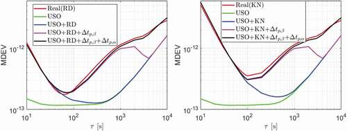
Figure 10 shows the MDEVs of the real clocks of GRACE FO-1 on December 3–4, 2019 and the simulated clocks adding different effects, considered in the steps of computations. The real clocks were estimated using the CNES real-time GPS products, with the clocks re-aligned to the reference clock of the CODE final products on 3 December 2019. The boundary effects between consecutive days in the clock estimates were merged. From Figure 10, it can be observed that the short-term noise of the USO approaches the real clocks by adding the GNSS estimation errors (see the green and blue lines). To better understand the differences between the real and the simulated clocks, the periods and amplitudes of the systematic effects derived from the real data of GRACE FO-1 over the two test days were applied in the simulations. Above the blue line, adding the 1/rev and 2/rev periodic effects $\mathrm{\Delta }{t}_{p,\beta }$ (Equation 19(19) $\mathrm{\Delta }{t}_p\left(t_i\right)=\underset{\mathrm{\Delta }{t}_{p,\alpha }}{\underbrace{\sum _{j=1}^k\left(A_{\alpha j}\mathrm{s}\mathrm{i}\mathrm{n}\left(\frac{2\pi }{T_{\alpha j}}\left(t_i-t_0\right)\right)\right)}}+\underset{\mathrm{\Delta }{t}_{p,\beta }}{\underbrace{A_{\beta 1}\mathrm{s}\mathrm{i}\mathrm{n}\left(\frac{2\pi }{T_{\beta }}\left(t_i-t_0\right)\right)+A_{\beta 2}\mathrm{s}\mathrm{i}\mathrm{n}\left(\frac{4\pi }{T_{\beta }}\left(t_i-t_0\right)\right)}}$(19) ) effectively shortened the distance between the MDEVs of the simulated and real clocks between about 100 s and 4000 s (see the magenta lines). The mid- and long-term period effects $\mathrm{\Delta }{t}_{p,\alpha }$ (Equation 19(19) $\mathrm{\Delta }{t}_p\left(t_i\right)=\underset{\mathrm{\Delta }{t}_{p,\alpha }}{\underbrace{\sum _{j=1}^k\left(A_{\alpha j}\mathrm{s}\mathrm{i}\mathrm{n}\left(\frac{2\pi }{T_{\alpha j}}\left(t_i-t_0\right)\right)\right)}}+\underset{\mathrm{\Delta }{t}_{p,\beta }}{\underbrace{A_{\beta 1}\mathrm{s}\mathrm{i}\mathrm{n}\left(\frac{2\pi }{T_{\beta }}\left(t_i-t_0\right)\right)+A_{\beta 2}\mathrm{s}\mathrm{i}\mathrm{n}\left(\frac{4\pi }{T_{\beta }}\left(t_i-t_0\right)\right)}}$(19) ) were further added to the simulated clocks to reduce its difference from the real clocks after 1000 s (see the black lines).

Figure 10. MDEVs of the real and simulated clocks for GRACE FO-1 on December 3–4, 2019 in (left) the reduced-dynamic mode and (right) the kinematic mode.

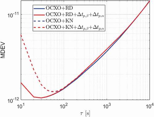
The periodic effects with the same amplitudes as used in Figure 10, however, do not significantly influence the simulated OCXO due to its worse mid- and long-term stabilities. As shown in Figure 11, the simulated OCXO considering the periodic effects (red lines) are almost the same as those not considering these effects (blue lines).

Figure 11. MDEVs of the simulated OCXOs with and without considering the periodic effects.

In addition to the periodic effects modeled in this sub-section, other miss-modeled effects, e.g. the high-order polynomials removed before assessing the 1/rev and the 2/rev effects (Equation 18(18) $+A_{\beta 2}\mathrm{s}\mathrm{i}\mathrm{n}\left(\frac{4\pi }{T_{\beta }}\left(t_i-t_0\right)+{\phi }_{\beta 2}\right)$(18) ), could also influence the prediction. This will be discussed in Section 4.2.

3.4. Stability of the time reference

In the clock prediction, it is always good to use a time reference that is significantly more stable than the clock itself. Different from the very stable time reference in the final clock products of, e.g. CODE and IGS, the time reference of the real-time GNSS products, however, does not always meet this requirement. Figure 12 shows the stabilities of the time references in different real-time clock products based on the corresponding daily clock files from December 1 to 7, 2019. The MDEVs were computed using the epoch-mean clock differences between the real-time and the CODE final clocks. Note that the CODE final clocks were referred to selected Hydrogen-Masers (Bock et al. 2009), which exhibit very good stabilities. As a comparison, the MDEVs of the epoch-mean clock differences were also shown for the IGS and the CODE final clocks (yellow line). As the tested real-time GPS clock products all have good precision of a few centimeters (Zhang et al. 2019; Kazmierski, Sonica, and Hadas 2018; IGS 2020), the relatively high MDEVs of the epoch-mean clock differences are mainly caused by the stabilities of the time references themselves. To clarify this, the MDEVs of the simulated white PM noise with a formal standard deviation of the mean clock difference (${\sigma }_D$) were also illustrated with the magenta line, having the precision of the real-time clocks (${\sigma }_{RT}$) set to 5 cm as an example:

(20) ${\sigma }_D=\sqrt{\frac{{\sigma }_{RT}^2+{\sigma }_{CODE}^2}{n}}\approx \frac{{\sigma }_{RT}}{\sqrt{n}}$(20)

where the formal standard deviation of the CODE final products ${\sigma }_{CODE}$ is much smaller than that of the real-time products, and thus is ignored. The term $n$ represents the number of the GPS satellites used for the differencing at the corresponding epoch. It was approximated to 30 here based on the epoch-mean satellite numbers having valid real-time clocks and CODE final clocks over the test period for different products.

Figure 12. MDEVs of the epoch-mean clock differences between different real-time clock products and the CODE final clocks. The dashed line refers to the MDEVs of the white PM noise with a standard deviation of ${\sigma }_D$ (Equation 20).

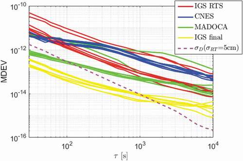
From Figure 12, it can be observed that the short-term stabilities of some of the real-time time references are worse than those shown in Figure 10. Note that the shortest averaging time in Figure 12 is 30 s. Applying the GPS clocks of these real-time products would implicitly include these instabilities in the estimated LEO satellite clocks, as the GPS satellite clocks in these products form the time reference of the LEO clock estimates. To illustrate the influences of the time reference, the epoch-mean clock differences between the CNES real-time clocks and the CODE final clocks on December 3–4, 2019, were introduced into the simulated clocks. Note that the CODE final clocks on 4 December 2019, were re-aligned to its reference clock on 3 December 2019. For the MDEVs of the real clock estimates (see the red lines in the left panel of Figure 13), the original time reference in the real-time CNES products was used. As shown in Figure 13, the influence of an unstable time reference is visible for both the simulated USO and OCXO. By adding the shift of the time reference into the simulated USO (see the blue lines in the left panel), the corresponding MDEVs approach those of the real clock estimates based on the CNES real-time products (see the red lines almost overwritten by the blue lines in the left panel). For both the kinematic and the reduced-dynamic modes, the short-term stability of the time reference plays a dominant role compared to other effects. To ease the clock prediction, it is thus suggested to use the real-time GNSS products with a stable time reference. In this study, the influences of an actual time reference, i.e. that of the CNES real-time products over December 3–4, 2019, are discussed in Section 4 as a representative example.

Figure 13. MDEVs of the simulated clocks for (left) USO and (right) OCXO with and without adding the errors of the time reference of the real-time CNES clocks on December 3–4, 2019.

As a summary, the simulated clock $\mathrm{\Delta }{t}_{all}$ can be expressed as:

(21) $\mathrm{\Delta }{t}_{all}=\mathrm{\Delta }\hat{t}+\mathrm{\Delta }{t}_o+\mathrm{\Delta }{t}_p+\mathrm{\Delta }{t}_r$(21)

where $\mathrm{\Delta }\hat{t}$ refers to the clock errors caused by the GNSS estimation, $\mathrm{\Delta }{t}_o$ denotes the noise of the frequency oscillator itself, $\mathrm{\Delta }{t}_p$ represents the simulated periodic effects (Equation 19(19) $\mathrm{\Delta }{t}_p\left(t_i\right)=\underset{\mathrm{\Delta }{t}_{p,\alpha }}{\underbrace{\sum _{j=1}^k\left(A_{\alpha j}\mathrm{s}\mathrm{i}\mathrm{n}\left(\frac{2\pi }{T_{\alpha j}}\left(t_i-t_0\right)\right)\right)}}+\underset{\mathrm{\Delta }{t}_{p,\beta }}{\underbrace{A_{\beta 1}\mathrm{s}\mathrm{i}\mathrm{n}\left(\frac{2\pi }{T_{\beta }}\left(t_i-t_0\right)\right)+A_{\beta 2}\mathrm{s}\mathrm{i}\mathrm{n}\left(\frac{4\pi }{T_{\beta }}\left(t_i-t_0\right)\right)}}$(19) ), and $\mathrm{\Delta }{t}_r$ refers to the errors caused by the time reference. In Section 4.2, the clock prediction using an actual real-time time reference (as selected in Figure 13) is compared with the case without considering the influences of the time reference, which could happen when the time reference is much more stable than the tested clock.

4. Clock prediction

Based on the systematic effects in LEO satellite clocks described in Section 3.3, the USOs are predicted following the model expressed as:

$\mathrm{\Delta }\check{t}\left(t_i-t_0\right)={\hat{a}}_0+{\hat{a}}_1\left(t_i-t_0\right)+\cdots +{\hat{a}}_m{\left(t_i-t_0\right)}^m+\sum _{j=1}^k{\hat{A}}_{\alpha j}\mathrm{s}\mathrm{i}\mathrm{n}\left(\frac{2\pi }{{\hat{T}}_{\alpha j}}\left(t_i-t_0\right)+{\hat{\phi }}_{\alpha j}\right)$

(22) $+\sum _{j=1}^2{\hat{A}}_{\beta j}\mathrm{s}\mathrm{i}\mathrm{n}\left(\frac{2j\pi }{T_{\beta }}\left(t_i-t_0\right)+{\hat{\phi }}_{\beta j}\right)$(22)

where $k$ denotes the number of the mid- and/or long-term periodic effects, which could be satellite specific. The value of $k$ can, e.g. be obtained based on suggestions of the institution monitoring the satellite or analysis of previous clock data of the corresponding satellite. The parameters of the periodic effects and the polynomial coefficients are estimated in the following procedure, applied in consecutive steps:

• Step 1 (Equations 15(15) $\mathrm{E}\left(\mathrm{\Delta }\hat{t}\left(t_i\right)\right)=a_{0,\alpha 1}+a_{1,\alpha 1}\left(t_i-t_0\right)+a_{2,\alpha 1}{\left(t_i-t_0\right)}^2+{\tilde{A}}_{\alpha 1}\mathrm{s}\mathrm{i}\mathrm{n}\left(\frac{2\pi }{T_{\alpha 1}}\left(t_i-t_0\right)+{\tilde{\phi }}_{\alpha 1}\right)$(15) and 16(16) $\mathrm{E}\left(\delta \hat{t}\left(t_i\right)\right)=a_{0,\alpha 2}+a_{1,\alpha 2}\left(t_i-t_0\right)+a_{2,\alpha 2}{\left(t_i-t_0\right)}^2+{\tilde{A}}_{\alpha 2}\mathrm{s}\mathrm{i}\mathrm{n}\left(\frac{2\pi }{T_{\alpha 2}}\left(t_i-t_0\right)+{\tilde{\phi }}_{\alpha 2}\right)$(16) ): Estimate the periods of the mid- and long-term effects ${\hat{T}}_{\alpha j}$ with a quadratic polynomial using a long fitting interval of 24 h;

• Step 2 (Equation 17(17) $+A_{\alpha 2}\mathrm{s}\mathrm{i}\mathrm{n}\left(\frac{2\pi }{{\hat{T}}_{\alpha 2}}\left(t_i-t_0\right)+{\phi }_{\alpha 2}\right)$(17) ): Introduce ${\hat{T}}_{\alpha j}$, and estimate the parameters of the mid- and long-term periodic effects ${\hat{A}}_{\alpha j}$ and ${\hat{\phi }}_{\alpha j}$ with a quadratic polynomial using the same fitting interval as in Step 1;

• Step 3 (Equation 18(18) $+A_{\beta 2}\mathrm{s}\mathrm{i}\mathrm{n}\left(\frac{4\pi }{T_{\beta }}\left(t_i-t_0\right)+{\phi }_{\beta 2}\right)$(18) ): Introduce ${\hat{T}}_{\alpha j}$, ${\hat{A}}_{\alpha j}$ and ${\hat{\phi }}_{\alpha j}$, and estimate the parameters of the 1/rev and 2/rev effects (${\hat{A}}_{\beta j}$ and ${\hat{\phi }}_{\beta j}$) with a fourth-order polynomial using a fitting interval of 4 h;

• Step 4: Introduce ${\hat{T}}_{\alpha j}$, ${\hat{A}}_{\alpha j}$, ${\hat{\phi }}_{\alpha j}$, ${\hat{A}}_{\beta j}$ and ${\hat{\phi }}_{\beta j}$ at their corresponding fitting intervals, and estimate the polynomial coefficients ${\hat{a}}_j$ ($j=0,\cdots ,m$). The polynomial coefficient $m$ is tested from 1 to 3, and the polynomial fitting interval is tested for different lengths from $10\left(m+2\right)$ s to 24 h;

• Step 5: For each tested prediction interval and polynomial degree, the polynomial fitting interval that delivers the smallest RMS of the prediction errors is considered as the most suitable one. The polynomial fitting in Step 4 is then repeated using this fixed polynomial fitting interval for the corresponding prediction interval and polynomial degree;

• Step 6 (Equation 22(22) $+\sum _{j=1}^2{\hat{A}}_{\beta j}\mathrm{s}\mathrm{i}\mathrm{n}\left(\frac{2j\pi }{T_{\beta }}\left(t_i-t_0\right)+{\hat{\phi }}_{\beta j}\right)$(22) ): Perform the prediction based on all the estimated coefficients mentioned above. Note that ${\hat{A}}_{\beta j}$ and ${\hat{\phi }}_{\beta j}$ at the latest fitting interval are used in the prediction.

For the OCXOs, as shown in Figure 11, the systematic effects with the amplitudes studied in this contribution do not significantly influence their mid- and long-term stabilities. As such, their prediction is performed only based on the polynomial fitting from the steps 4 to 6. In the next two sub-sections, the prediction errors are discussed based on the simulated and real clocks.

4.1. Prediction errors using simulated clocks

Based on the simulated clocks generated in Section 3 and the model mentioned before, the prediction errors were assessed for a prediction interval varying from 10 s to 1 h. The simulated clocks covered 48 h with a sampling interval of 10 s. The beginning of the fitting interval of 24 h was shifted by 1 min for each set of the predictions, such that 1380 samples were used in total. The periods of the long-term ($T_{\alpha 1}$) and mid-term ($T_{\alpha 2}$) effects (Equation 19(19) $\mathrm{\Delta }{t}_p\left(t_i\right)=\underset{\mathrm{\Delta }{t}_{p,\alpha }}{\underbrace{\sum _{j=1}^k\left(A_{\alpha j}\mathrm{s}\mathrm{i}\mathrm{n}\left(\frac{2\pi }{T_{\alpha j}}\left(t_i-t_0\right)\right)\right)}}+\underset{\mathrm{\Delta }{t}_{p,\beta }}{\underbrace{A_{\beta 1}\mathrm{s}\mathrm{i}\mathrm{n}\left(\frac{2\pi }{T_{\beta }}\left(t_i-t_0\right)\right)+A_{\beta 2}\mathrm{s}\mathrm{i}\mathrm{n}\left(\frac{4\pi }{T_{\beta }}\left(t_i-t_0\right)\right)}}$(19) ) were set to 12 h and 6 h, respectively, in the simulations following the given example of GRACE FO-1. Their corresponding amplitudes ($A_{\alpha 1}$, $A_{\alpha 2}$) were tested for 0 and 10 m for the 12 h effect, and 0 and 2 m for the 6 h effect, allowing these effects also to be absent and the corresponding Steps 1 and 2 mentioned above to be disabled. The amplitudes of the 1/rev ($A_{\beta 1}$) and 2/rev ($A_{\beta 2}$) effects were set to 0.5 and 0.1 m, respectively. The LEO orbital period $(T_{\beta }$) was set to that of the GRACE FO-1 on 3 December 2019, which amounts to about 1.6 h. Note that by evaluating the prediction errors, the GNSS estimation errors were not contained in the “true” clocks.

As shown in Table 4, the analysis started from a simple scenario (Scenario A) for the reduced-dynamic mode with $A_{\alpha 1}$ and $A_{\alpha 2}$ set to 0 m, and with the influences of the time reference not considered. The other effects were then added step-by-step to the simulated clocks. Figure 14 shows an example for the simulated USO under different scenarios. A linear polynomial was fitted in the steps 4–6. The most significant increase in the RMSE of the predicted clocks appears when considering the influences of the time reference, i.e. the CNES real-time clock reference on December 3–4, 2019 here. In the right panel of Figure 14, the RMSE of the predicted clocks is shown when only a linear polynomial was used for the modeling. A dramatic increase of meters can be observed, especially when the large mid- and long-term periodic effects are present (Scenarios B-E). The differences between the left and the right panels of Figure 14 indicate that modeling the periodic effects is helpful to reduce the mid- and long-term prediction errors for USOs having such systematic effects.

Figure 14. RMSE of the predicted USOs under different scenarios when applying (left) the proposed model with a linear polynomial in the steps 4–6 and (right) when only applying a linear polynomial.

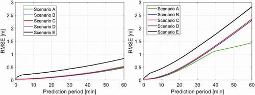
Table 3. Characteristics of the mid- and long-term systematic effects in the clocks of GRACE FO-1 from December 1 to 6, 2019 and in the clocks of SENTINEL-3B from August 14 to 19, 2018

Satellite	Parameter	Mean value	Min. day-to-day variation	Max. day-to-day variation
GRACE FO-1	Period (12 h)	12 h 11 min	<1 min	24 min
	Amplitude (12 h)	10.22 m	0.07 m	0.47 m
	Period (6 h)	6 h 5 min	<1 min	9 min
	Amplitude (6 h)	2.12 m	0.04 m	0.39 m
SENTINEL-3B	Period (11 h)	10 h 50 min	<1 min	42 min
	Amplitude (11 h)	1.29 m	0.24 m	0.46 m

Table 4. Scenarios for clock prediction based on the simulated LEO clocks

Scenario ID	Estimation mode	Amplitudes of periodic effects		Time reference	Prediction Steps
		1/rev and 2/rev	Long- and mid-term
A	Reduced-dynamic	0.5 m, 0.1 m	–	–	3–6, 4–6
B	Reduced-dynamic	0.5 m, 0.1 m	10 m, 2 m	–	1–6, 4–6
C	Kinematic	0.5 m, 0.1 m	10 m, 2 m	–	1–6, 4–6
D	Reduced-dynamic	0.5 m, 0.1 m	10 m, 2 m	CNES real-time	1–6, 4–6
E	Kinematic	0.5 m, 0.1 m	10 m, 2 m	CNES real-time	1–6, 4–6

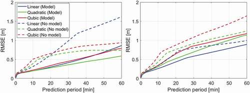
Based on Scenario D, the differences when applying polynomials of different degrees are shown in the left panel of Figure 15. Compared to the cases when only using the polynomial fitting model (dashed lines), the benefits of applying the proposed model (solid lines) are shown to be significant for all the three tested polynomial degrees, especially in the long-term. The quadratic and cubic polynomials appear to be the better options for prediction period over 15 min. From the right panel of Figure 15, it can be concluded that a longer prediction interval and a higher polynomial degree tends to require a longer polynomial fitting interval.

Figure 15. (Left) RMSE of the predicted USOs under scenario D and (right) the best suitable polynomial fitting time. The solid and dashed lines represent the cases when the proposed model was used and when only the polynomial fitting was applied, respectively.

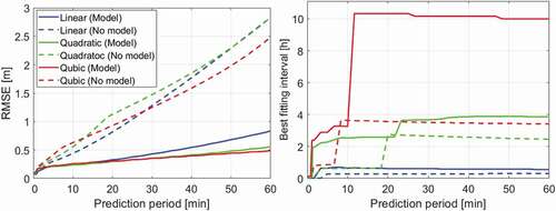
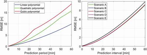
For the OCXO, as mentioned before, only the polynomial fitting was attempted due to its bad mid- and long-term stabilities. The left panel of Figure 16 shows the RMSE of the predicted OCXO under Scenario D using polynomials with a degree from one to three. The linear polynomial becomes the best option for OCXOs with higher random-walk FM noise than the frequency drift (Figure 4). Compared to the USO under the same scenario, the mid- and long-term prediction errors are much larger for the OCXO due to the worse stability of the oscillator. Adding different effects from Scenarios A to E, as shown in the right panel of Figure 16, the largest increase again comes from the influences of the time reference.

Figure 16. RMSE of the predicted OCXOs (left) under Scenario D applying polynomials of different degrees and (right) under different scenarios applying a linear polynomial. Note the different RMSE scales for the two plots.

The error budget of the LEO clock prediction errors is summarized in Table 5 from Scenarios B to E, i.e. assuming a very stable time reference can be used in the Scenarios B and C, and for Scenarios D and E considering the influences of the time reference of a typical real-time clock product, here the CNES product, on December 3–4, 2019. For the purpose of consistency between the two clock types, and also between the simulated and real clocks that will be discussed in the next sub-section, a linear polynomial was used for both clock types applying, and not applying the proposed model. The benefit of applying the proposed model compared to the case when only applying the polynomial fitting is calculated as:

(23) $B=\frac{{\sigma }_p-{\sigma }_m}{{\sigma }_p}$(23)

Table 5. RMSE of the predicted clocks, the best suitable polynomial fitting time and the benefit of applying the proposed model (Equation 23(23) $B=\frac{{\sigma }_p-{\sigma }_m}{{\sigma }_p}$(23) ). The results for the reduced-dynamic (Scenarios B and D) and the kinematic modes (Scenarios C and E) are separated by a slash “/”, respectively

		Scenarios B and C			Scenarios D and E
Clock type	Prediction period	RMSE [m]	Fitting time [s]	Benefit [%]	RMSE [m]	Fitting time [s]	Benefit [%]
USO	30 s	0.03/0.04	1000/300	1.1/0.6	0.07/0.07	50/40	0.0/0.0
	1 min	0.03/0.04	900/400	1.1/1.8	0.11/0.11	50/50	0.0/-0.0
	10 min	0.05/0.06	400/600	60.2/59.6	0.25/0.25	2300/2200	44.3/43.9
	30 min	0.17/0.19	300/600	79.9/78.5	0.43/0.43	2200/2200	66.4/66.0
	1 h	0.48/0.51	300/400	79.3/78.4	0.83/0.83	2000/2000	70.5/70.5
OCXO	30 s	0.04/0.04	30/60	–	0.08/0.08	50/40	–
	1 min	0.05/0.06	30/60	–	0.11/0.11	50/50	–
	10 min	0.67/0.68	40/80	–	0.94/0.95	50/300	–
	30 min	3.29/3.33	40/80	–	3.75/3.75	300/300	–
	1 h	9.25/9.29	40/80	–	9.92/9.92	300/300	–

where ${\sigma }_m$ and ${\sigma }_p$ denote the RMSE of the predicted clocks applying the proposed model and applying only the polynomial fitting model, respectively.

Based on Table 5, the RMSE of the predicted USOs under Scenarios D/E amount to about 0.1 m and 0.8 m for prediction periods of 1 min and 1 h, respectively. Without considering the influences of the time reference (Scenarios B and C), the RMS of the short-term prediction errors at 1 min is at a few centimeters for both clock types. The benefits of applying the proposed model are significant for the mid- and long-term predictions, i.e. ranging from about 40% to 70% for Scenarios D and E. For the simulated OCXOs, the RMSE of the short-term prediction is at a similar level but reached about 10 m at a prediction interval of 1 h. The differences between the reduced-dynamic and the kinematic modes are generally not significant.

4.2. Miss-modeled effects in real clocks

In the simulations, the good prediction results were achieved based on the assumption that the systematic effects in the simulated clocks perfectly follow the described model in Equation (22)(22) $+\sum _{j=1}^2{\hat{A}}_{\beta j}\mathrm{s}\mathrm{i}\mathrm{n}\left(\frac{2j\pi }{T_{\beta }}\left(t_i-t_0\right)+{\hat{\phi }}_{\beta j}\right)$(22) . This, however, does not totally match the real situation. In addition to the varying amplitudes and periods of the periodic effects as discussed in Section 3.3, other systematic effects or high-order polynomials, e.g. those removed before assessing the 1/rev and 2/rev effects, could exist in the clock estimates. These satellite-specific miss-modeled effects could degrade the mid- and long-term prediction results.

To assess the resulted differences in the clock prediction, the proposed model was used for prediction of the real clock estimates of SENTINEL-3B on August 14–15, 2018 and GRACE FO-1 on December 3–4, 2019. The processing was performed in the reduced-dynamic processing mode (as the more accurate approach than the kinematic mode) based on the CNES real-time GPS products. Accordingly, the clock estimates of a USO was simulated based on Scenario D (Table 4). 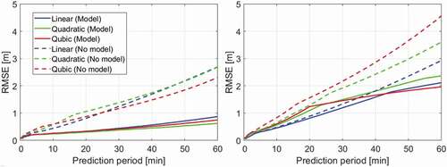The number of the mid- and long-term periodic effects $k$ (see Equation 22)(22) $+\sum _{j=1}^2{\hat{A}}_{\beta j}\mathrm{s}\mathrm{i}\mathrm{n}\left(\frac{2j\pi }{T_{\beta }}\left(t_i-t_0\right)+{\hat{\phi }}_{\beta j}\right)$(22) was set to two and one for GRACE FO-1 and SENTINEL-3B, respectively. The periodic effects of the USOs were simulated based on the mean amplitudes and periods of the corresponding satellite on the test days. Figure 17 shows the RMSE of the predicted clocks for SENTINEL-3B based on the simulated (left) and real clock estimates (right). The solid lines represent the cases when the proposed prediction model was used, and the dashed lines represent the cases using only the polynomial fitting. First, it is observable that the proposed model has largely reduced the prediction errors for both the simulated and real clocks, i.e. mostly by a few decimeters for mid- and long-term prediction. The miss-modeled effects remaining in the real clocks have generally led to degradations in the real clock prediction. Still, using the real clocks, the RMSE applying the proposed model with a linear polynomial (the blue solid line in the right panel) is generally at sub-dm to meter-level for a prediction interval of 1 h.

Figure 17. RMSE of the predicted clocks for SENTINEL-3B on August 14–15, 2018 using (left) the simulated clocks and (right) the real clock estimates. The solid and dashed lines represent the cases when the proposed model was used and when only the polynomial fitting was applied, respectively.

The miss-modeled effects are satellite-specific and could be larger than those in SENTINEL-3B. This can, e.g. clearly be observed when comparing the right panel of Figure 6 for GRACE FO-1 and Figure 7 for SENTINEL-3B. Figure 18 shows the RMSE of the predicted clocks for GRACE FO-1 on December 3–4, 2019 when using the simulated and real clocks. The increase in RMSE can be observed in both the solid and dashed lines when real data was used. Nevertheless, as shown in the right panel of Figure 18, the benefits when applying the proposed model are significant for the real clock prediction.

Figure 18. RMSE of the predicted clocks for GRACE FO-1 on December 3–4, 2019 using (left) the simulated clocks and (right) the real clock estimates. The solid and dashed lines represent the cases when the proposed model was used and when only the polynomial fitting was applied, respectively.

The error budget of the real clock prediction is summarized in Table 6. A linear polynomial was used for both satellites applying or not applying the proposed model. For Scenarios B and C, the CNES real-time clocks were re-referenced to the very stable CODE reference clocks on one of the two test days, so that the influences of the time reference can be considered as removed. Note that the “true” clocks at the prediction time were taken as the GNSS-based clock estimates, which contain the GNSS estimation errors having also the systematic effects shown in the right panel of Figure 2. This explains the optimistic short-term prediction results in the Scenarios B and C compared to those in the simulations. For Scenarios D and E considering the influences of the time reference, the short-term real clock prediction of 1 min has an RMSE of about 0.1 m, which is similar to those shown in the simulations. Depending on the complexity of the miss-modeled effects, the long-term prediction of 1 h could range from about 1 m to 2 m in the tested cases. The benefits of applying the proposed model are less than those in the simulations. Still, they reached about 5%-30% in Scenarios D/E for mid- and long-term prediction.

Table 6. RMSE of the predicted clocks, the best suitable polynomial fitting time and the benefit of applying the proposed model (Equation 23(23) $B=\frac{{\sigma }_p-{\sigma }_m}{{\sigma }_p}$(23) ) based on the real LEO clock estimates. The results for the reduced-dynamic and the kinematic modes are separated by “/”, respectively

		Scenarios B and C			Scenarios D and E
Satellite	Prediction period	RMSE [m]	Fitting time [s]	Benefit [%]	RMSE [m]	Fitting time [s]	Benefit [%]
SENTINEL-3B	30 s	0.01/0.01	50/60	0.3/0.2	0.03/0.03	60/60	−0.1/-0.1
	1 min	0.01/0.02	60/100	0.7/0.6	0.09/0.09	70/70	0.0/0.0
	10 min	0.13/0.15	200/300	17.2/17.3	0.26/0.26	1100/1100	23.0/23.0
	30 min	0.46/0.47	400/600	37.9/36.4	0.58/0.58	5600/5600	27.1/27.3
	1 h	0.80/0.79	5700/5700	14.2/14.9	0.89/0.89	5900/5900	10.1/10.7
GRACE FO-1	30 s	0.004/0.01	70/100	0.5/0.2	0.07/0.07	50/50	0.1/0.1
	1 min	0.01/0.02	70/200	1.5/1.0	0.10/0.10	50/50	0.0/0.0
	10 min	0.14/0.17	60/100	7.1/5.3	0.46/0.46	1000/1000	4.8/5.1
	30 min	0.78/0.83	60/100	12.7/12.1	1.20/1.20	1000/1100	10.4/10.5
	1 h	1.94/1.94	5700/5700	18.4/20.3	2.11/2.10	5800/5800	27.8/28.3

5. Conclusions

The ongoing development of thousands of LEO satellites forming mega-constellations motivates the investigations in their augmentation of the current GNSS for positioning. They can enable positioning in challenging environments such as urban canyons, and help in reducing the convergence time for PPP. To realize the benefits brought by the LEO mega-constellations for, e.g. PPP, the orbit and the clock products are essential. This contribution studied the GNSS clock estimates of typical LEO satellites. To facilitate this investigation, two types of LEO satellite clocks, i.e. the USO and the OCXO, were simulated. A model was proposed to describe the possible systematic effects remaining in the LEO clocks. Prediction errors of up to 1 h were compared when applying the proposed model versus using the simple polynomial fitting model under different conditions.

The LEO clock prediction was performed based on the high-accuracy LEO clock estimates in the reduced-dynamic or the kinematic POD. The stability of the estimated LEO clocks was found to be related to four different factors, i.e. the GNSS estimation errors, the stability of the frequency oscillator itself, the systematic effects caused by relativistic effects or other factors, and stability of the real-time time reference. Among the four sources, the GNSS estimation errors and the stability of the real-time time reference were found to be the key factors for the short-term stability. For the mid- and long-term stabilities, the behavior of the oscillator itself and the systematic effects play a more important role.

The prediction errors of the two clock types were investigated for prediction period of up to 1 h for possible low-sampled broadcast messages. For the simulated USOs without considering any miss-modeled effects, using the proposed model (with a linear polynomial), the RMSE of the predicted clocks amount to about 0.1 m and 0.8 m for prediction periods of 1 min and 1 h, respectively. Note that without considering the influences of the time reference, the RMSE of the short-term prediction at 1 min is at a few centimeters for both clock types. Compared to the case of applying only the polynomial fitting, the proposed model was found to be very beneficial for mid- and long-term prediction, i.e. with an improvement of between about 40% and 70%. For the simulated OCXOs, only the polynomial fitting was attempted as the periodic effects do not largely influence their stabilities. With the influence of the real-time time reference considered, the RMSE of the predicted OCXOs amounts to about 0.1 m and 10 m for prediction periods of 1 min and 1 h, respectively. The differences in the prediction errors between the reduced-dynamic and the kinematic modes are not significant.

In real LEO clocks, the miss-modeled systematic effects could lead to degradations in the prediction performance. Using the real USO clock estimates of two typical LEO satellites SENTINEL-3B and GRACE FO-1 having small and relatively large miss-modeled effects, respectively, the prediction errors were re-assessed. Applying the proposed model, the short-term stability of 1 min was found to be similar to those in the simulations, i.e. with an RMSE of 0.1 m using the CNES real-time time reference. For long-term prediction of 1 h, the RMSE of the predicted USOs could reach about 1–2 m depending on the complexity of the miss-modeled effects. The benefits of applying the proposed model were between about 5% and 30% for mid- and long-term prediction using real data.

The accuracy requirement on the predicted clocks is highly related to the positioning method and the corresponding positioning accuracy requirement. For positioning applications requiring high-accuracy clock products, e.g. the PPP, it is suggested to limit the prediction period to within 30 s for both the USOs and high-quality OCXOs. For positioning methods requiring clock products with lower accuracy, e.g. the single point positioning (SPP) and the real-time kinematic (RTK) positioning (El-Mowafy 2016; El-Mowafy and Kubo 2018), a prediction period within 1 h for USOs would allow a clock accuracy of a few meters, while for high-quality OCXOs the prediction period might need to be limited to 30 min to reach such an accuracy.

Acknowledgments

The authors appreciate the discussions about the LEO clock behaviours with the GRACE team of the Jet Propulsion Laboratory (JPL) and the Copernicus Precise Orbit Determination (POD) Service.

Data availability statement

The data of GRACE FO-1 were obtained from the JPL via https://podaac-tools.jpl.nasa.gov/drive/files/allData/gracefo. The data of SENTINEL-3B were obtained from the ESA via https://scihub.copernicus.eu/gnss/#/home. The real-time products of the National Centre for Space Studies (CNES) were obtained from http://www.ppp-wizard.net/products/REAL_TIME/. The final products of the Center for Orbit Determination in Europe (CODE) were obtained from ftp://ftp.aiub.unibe.ch/CODE/. The products of the International GNSS Service (IGS) real-time service (RTS) and the IGS final products were obtained from the Crustal Dynamics Data Information System (CDDIS) https://cddis.nasa.gov/archive/gnss/products/. The products of the Multi-GNSS Advanced Demonstration of Orbit and Clock Analysis (MADOCA) service were obtained from the Japan Aerospace Research and Development Agency (JAXA) ftp://mgmds01.tksc.jaxa.jp/mdc1/.

Disclosure statement

No potential conflict of interest was reported by the author(s).

Additional information

Funding

This work is funded by the Australian Research Council [Project number DP 190102444] Tracking Formation-Flying of Nanosatellites Using Inter-Satellite Links.

Notes on contributors

Kan Wang

Kan Wang is a research fellow in the School of Earth and Planetary Sciences, Curtin University. She obtained her doctoral degree in GNSS advanced modeling from ETH Zurich in 2016. Her research interest includes high-accuracy GNSS positioning, clock modeling, LEO POD, integrity monitoring, SBAS, and PPP-RTK processing.

Ahmed El-Mowafy

Ahmed El-Mowafy is Assoc. Professor of Positioning and Navigation and Director of Graduate Research, School of Earth and Planetary Sciences, Curtin University, Australia. He obtained his Ph.D. from the University of Calgary, Canada. He has extensive publications in precise positioning and navigation using GNSS, quality control, integrity monitoring and estimation theory.

References

- Bertiger, W., C. Dunn, I. Harris, G. Kruizinga, L. Romans, M. Watkins, and S. Wu. 2003. “Relative Time and Frequency Alignment between Two Low Earth Orbiters, GRACE.” In Proc. of the 2003 IEEE International Frequency Control Symposium and PDA exhibition jointly with the 17th European Frequency and Time Forum, Tampa, FL, USA, 4-8 May 2003. doi: https://doi.org/10.1109/FREQ.2003.1275101
- Bock, H., R. Dach, A. Jäggi, and G. Beutler. 2009. “High-rate GPS Clock Corrections from CODE: Support of 1 Hz Applications.” Journal of Geodesy 83 (11): 1083. doi:https://doi.org/10.1007/s00190-009-0326-1.
- Case, K., G. Kruizinga, and S. C. Wu. 2010. “GRACE Level 1B Data Product User Handbook.” Jet Propulsion Laboratory, California Institute of Technology, JPL D-22027. 24 March 2010
- Coluccia, A., F. Ricciato, and G. Ricci. 2014. “Positioning Based on Signals of Opportunity.” IEEE Communications Letters 18 (2): 356–359. doi:https://doi.org/10.1109/LCOMM.2013.123013.132297.
- Dach, R., S. Lutz, P. Walser, and P. Fridez. 2015. Bernese GNSS Software Version 5.2. Bern, Switzerland: University of Bern, Bern Open Publishing. doi:https://doi.org/10.7892/boris.72297.
- Defraigne, P. 2017. “GNSS Time and Frequency Transfer.” In Springer Handbook of Global Navigation Satellite Systems. Springer Handbooks, edited by P. J. G. Teunissen and O. Montenbruck, 1187–1206. Cham, Switzerland: Springer. doi:https://doi.org/10.1007/978-3-319-42928-1_41.
- Dunn, C., W. Bertiger, Y. Bar-Sever, S. Desai, B. Haines, D. Kuang, G. Franklin, et al. 2003. “Instrument of GRACE, GPS Augments Gravity Measurements.” GPS World 14 (2): 16–28.
- El-Mowafy, A. 2016. “Pilot Evaluation of Integrating GLONASS, Galileo and BeiDou with GPS in ARAIM.” Artificial Satellites 51 (1): 31–44. doi:https://doi.org/10.1515/arsa-2016-0003.
- El-Mowafy, A., N. Cheung, and E. Rubinov. 2020. “First Results of Using the Second Generation SBAS in Australian Urban and Suburban Road Environments.” Journal of Spatial Science 65 (1): 99–121. doi:https://doi.org/10.1080/14498596.2019.1664943.
- El-Mowafy, A., M. Deo, and N. Kubo. 2017. “Maintaining Real-time Precise Point Positioning during Outages of Orbit and Clock Corrections.” GPS Solutions 21 (3): 937–947. doi:https://doi.org/10.1007/s10291-016-0583-4.
- El-Mowafy, A., and N. Kubo. 2018. “Integrity Monitoring for Positioning of Intelligent Transport Systems Using Integrated RTK-GNSS, IMU and Vehicle Odometer.” IET Intelligent Transport Systems 12 (8): 901–908. doi:https://doi.org/10.1049/iet-its.2018.0106.
- ESA. 2012. “SENTINEL-3, ESA’s Global Land and Ocean Mission for GMES Operational Services.” European Space Agency. SP-1322/3, October 2012.
- Et Alia, Z. K. 2019. “New-age Satellite-based Navigation STAN: Simultaneous Tracking and Navigation with LEO Satellite Signals.” Inside GNSS, August 17, 2019. Accessed 3 November 2020. https://insidegnss.com/new-age-satellite-based-navigation-stan-simultaneous-tracking-and-navigation-with-leo-satellite-signals/
- Ge, H., B. Li, M. Ge, L. Nie, and H. Schuh. 2020. “Improving Low Earth Orbit (LEO) Prediction with Accelerometer Data.” Remote Sensing 12 (10): 1599. doi:https://doi.org/10.3390/rs12101599.
- Ge, H., B. Li, M. Ge, N. Zang, L. Nie, Y. Shen, and H. Schuh. 2018. “Initial Assessment of Precise Point Positioning with LEO Enhanced Global Navigation Satellite Systems (Legnss).” Remote Sensing 10 (7): 984. doi:https://doi.org/10.3390/rs10070984.
- GRACE-FO. 2021. “GRACE-FO (Gravity Recovery And Climate Experiment - Follow-On)/GFO (GRACE Follow-On).” The ESA Earth Observation Portal (eoPortal). Accessed 26 February 2021. https://directory.eoportal.org/web/eoportal/satellite-missions/content/-/article/grace-fo-satellite-mission
- Griggs, E., E. R. Kursinski, and D. Akos. 2015. “Short-term GNSS Satellite Clock Stability.” Radio Science 50 (8): 813–826. doi:https://doi.org/10.1002/2015RS005667.
- Hadas, T., and J. Bosy. 2015. “IGS RTS Precise Orbits and Clocks Verification and Quality Degradation over Time.” GPS Solutions 19 (1): 93–105. doi:https://doi.org/10.1007/s10291-014-0369-5.
- Han, Y., L. Wang, W. Fu, H. Zhou, T. Li, B. Xu, and R. Chen. 2020. “LEO Navigation Augmentation Constellation Design with the Multi-objective Optimization Approaches.” Chinese Journal of Aeronautics 13 (October): 2020. in press. doihttps://doi.org/10.1016/j.cja.2020.09.005.
- Hauschild, A., J. Tegedor, O. Montenbruck, H. Visser, and M. Markgraf. 2016. Precise Onboard Orbit Determination for LEO Satellites with Real-time Orbit and Clock Corrections. In Proc. of the ION GNSS+ 2016, Portland, Oregon, USA, September 12- 16,2016. pp. 3715–3723. doi: https://doi.org/10.33012/2016.14717
- Heo, Y. J., J. Cho, and M. B. Heo. 2010. “Improving Prediction Accuracy of GPS Satellite Clocks with Periodic Variation Behaviour.” Measurement Science and Technology 21 (7): 073001. doi:https://doi.org/10.1088/0957-0233/21/7/073001.
- Huang, G. W., Q. Zhang, and G. C. Xu. 2014. “Real-time Clock Offset Prediction with an Improved Model.” GPS Solutions 18 (1): 95–104. doi:https://doi.org/10.1007/s10291-013-0313-0.
- Hudson, A. I., G. H. Iyanu, H. Wang, M. B. Block, T. McClelland, and L. Terracciano. 2019. Long-term Performance of a Space-system OCXO. In Proc. of the 2019 Joint Conference of the IEEE International Frequency Control Symposium and European Frequency and Time Forum (EFTF/IFC), Orlando, FL, USA, 14-18 April 2019. doi: https://doi.org/10.1109/FCS.2019.8856101
- IGS. 2020. Real-Time Service. Accessed 9 November 2020 http://www.igs.org/rts/monitor
- Johnston, G., A. Riddell, and G. Hausler. 2017. “The International GNSS Service.” In Springer Handbook of Global Navigation Satellite Systems. Springer Handbooks, edited by P. J. G. Teunissen and O. Montenbruck, 967–982. Cham, Switzerland: Springer. doi:https://doi.org/10.1007/978-3-319-42928-1_33.
- Kazmierski, K., K. Sonica, and T. Hadas. 2018. “Quality Assessment of multi-GNSS Orbits and Clocks for Real-time Precise Point Positioning.” GPS Solutions 22: 11. doi:https://doi.org/10.1007/s10291-017-0678-6.
- Ko, U. D., and B. D. Tapley. 2010. “Computing the USO Frequency Instability of GRACE Satellites.” In Proc. of the 2010 IEEE Aerospace Conference, Big Sky, MT, USA, 6-13 March 2010. doi: https://doi.org/10.1109/AERO.2010.5446732
- Larson, K. M., N. Ashby, C. Hackman, and W. Bertiger. 2007. “An Assessment of Relativistic Effects for Low Earth Orbiters: The GRACE Satellites.” Metrologia 44 (6): 484–490. doi:https://doi.org/10.1088/0026-1394/44/6/007.
- Lawrence, D., H. S. Cobb, G. Gutt, M. O’Connor, T. G. R. Reid, T. Walter, and D. Whelan. 2017. “Innovation: Navigation from LEO. GPS World,” June 30, 2017. Accessed 2 November 2020. https://www.gpsworld.com/innovation-navigation-from-leo/
- Li, K., X. Zhou, N. Guo, G. Zhao, K. Xu, and W. Lei. 2017. “Comparison of Precise Orbit Determination Methods of Zero-difference Kinematic, Dynamic and Reduced-dynamic of GRACE-A Satellite Using SHORDE Software.” Journal of Applied Geodesy 11 (3): 157–165. doi:https://doi.org/10.1515/jag-2017-0004.
- Li, X., F. Ma, X. Li, H. Lv, L. Bian, Z. Jiang, and X. Zhang. 2018. “LEO Constellation-augmented multi-GNSS for Rapid PPP Convergence.” Journal of Geodesy 93: 749–764. doi:https://doi.org/10.1007/s00190-018-1195-2.
- Lv, Y., Z. Dai, Q. Zhao, S. Yang, J. Zhou, and J. Liu. 2020. “Improved Short-Term Clock Prediction Method for Real-Time Positioning.” Sensors 17: 1308. doi:https://doi.org/10.3390/s17061308.
- Lyard, F., F. Lefevre, T. Letellier, and O. Francis. 2006. “Modelling the Global Ocean Tides: Modern Insights from FES2004.” Ocean Dynamics 56 (5–6): 394–415. doi:https://doi.org/10.1007/s10236-006-0086-x.
- Montenbruck, O., and E. Gill. 2000. “Around the World in a Hundred Minutes.” In Satellite Orbits Models, Methods, and Applications, 1–13. Heidelberg, Germany: Springer, Berlin. doi:https://doi.org/10.1007/978-3-642-58351-3_1.
- Montenbruck, O., and P. Ramos-Bosch. 2008. “Precision Real-time Navigation of LEO Satellites Using Global Positioning System Measurements.” GPS Solutions 12 (3): 187–198. doi:https://doi.org/10.1007/s10291-007-0080-x.
- Pavlis, N. K., S. A. Holmes, S. C. Kenyon, and J. K. Factor. 2008. “An Earth Gravitational Model to Degree 2160: EGM2008.” European Geosciences Union General Assembly, Vienna, Austria, 13–18 April 2008
- Petit, G., and B. Luzum. 2010. “IERS Conventions. IERS Technical Note, 36. Verlag des Bundesamts für Kartographie und Geodäsie. Frankfurt am Main, Germany, p. 179, ISBN 3-89888-989-6
- Reid, T. G. R., A. M. Neish, T. Walter, and P. K. Enge. 2018. “Broadband LEO Constellations for Navigation.” Navigation, Journal of the Institute of Navigation 65 (2): 205–220. doi:https://doi.org/10.1002/navi.234.
- Riley, W. 2008. Handbook of Frequency Stability Analysis. NIST special publication 1065.
- Romero, I. 2020. “RINEX, the Receiver Independent Exchange Format Version 3.05.” Accessed 25 February 2021. https://files.igs.org/pub/data/format/rinex305.pdf
- Sentinel. 2021. “Orbit Characteristics, Technical Guides, Sentinel Online, the European Space Agency.” Accessed 26 February. https://sentinel.esa.int/web/sentinel/user-guides/sentinel-3-altimetry/coverage/orbit-characteristics
- Standish, E. M. 1998. “The JPL Planetary and Lunar Ephemerides, DE405/LE405.” Jpl Iom 312: F-98-048.
- Wang, K., and A. El-Mowafy. 2020. “Proposed Orbital Products for Positioning Using Mega-constellation LEO Satellites.” Sensors 20 (20): 5806. doi:https://doi.org/10.3390/s20205806.
- Wang, K., P. J. G. Teunissen, and A. El-Mowafy. 2020. “The ADOP and PDOP: Two Complementary Diagnostics for GNSS Positioning.” Journal of Surveying Engineering 146 (2): 04020008. doi:https://doi.org/10.1061/(ASCE)SU.1943-5428.0000313.
- Wang, L., R. Chen, D. Li, G. Zhang, X. Shen, B. Yu, C. Wu, et al. 2018. “Initial Assessment of the LEO Based Navigation Signal Augmentation System from Luojia-1A Satellite.” Sensors 18 (11): 3919. doi:https://doi.org/10.3390/s18113919.
- Wang, Y., Z. Lu, Y. Qu, L. Li, and N. Wang. 2016. “Improving Prediction Performance of GPS Satellite Clock Bias Based on Wavelet Neural Network.” GPS Solutions 21: 523–534. doi:https://doi.org/10.1007/s10291-016-0543-z.
- Weaver, G., M. Reinhart, and R. Wallis. 2008. “Enhancing the Art of Space Operations - Progress in JHU/APL Ultra-stable Oscillator Capabilities.” In Proc. of the 40th Annual Precise Time and Time Interval Systems and Applications Meeting, Reston, Virginia, USA, 1-4 December 2008, pp. 57–68.
- Weinbach, U., and S. Schön. 2012. “Improved GPS Receiver Clock Modeling for Kinematic Orbit Determination of the GRACE Satellites.” In Proc. of the 2012 EFTF, Gothenburg, Sweden, 23-27 April 2012. doi: https://doi.org/10.1109/EFTF.2012.6502356
- Wen, H. Y., G. Kruizinga, M. Paik, F. Landerer, W. Bertiger, C. Sakumura, T. Bandikova, and C. Mccullough. 2019. “Gravity Recovery and Climate Experiment Follow-On (GRACE-FO) Level-1 Data Product User Handbook.” Jet Propulsion Laboratory, California Institute of Technology, JPL D-56935. 11 September 2019
- Yang, Z., H. Liu, C. Qian, B. Shu, L. Zhang, X. Xu, Y. Zhang, and Y. Lou. 2020. “Real-time Estimation of Low Earth Orbit (LEO) Satellite Clock Based on Ground Tracking Stations.” Remote Sensing 12 (12): 2050. doi:https://doi.org/10.3390/rs12122050.
- Zhang, S., S. Du, W. Li, and G. Wang. 2019. “Evaluation of the GPS Precise Orbit and Clock Corrections from MADOCA Real-time Products.” Sensors 19 (11): 2580. doi:https://doi.org/10.3390/s19112580.
- Zheng, Z., X. Lu, and Y. Chen. 2008. “Improved Grey Model and Application in Real-Time GPS Satellite Clock Bias Prediction.” In Proceedings of the IEEE 2008 Fourth International Conference on Natural Computation, Jinan, China, 18–20 October 2008. pp. 419–423. doi: https://doi.org/10.1109/ICNC.2008.630
- Zhou, W., C. Huang, S. Song, Q. Chen, and Z. Liu. 2016. “Characteristic Analysis and Short-Term Prediction of GPS/BDS Satellite Clock Correction.” In China Satellite Navigation Conference (CSNC) 2016 Proceedings: Volume III. Lecture Notes in Electrical Engineering, edited by J. Sun, J. Liu, S. Fan, and F. Wang, 187–200. Vol. 390. Singapore: Springer.