Urban Geospatial Information Acquisition Mobile Mapping System based on close-range photogrammetry and IGS site calibration

ABSTRACT

The measurement accuracy of the Mobile Mapping System (MMS) is the main problem, which restricts its development and application, so how to calibrate the MMS to improve its measurement accuracy has always been a research hotspot in the industry. This paper proposes a position and attitude calibration method with error correction based on the combination of the feature point and feature surface. First, the initial value of the spatial position relationship between each sensor of MMS is obtained by close-range photogrammetry. Second, the optimal solution for error correction is calculated by feature points in global coordinates jointly measured with International GNSS Service (IGS) stations. Then, the final transformation parameters are solved by combining the initial values obtained originally, thereby realizing the rapid calibration of the MMS. Finally, it analyzed the RMSE of MMS point cloud after calibration, and the results demonstrate the feasibility of the calibration approach proposed by this method. Under the condition of a single measurement sensor accuracy is low, the plane and elevation absolute accuracy of the point cloud after calibration can reach 0.043 m and 0.072 m, respectively, and the relative accuracy is smaller than 0.02 m. It meets the precision requirements of data acquisition for MMS. It is of great significance for promoting the development of MMS technology and the application of some novel techniques in the future, such as autonomous driving, digital twin city, urban brain et al.

KEYWORDS:

• Mobile Mapping System (MMS)
• close-range photogrammetry
• International GNSS Service (IGS)
• MMS calibration
• accuracy evaluation

1. Introduction

Mobile Mapping System (MMS) is a useful technique known to acquire three-dimensional information of urban surface features quickly, which fixes a series of sensors, such as Global Navigation Satellite System (GNSS), Inertial Navigation System (INS), 3D laser scanner, panorama camera, etc. on a rigid frame and is installed on the vehicle (Pozo-Antonio et al. 2019; Guo et al. 2018, 2020a, 2020b; Shen, Guo and Dong 2018). The LiDAR point cloud data obtained by MMS can be used to draw large-scale topographic maps and electronic maps, power-line inspection and so on. Fusing panoramic image data collected by MMS and LiDAR data, a true color point cloud three-dimensional model can be obtained, which can be applied to road target detection, high-precision map making and urban three-dimensional scene display, et al. (Shao and Cai 2018; Shao, Zhang, and Wang 2017; Shao et al. 2016; Shao, Wu, and Li 2021). It becomes increasingly important since the emergence of some novel techniques, such as autonomous driving, urban brain, digital twin city, et al. (Shao et al. 2020; Li et al. 2013; Shao and Li 2011; Shams et al. 2018; Li et al. 2016; Craciun et al. 2014; Yoshimura et al. 2016; Yi and Li 2007; Sester 2020; Yang and Wang 2016; Hollick, Helmholz, and Belton 2016; Ghouaiel and Lefèvre 2016; Sun et al. 2016). In this study, we have designed an MMS as shown in Figure 1.

Figure 1. System integration: In this MMS, GNSS/INS, 3D LiDAR scanner and panorama camera are mounted on the frame, and the frame’s cabinet also includes firmware such as time synchronizer and GNSS receiver

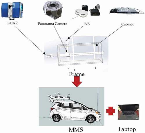
The MMS in this paper, which is integrated by POS LV 220 inertial navigation system produced by APPLANIX Company and Trimble GPS composed in a tightly coupled approach, FARO X130 3D scanner, PHITITANS panorama camera of TECHE Company and high-performance notebook computer. The INS and 3D LiDAR scanner specifications are shown in Tables 1 and 2, respectively.

Table 1. INS parameters (Applanix 2002)

Items	Parameters
IMU highest data update rate	200 Hz
plane accuracy	0.020 m
height accuracy	0.050 m
roll and pitch angle	0.015°
path angle	0.025°

Table 2. 3D LiDAR scanner parameters (Faro 2014)

Items	Parameters
scanning range	level 360°, vertical 360°
scanning distance	0.6 m – 330 m
maximum resolution	level: 0.009°, vertical: 0.009°
scanning speed	976,000 points/s
measure error	±2 mm
wavelength	1550 nm
environmental parameters	working temperature:5–40°C, working humidity: no condensation

As an integrated system, the precision of MMS is affected by various factors, which are categorized as boresight calibration error and component error (Xu 2016; Guo et al. 2017; Guo et al. 2021). The component error is mainly the accuracy error of each sensor, including scanner measurement error, GNSS positioning error, camera internal parameter calibration error, et al. (Guo and Zhou 2016), and the calibration method for a single sensor is relatively mature. The boresight calibration error is the position and angle deviation between sensors, such as the deviation between the scanner and frame coordinate system and the deviation between the camera and frame coordinate system, that is, the distance and angle deviation between sensor coordinate system and frame coordinate system (Puente et al. 2013; Shen et al. 2019; Jiao et al. 2011; Chan, Lichti, and Glennie 2013). In order to solve the problem of boresight calibration error, this paper starts from the positional and angular relationships between the scanner and the frame, establishes calibration field to calibrate MMS, and then uses various means to evaluate the accuracy of calibrated MMS.

In this paper, we propose a novel calibration method with error correction based on global coordinates. First, close-range photogrammetry technology is used to generate the point cloud model of the MMS system. In the scanner coordinate system, the physical characteristics of each sensor are used to calculate the initial transformation parameters of the scanner relative to the frame coordinate system. The MMS system studied in this paper uses the inertial navigation coordinate system as the frame coordinate system; that is, the deviation between the scanner and INS is obtained. Based on the initial value, error corrections are introduced, and an error correction model is constructed. The plane, sphere and other features in the high-precision calibration field measured in conjunction with IGS station are used for iterative calculation of correction adjustment, and the error corrections are solved. The obtained error corrections are combined with the initial value, thus obtaining the placement parameters of the scanner. Finally, the absolute accuracy and relative accuracy are analyzed. Besides, unlike other methods, it is shown that our proposed calibration method could improve the quality of the MMS point cloud significantly. Under the condition of low precision sensors, the absolute accuracy and relative accuracy could achieve a comparatively superior precision.

2. Calibration method

2.1. Overview methodology

Sensor calibration mainly includes feature point adjustment back-calculation, feature surface fitting solution, round-trip vertical wall surface solution and other methods (Yao, Wang and Sun 2016). Some scholars used a large number of point pairs to carry out optimal parameter settlement according to the spatial relationship between a large number of control points and their corresponding point clouds in the calibration field (Meng et al. 2014). Besides, Hu (2011) applied surface features to carry out final parameter determination and establish error equations according to laser point clouds with errors and plane equations, carry out correction iteration, and then eliminate the influence of errors. Different from the above, Yan et al. (2015) and Tian et al. (2014) used the coincidence of round-trip data to solve the angle deviation through round-trip observation of the same wall surface, thus realizing the calibration of parameters.

In the calibration of other integrated systems based on LiDAR, Stenz et al. (2017) used backward modeling of the uncertainty based on point clouds to complete the calibration of a TLS-based multi-sensor-system. Furthermore, Hong et al. (2017) proposed a method that through TLS generates point cloud to extract the point features for MMS calibration, and the precision of the boresight and lever-arm could be achieved by 0.1 degrees and 10 mm. Mishra, Pandey, and Saripalli (2020) presented a method, which uses the data collected by flat plates placed in different postures in the common field of view of LiDAR and camera, then a function model is established according to geometric constraints, and the LiDAR-Camera system is calibrated using non-linear least squares. Chen et al. (2019) used a method based on the laser tracer multi-station measurement system to calibrate the angular positioning deviation of a high-precision rotary table; according to their experimental results, the angular positioning deviation of the high-precision rotary table was as low as ±0.9”, and the error of the calibration method was ±0.4”.

In the aspect of the precision evaluation of MMS, Xu et al. (2019) completed the accuracy evaluation by establishing a permanent calibration field. They measured the absolute plane accuracy of 0.021 m, the absolute elevation accuracy of 0.023 m, and the relative accuracy of 0.015 m. Xu (2016) achieved good data accuracy after calibration, but the calibration field he established used more than hundreds of feature points, and the MMS he used was equipped with higher precision measurement sensors, which requires higher time and money costs. Similarly, Fan et al. (2019) also used the method that establishes a permanent calibration field to evaluate the accuracy of MMS. They measured the absolute X-direction accuracy of 0.192 m, the absolute Y-direction accuracy of 0.199 m, the absolute Z-direction accuracy of 0.221 m, and the relative accuracy of 0.039 m. Furthermore, Gizem and Cevdet (2019) measured billboards through mobile LiDAR and digital photogrammetry technology, respectively. Though they completed the measurement of billboards with mobile LiDAR quickly, the accuracy was between 1 and 1.5 m.

However, the calibration mentioned above method for the multi-sensors system has some defects. For example, some methods need to deploy too many control points (Shi et al. 2018; Meng et al. 2014; Fan et al. 2019), which takes a long time and cannot meet the requirements of fast and efficient calibration. Other methods calibrate the multisensor system by combining LiDAR point cloud and plane to establish error equations (Hu 2011), which do not take into account the loss of precision in plane feature fitting. Some other methods, according to the coincidence of the returned data to calibrate the system (Yan et al. 2015; Tian et al. 2014). Unfortunately, these methods do not take into account that the round-trip data of the mobile mapping system will have certain deviation due to the bumpy and moving track of the vehicle, which will lose the calibration accuracy. Also, at present, many calibration methods have not systematically evaluated the precision of the calibrated system (Stenz 2017; Mishra, Pandey, and Saripalli 2020), which makes the precision of the system, not convincing.

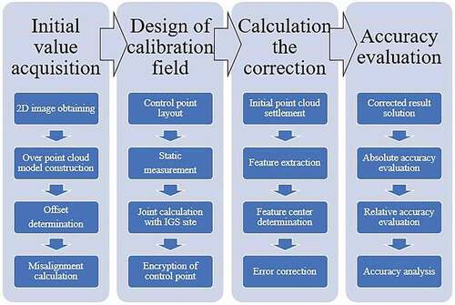
According to the calibration method of introducing error correction based on the initial value, the overall technical route is set as shown in Figure 2. First, the initial values of offset and misalignment are solved by the geometric relationship of sensors according to the overall point cloud model generated by image, and the MMS point cloud data calculated for the first time depends on this parameter. Then, the center coordinates of feature mark points are extracted in the point cloud calculated based on the initial value by the high-precision calibration field measured in conjunction with the IGS station. Then, relying on the feature points and their known coordinates to carry out the inverse calculation of the misalignment correction, the obtained error correction is brought into the coarse value, the MMS point cloud is recalculated by the calibrated parameters. Finally, the absolute accuracy of the point cloud obtained by MMS is verified according to the coordinate values, and the rationality of the method is proved by verifying the relative relationship between the ground object distances inside the point cloud.

Figure 2. Technical Roadmap: It is mainly divided into four steps: Firstly, obtaining the initial calibration value; Secondly, establishing the calibration field; Thirdly, calculating the correction; Finally, evaluating the accuracy

2.2. Obtaining the initial value of calibration

The initial value of calibration includes offset and misalignment. The methods for obtaining the initial value of calibration for offset can be divided into direct method and indirect method. The direct method mainly uses measuring tools such as a ruler to measure the relative relationship between each equipment directly. Although this method is simple to operate, it has a large human error and low precision. The indirect method mainly uses high-precision total station and other equipment to measure the geometric corners of sensors by setting up free stations and performs joint calculation with known sensor sizes and orientations. Compared with direct method, this method has greatly improved accuracy. Based on the characteristics of the MMS, this study propose a method to obtain the initial calibration value of the MMS by using the close-range photogrammetry technology. First, the close-range photogrammetry is used to obtain the 2D image of the MMS. Then, based on the SFM, fitting the 2D image obtained in the previous step into a 3D point cloud model (Shao, Chen, and Liu 2015; Chen and Shao 2013; Chen et al. 2013a, 2013b). Finally, the relative position relationship and relative posture of each device are solved by using mathematical models such as estimation regression model.

2.2.1. Accuracy comparison between close-range photogrammetry and total station

In order to verify the accuracy of the close-range photogrammetry, this paper uses the Leica TS30 total station to measure the coordinates of some points on MMS as the control group and calculate the RMSE of the two measurement methods, the technical parameters of Leica TS30 are shown in Table 3.

Table 3. The technical parameters of Leica TS30 (Leica 2009)

Items	Parameters
accuracy Hz and V	0.5”
display resolution	0.01”
method	absolute, continuous, diametrical
distance measurement (non-prism/any surface)	range:1.5 m to 1200 m; accuracy/measurement time: 2 mm+2ppm (typical 3–6s, max 12s)

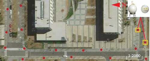
First, it arranges a large number of reflectors around the MMS, observing the center point of the reflector via Leica TS30, recording its coordinates and dividing all points into two groups: the control points and check points, the layout of reflectors is shown in Figure 3.

Figure 3. The layout of reflectors around MMS: A total of 27 reflectors are pasted on the MMS, among them, the red box is the verification point, and the yellow box is the control point

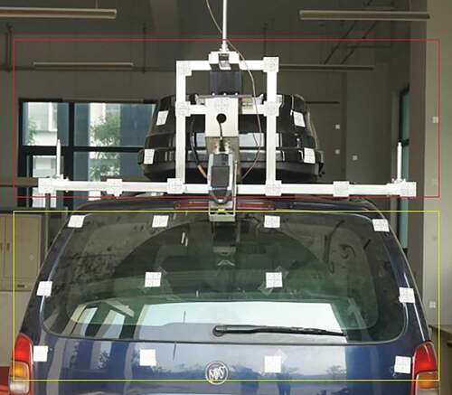
The accuracy of close-range photogrammetry can be analyzed by comparing the coordinates of the reflector’s center in the point cloud with the actual coordinates measured by the total station.

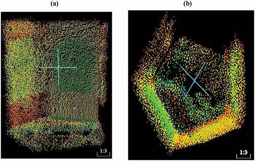
Second, SONY ILCE-7 R camera after calibration is used to obtain the 2D image of the MMS. In the experiment, the camera was placed on a half circle with a radius of 2 m, taking the MMS as the center of the circle. The shooting height is adjusted three times, corresponding to the bottom, middle and top of the MMS, respectively. After completing the photo shooting, using the Agisoft PhotoScan to process the image, importing control group as ground-control points. The 2D image obtained by close-range photogrammetry and the finally generated point cloud model of MMS are shown in Figure 4:

Figure 4. 2D image and point cloud model of MMS: (a) The 2D image of MMS is taken by digital camera, which can be used to generate refined 3D point clouds. (b) The point cloud model of MMS generated by 2D image, that could well reflect the spatial relationship of each sensor in MMS

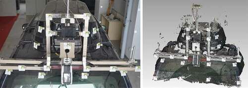
Finally, after the point cloud is generated, import it into Geomagic software, using the measurement function to measure the reflector’s center coordinates, the check points’ coordinates, as shown in Table 4. The total RMSE is 1.2 mm, which proves the method that using close-range photogrammetry to obtain MMS three-dimensional model has high precision. To some extent, it is feasible.

Table 4. The coordinates of verification points

Total station data			Point cloud data			Error
X/m	Y/m	Z/m	X/m	Y/m	Z/m	X/m	Y/m	Z/m
−0.0554	7.3423	1.9366	−0.0553	7.3423	1.9368	−0.0001	0.0000	−0.0002
0.0302	7.1583	1.9627	0.0304	7.1585	1.9628	−0.0002	−0.0002	−0.0001
0.1746	6.8805	1.9552	0.1746	6.8801	1.9556	0.0000	0.0004	−0.0004
0.3875	7.1212	1.9658	0.3879	7.1213	1.9664	−0.0004	−0.0001	−0.0006
0.5182	7.2810	1.9357	0.5190	7.2823	1.9358	−0.0008	−0.0013	−0.0001
−0.1089	7.2955	1.7718	−0.1091	7.2954	1.7716	0.0002	0.0001	0.0002
0.5601	7.2222	1.7824	0.5612	7.2229	1.7827	−0.0011	−0.0007	−0.0003
−0.2412	7.0598	1.6422	−0.2414	7.0598	1.6417	0.0002	0.0000	0.0005
0.3898	6.9913	1.6441	0.3899	6.9917	1.6443	−0.0001	−0.0004	−0.0002
0.6543	6.9686	1.6434	0.6548	6.9697	1.6432	−0.0005	−0.0011	0.0002
−0.4077	7.2381	1.4965	−0.4080	7.2383	1.4962	0.0003	−0.0002	0.0003
−0.0562	7.1243	1.5038	−0.0560	7.1251	1.5039	−0.0002	−0.0008	−0.0001
0.8378	7.0981	1.5012	0.8388	7.0990	1.5011	−0.0010	−0.0009	0.0001
−0.0810	6.9706	1.2779	−0.0802	6.9724	1.2761	−0.0008	−0.0018	0.0018
0.3922	6.9154	1.2868	0.3934	6.9166	1.2856	−0.0012	−0.0012	0.0012

2.2.2. Calculating the relative position relationship of each sensor

The coordinate origin of each sensor is inner to the sensor and cannot be directly picked up on the point cloud. In this paper, the position of the sensor origin in the point cloud coordinate system is indirectly obtained according to physical characteristics such as sensor surface information and shape.

Most of the MMS sensors are regular in shape, and the coordinate center can be solved by using a certain angular point coordinate of the sensor and an internally fixed size relation, specifically, (1) determining the angular point position; (2) determining the plane of the adjacent point cloud of the angular point, determining the plane equation; (3) solving the simultaneous Equation to solve the angular point coordinate; (4) determining the coordinate origin according to a fixed offset. For example, in inertial navigation, most IMUs are square cuboids. Plane fitting is carried out on three adjacent surfaces of IMU to obtain plane Equations. Three planes intersect at one point, and three plane equations are combined to obtain intersection coordinates, that is, coordinates of a certain corner point of IMU. Thus, the coordinates of the IMU center in the point cloud coordinate system are solved, the coordinates of each sensor center in the point cloud coordinate system are determined, and the distance offset of each sensor can be determined through a simple operation. Figure 5 is the center of the panorama camera.

Figure 5. Center of Panorama camera: a) Side view of panorama camera point cloud with the center of the cross as the center of panorama camera; b) Top view of panorama camera point cloud with the center of “X” being the center of panorama camera

For sensors with irregular shapes, such as GPS antennas. First, we measure the point coordinate at the connection between the antenna and the rigid frame according to the point cloud of MMS, and then add a fixed value (provided by the antenna manufacturer) to get the antenna center.

Since the coordinate axis of each equipment coordinate system is perpendicular to each plane, the angle deviation is indirectly measured by using the normal vector of the plane. Using this method, the normal vector of the plane perpendicular to the coordinate axis of each equipment independent coordinate system should be determined first, and the direction between the normal vector direction and the coordinate axis should be paid attention to avoid 180° difference. In the process of plane fitting, the plane normal vector is determined by the plane equation. The normal vectors are assumed to be $\vec{b}$, $\vec{d}$, and the angle θ are calculated as shown in Equations (1(1) $cos<\begin{array}{cc}\vec{b}& \vec{d}\end{array}>=\frac{\vec{b}\vec{d}}{|\vec{b}||\vec{d}|}$(1) ) and (2(2) $\theta ={cos}^{-1}\frac{\overrightarrow{b}\overrightarrow{d}}{|\overrightarrow{b}||\overrightarrow{d}|}$(2) ).

(1) $cos<\begin{array}{cc}\vec{b}& \vec{d}\end{array}>=\frac{\vec{b}\vec{d}}{|\vec{b}||\vec{d}|}$(1)

(2) $\theta ={cos}^{-1}\frac{\overrightarrow{b}\overrightarrow{d}}{|\overrightarrow{b}||\overrightarrow{d}|}$(2)

The above equation is used to calculate the angular difference of coordinate axes of different coordinate systems relative to the inertial navigation system coordinate system, to determine the angular deviation of each coordinate system in the inertial navigation coordinate system and obtain the attitude angle.

2.3. Error correction adjustment method

2.3.1. Design of the calibration field

The establishment of a high-precision calibration field is the premise for calculating accurate error correction and accuracy evaluation (Song, Gao and Li 2015). The calibration field is selected in an area with wide zone and less signal interference, and there are a certain number of curves and undulating sections in the field, which can better detect the influence brought by different environments and, at the same time, contain a large number of features and marking points, such as zebra crossing, streetlamp, traffic signal lamp, etc., providing reference for later precision evaluation (Zhang 2016).

After selecting the calibration site, the first-level control network is established. As the control reference of the calibration site, the first-level control network has high precision requirements. In order to ensure the precision of the control network, the relative positioning precision of the control points is improved by means of joint measurement with the surrounding IGS stations. IGS stations continuously track and observe all over the world and transmit data through special lines, networks or satellite communications to ensure that the daily observation data are automatically sent to the data center quickly, and provide various observation data, site coordinates, corresponding frames, epochs, station movement speed and other information to users around the world free of charge, which can meet our observation needs in time. There are four primary control points in this paper. After selecting points, GNSS receivers are used to carry out static observations on the control points for more than 2 hours. The static data, precise ephemeris and the station information of the surrounding IGS stations are subjected to joint baseline calculation and differential processing to obtain accurate control point coordinates. The joint calculation effect is shown in Figure 6.

Figure 6. Joint Settlement Based on IGS Stations: point distribution map, in this paper, six IGS control points are selected for adjustment; Results of adjustment Among them, points g03-g06 are the primary control points selected in this paper. From the Table, it can be seen that the adjustment errors are all less than 0.005 m

At the same time, different coordinate systems have different coordinate origins and reference ellipsoids. In order to avoid the error caused by coordinate transformation and to unify the coordinate systems, the coordinate of the calibration field in this paper adopts the same WGS-84 coordinate system as the MMS, and the plane coordinate is projected and calculated according to the 3-degree zone using Gaussian projection to ensure the accuracy of the calibration.

Based on the primary control network, it uses two kinds of feature points to encrypt the control network. In the range that MMS can observe, and have deployed a large number of special target balls, the schematic diagram and layout site of the target ball are shown in Figures 7 and 8.

Figure 7. Schematic diagram of target ball: 1) reflector 2) horizontal platform 3) horizontal bubble 4) spherical surface 5) support rod 6) base

Figure 8. Distribution of feature points: A total of 17 special target balls were set up as marking points and evenly distributed on both sides of the road in the calibration field. (As the red circle)

The target ball is placed on an annular base to make the target ball stationary; the top part of the target ball is equipped with a reflection sheet with a level bubble base. By adjusting the angle of the reflector to center the horizontal bubble, the center of the reflector and the center of the ball can be on the same vertical line so that the plane coordinate of the reflector is the center plane coordinate of the ball.

The study chooses some corner points of the facade of a building as feature points, such as corner points of windowsill and wall. The façade and some feature points of the selected building are shown in Figure 9.

Figure 9. Feature points of building facades: The feature points such as window corners (the red box) and wall corners (the yellow box) were selected in the facade of a building in the calibration site

When the feature points are laid out, observing them with Leica TS30 total station. For the special target ball feature points, using the total station to observe the center of the reflector on the upper part of the target ball for many times, the obtained plane coordinate is the real plane coordinate of the ball’s center, and the obtained elevation minus the inherent distance from the reflector’s center to the center of the ball is the real elevation of the ball’s center. For the feature points of building facades, use a total station to observe the corner points and record coordinates. During the measurement, we measured each feature point several times to reduce the influence of measurement error on the results, and the final average value is taken as the accurate calibration point coordinate.

2.3.2. Calibration algorithm

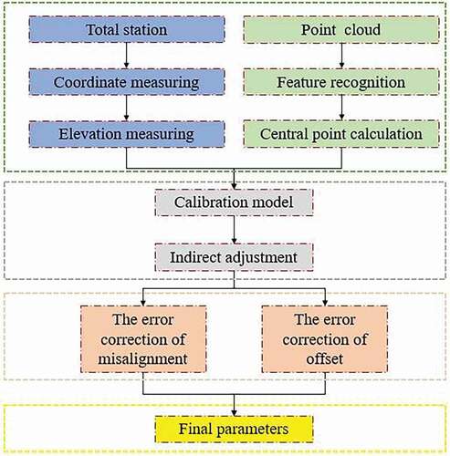
Based on obtaining initial values, error corrections are introduced, known control points and characteristic points are brought into the established error correction model, and the eccentric distance corrections and eccentric angle corrections of the laser scanner relative to IMU are reversely calculated by using the indirect adjustment method. The specific process is shown in Figure 10.

Figure 10. Flow chart of calibration: An error calibration model is established by combining the coordinates of control points measured by a high-precision total station and MMS, so as to calculate the offset and the misalignment error correction

In order to avoid the introduction of errors in the selection of feature points, a large number of target balls are arranged on the calibration site. The target balls are composed of a reflector and balls. There is a fixed gap between the center of the reflector and the center of the ball in the vertical direction. The total station measures the reflector and obtains the center coordinates according to the specific distance between the reflector and the center of the ball. The center coordinates of the point cloud cannot be directly measured. Therefore, the center coordinates of the point cloud must be determined before calibration. The center coordinates are solved through the inverse calculation of a large number of spherical points using Random Sampling Consensus algorithm (RANSAC) fitting algorithm, thus greatly improving the accuracy of data.

When using the indirect adjustment least square method, we need an accurate model to solve the error correction. An adjustment observation model is established according to the obtained initial value and error correction. The specific model is shown in Equation (3)(3) ${\left[\begin{array}{c}{X}_A\\ Y_A\\ Z_A\end{array}\right]}_{ECEF}=R_M\left[R_N\left[\mathrm{\Delta }{R}_0{R}_0\left[\begin{array}{c}{x}_I\\ y_I\\ z_I\end{array}\right]+\left[\begin{array}{c}{X}_{{ }_{LI}}\\ Y_{{ }_{LI}}\\ Z{\hspace{0.17em}}_{{ }_{LI}}\end{array}\right]+\left[\begin{array}{c}\mathrm{\Delta }{X}_0\\ \mathrm{\Delta }{Y}_0\\ \mathrm{\Delta }{Z}_0\end{array}\right]\right]\right]+{\left[\begin{array}{c}{X}_{\mathrm{g}\mathrm{p}\mathrm{s}}\\ Y_{\mathrm{g}\mathrm{p}\mathrm{s}}\\ Z_{\mathrm{g}\mathrm{p}\mathrm{s}}\end{array}\right]}_{ECEF}$(3) .

(3) ${\left[\begin{array}{c}{X}_A\\ Y_A\\ Z_A\end{array}\right]}_{ECEF}=R_M\left[R_N\left[\mathrm{\Delta }{R}_0{R}_0\left[\begin{array}{c}{x}_I\\ y_I\\ z_I\end{array}\right]+\left[\begin{array}{c}{X}_{{ }_{LI}}\\ Y_{{ }_{LI}}\\ Z{\hspace{0.17em}}_{{ }_{LI}}\end{array}\right]+\left[\begin{array}{c}\mathrm{\Delta }{X}_0\\ \mathrm{\Delta }{Y}_0\\ \mathrm{\Delta }{Z}_0\end{array}\right]\right]\right]+{\left[\begin{array}{c}{X}_{\mathrm{g}\mathrm{p}\mathrm{s}}\\ Y_{\mathrm{g}\mathrm{p}\mathrm{s}}\\ Z_{\mathrm{g}\mathrm{p}\mathrm{s}}\end{array}\right]}_{ECEF}$(3)

The model is a 3D coordinate system conversion model. Error corrections are introduced in the conversion process of the scanner and inertial navigation system. In Equation (3)(3) ${\left[\begin{array}{c}{X}_A\\ Y_A\\ Z_A\end{array}\right]}_{ECEF}=R_M\left[R_N\left[\mathrm{\Delta }{R}_0{R}_0\left[\begin{array}{c}{x}_I\\ y_I\\ z_I\end{array}\right]+\left[\begin{array}{c}{X}_{{ }_{LI}}\\ Y_{{ }_{LI}}\\ Z{\hspace{0.17em}}_{{ }_{LI}}\end{array}\right]+\left[\begin{array}{c}\mathrm{\Delta }{X}_0\\ \mathrm{\Delta }{Y}_0\\ \mathrm{\Delta }{Z}_0\end{array}\right]\right]\right]+{\left[\begin{array}{c}{X}_{\mathrm{g}\mathrm{p}\mathrm{s}}\\ Y_{\mathrm{g}\mathrm{p}\mathrm{s}}\\ Z_{\mathrm{g}\mathrm{p}\mathrm{s}}\end{array}\right]}_{ECEF}$(3) , the scanner coordinate of a certain point:$\left[x_I{y}_I{z}_I\right]$ . The initial values of the scanner coordinate system to inertial navigation coordinate system:$R_0$and ${\left[\begin{array}{ccc}{X}_{LI}& Y_{LI}& Z_{LI}\end{array}\right]}^{\mathrm{T}}$, which are known terms. Among them, $R_0$ is the rotation matrix formed by the initial values of angles, the initial values of translation amount:${\left[\begin{array}{ccc}{X}_{LI}& Y_{LI}& Z_{LI}\end{array}\right]}^{\mathrm{T}}$.$\mathrm{\Delta }{R}_0$ and $\left[\begin{array}{ccc}{\mathrm{\Delta }X}_0& {\mathrm{\Delta }Y}_0& {\mathrm{\Delta }Z}_0\end{array}\right]$are the error corrections introduced, the correction angle rotating around the X, Y and Z axis are. $\mathrm{\Delta }\alpha$, $\mathrm{\Delta }\beta$, $\mathrm{\Delta }\chi$, respectively. $\mathrm{\Delta }{R}_0$ can be expressed as Equation (4)(4) $\mathrm{\Delta }{R}_0=\mathrm{\Delta }{R}_{\alpha 0}\cdot \mathrm{\Delta }{R}_{\beta 0}\cdot \mathrm{\Delta }{R}_{\chi 0}$(4) .

(4) $\mathrm{\Delta }{R}_0=\mathrm{\Delta }{R}_{\alpha 0}\cdot \mathrm{\Delta }{R}_{\beta 0}\cdot \mathrm{\Delta }{R}_{\chi 0}$(4)

The specific matrix form is expressed as Equations (5(5) $\mathrm{\Delta }{R}_{\alpha 0}=\left[\begin{array}{ccc}1& 0& 0\\ 0& cos(\mathrm{\Delta }\alpha )& -sin(\mathrm{\Delta }\alpha )\\ 0& sin(\mathrm{\Delta }\alpha )& cos(\mathrm{\Delta }\alpha )\end{array}\right]$(5) ), (6(6) $\mathrm{\Delta }{R}_{\beta 0}=\left[\begin{array}{ccc}cos(\mathrm{\Delta }\beta )& 0& sin(\mathrm{\Delta }\beta )\\ 0& 1& 0\\ -sin(\mathrm{\Delta }\beta )& 0& cos(\mathrm{\Delta }\beta )\end{array}\right]$(6) ) and (7(7) $\mathrm{\Delta }{R}_{\chi 0}=\left[\begin{array}{ccc}cos(\mathrm{\Delta }\chi )& sin(\mathrm{\Delta }\chi )& 0\\ -sin(\mathrm{\Delta }\chi )& cos(\mathrm{\Delta }\chi )& 0\\ 0& 0& 1\end{array}\right]$(7) ).

(5) $\mathrm{\Delta }{R}_{\alpha 0}=\left[\begin{array}{ccc}1& 0& 0\\ 0& cos(\mathrm{\Delta }\alpha )& -sin(\mathrm{\Delta }\alpha )\\ 0& sin(\mathrm{\Delta }\alpha )& cos(\mathrm{\Delta }\alpha )\end{array}\right]$(5)

(6) $\mathrm{\Delta }{R}_{\beta 0}=\left[\begin{array}{ccc}cos(\mathrm{\Delta }\beta )& 0& sin(\mathrm{\Delta }\beta )\\ 0& 1& 0\\ -sin(\mathrm{\Delta }\beta )& 0& cos(\mathrm{\Delta }\beta )\end{array}\right]$(6)

(7) $\mathrm{\Delta }{R}_{\chi 0}=\left[\begin{array}{ccc}cos(\mathrm{\Delta }\chi )& sin(\mathrm{\Delta }\chi )& 0\\ -sin(\mathrm{\Delta }\chi )& cos(\mathrm{\Delta }\chi )& 0\\ 0& 0& 1\end{array}\right]$(7)

$R_N$ is the rotation matrix from the inertial navigation coordinate system to the local horizontal coordinate system. The local horizontal coordinate system is a station center coordinate system. The origin is the same as the origin of the inertial navigation coordinate system to avoid the drift of the coordinate origin. The angle transformation of $R_N$ is related to the installation and driving route of the inertial navigation system. The angle value can be calculated through the understanding of the inertial navigation system, and is also composed of $R_r{R}_p{R}_h$. $R_M$ and ${\left[\begin{array}{ccc}{X}_{\mathrm{g}\mathrm{p}\mathrm{s}}& Y_{\mathrm{g}\mathrm{p}\mathrm{s}}& Z_{\mathrm{g}\mathrm{p}\mathrm{s}}\end{array}\right]}^{\mathrm{T}}$are rotation and translation matrices from local horizontal coordinates to WGS-84, and $R_M$ can be expressed as Equation (8)(8) $\mathrm{\Delta }{R}_{\chi 0}=\left[\begin{array}{ccc}cos(\mathrm{\Delta }\chi )& sin(\mathrm{\Delta }\chi )& 0\\ -sin(\mathrm{\Delta }\chi )& cos(\mathrm{\Delta }\chi )& 0\\ 0& 0& 1\end{array}\right]$(8) .

(8) $\mathrm{\Delta }{R}_{\chi 0}=\left[\begin{array}{ccc}cos(\mathrm{\Delta }\chi )& sin(\mathrm{\Delta }\chi )& 0\\ -sin(\mathrm{\Delta }\chi )& cos(\mathrm{\Delta }\chi )& 0\\ 0& 0& 1\end{array}\right]$(8)

Under the condition that the local horizontal coordinate origin and the earth longitude and latitude (B,L) are known, according to the model, the error correction is established to linearize the error equation, the matrix form as Equation (9)(9) $V=BX-L$(9) .

(9) $V=BX-L$(9)

According to the principle of least squares, the Equation is calculated as Equation (10)(10) $B^{\mathrm{T}}PBX=B^{\mathrm{T}}PL$(10) .

(10) $B^{\mathrm{T}}PBX=B^{\mathrm{T}}PL$(10)

P is the weight matrix, plugging the calculated value into the error equation to carry out iterative calculation until the correction value is less than a certain threshold value so that the corrections $\mathrm{\Delta }\alpha$, $\mathrm{\Delta }\beta$, $\mathrm{\Delta }\chi$, $\mathrm{\Delta }{X}_0$, $\mathrm{\Delta }{Y}_0$, $\mathrm{\Delta }{Z}_0$ of the six parameters are solved.

3. Experimental design and result

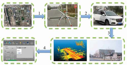
Clouds may affect GNSS signals on rainy days because part of the signal will be absorbed or scattered by cloud and rain (Bai 2014), the working environment of scanner and panorama camera also have a certain requirement on temperature and humidity. Starting and stopping the vehicle frequently will have a certain influence on the accuracy of the inertial navigation system. In order to gather higher data accuracy of MMS point clouds, experiments should be conducted when there are good weather and less traffic. After an on-the-spot investigation, the experimental site was selected as the highway inside and around a university campus in Beijing. The overall process of the experiment is shown in Figure 11.

Figure 11. The flow of the experiment: 1) planning a route: The first step in the data collection experiment. After setting the driving route, we can ensure that we can collect all kinds of point cloud data we need. 2) laying a base station: The role of the base station is to receive satellite signals and transmit them to the GNSS system of the MMS to ensure that the position information of the MMS can be updated in real time during data acquisition. 3) acquiring data: After completing the preparation for the experiment, we can begin to collect data. In the process of collecting data, we should as far as possible to avoid areas with weak satellite signals and drive at a constant speed. 4) preprocessing the data: This step includes coordinate transformation and registration of point cloud data, in this paper, we completed it through our own MMS data processing software

3.1. Data acquisition

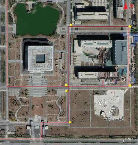
According to the experimental requirements, two known points 50 m apart with good satellite signals are selected to establish base stations in a school. Research is setting the acquisition mode to static acquisition. The acquisition time should exceed 2 hours, and the antenna must remain stationary during the collecting process. The experimental measurement area should be kept within 15 km from the base station, the location of the base station and the control points are shown in Figure 12. The main function of the base station is to provide GNSS observation values to the mobile station in real time and provide corrections to the vehicle GNSS receiver to improve the positioning accuracy of the MMS. After completing the acquisition, the high-precision driving trajectory can be obtained by fusion and calculation with IMU data of the MMS.

Figure 12. Location Map of Base Stations and Control Points: In the Figure, the red line is part of the driving route, the yellow circle is the GNSS base station (WGS84), and the yellow Pentagram is the control point

After confirming that the vehicle and equipment are connected normally, start the system and drive the vehicle to an open area to ensure that good GNSS signals are received. Let the vehicle stand for 6–8 min, then start the vehicle and go around for 5–10 min. The purpose is to initialize IMU to ensure the accuracy of inertial navigation data and point cloud data.

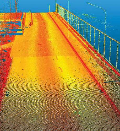
After completing the initialization of the MMS, the acquisition mode shall be preset, and the driving shall be smooth and uniform as far as possible according to the preplanned route. If the driving is to areas with dense buildings or large occlusion, the accuracy of the data shall be accelerated by preventing the GNSS signal from losing lock for too long. The collected point cloud data is shown in Figure 13.

Figure 13. The point clouds collected by the MMS

After collecting the data, drive the vehicle to an open area and stop data collection, letting the vehicle stand for 6–8 min. Check for data loss, and if so, judge whether to carry out secondary collection according to the actual situation. If the data collection is correct, export the collected data and shut down the system.

3.2. Data processing and results

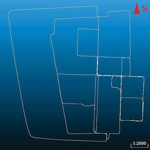
Import the collected GNSS data and INS data into the POSPac software for resolving. After the calculation is completed, the txt format driving track file as shown in Figure 14 will be obtained. The solution of the driving trajectory is the basis of the next point cloud data calculation, and also provides an important reference for finding control points in the MMS point cloud.

Figure 14. Driving track: Driving trajectory is the basis of data fusion calculation. Combining trajectory with planned driving route analysis can quickly find the point cloud area where the feature points are located (WGS84)

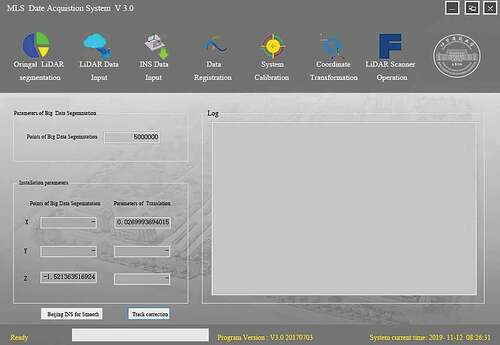
After the GNSS and IMU data are solved, using the self-developed data processing software, solve the MMS point cloud data. The software interface is shown in Figure 15.

Figure 15. Point cloud solution software: The self-developed MMS processing software using C# language. Through this software, the scanner can be operated during the working process of the MMS, and the data can be pre-processed such as registration and coordinate transformation after data acquisition is completed

4. Discussion

After data processing, we evaluated the absolute accuracy and relative accuracy of MMS. For absolute accuracy, this paper uses a total station to measure the spherical center coordinates of special target balls and compare the spherical center coordinates in the point cloud of MMS to evaluate the absolute accuracy. For the relative accuracy, it uses FARO X130 TLS (precision is 2 mm) and tape (precision is mm-level) to measure the size of some ground objects, respectively, and compare with the size in the MMS point cloud to evaluate the relative accuracy. In addition, it also uses the Geomagic software to analyze the relative accuracy.

4.1. Evaluation of absolute accuracy

The absolute accuracy of the MMS point cloud is the error between the coordinates of the control point scanned by the MMS and the real coordinates of the control point. This paper takes RMSE as the index of accuracy. The RMSE of absolute accuracy is analyzed according to Equation (11)(11) $\left.\begin{array}{c}{\sigma }_p=\pm \sqrt{\sum _{i=1}^n{\left(x_i-x_{in}\right)}^2+{\left(y_i-y_{in}\right)}^2/n}\\ {\sigma }_h=\pm \sqrt{\sum _{i=1}^n{\left(h_i-h_{in}\right)}^2/n}\end{array}\right\}$(11) .

(11) $\left.\begin{array}{c}{\sigma }_p=\pm \sqrt{\sum _{i=1}^n{\left(x_i-x_{in}\right)}^2+{\left(y_i-y_{in}\right)}^2/n}\\ {\sigma }_h=\pm \sqrt{\sum _{i=1}^n{\left(h_i-h_{in}\right)}^2/n}\end{array}\right\}$(11)

where $\left(\begin{array}{ccc}{x}_i& y_i& h_i\end{array}\right)$ represents the coordinates of the control points in the vehicle-mounted point cloud, and $\left(\begin{array}{ccc}{x}_{in}& y_{in}& h_{in}\end{array}\right)$ represents the actual coordinates of the measured control points, ${\sigma }_p$ represents the absolute plane accuracy, and ${\sigma }_h$ is the absolute elevation accuracy.

4.1.1. Absolute accuracy of point cloud before calibration

This paper uses a special target ball to calculate the characteristic points to analyze the absolute accuracy, the layout site of the target ball is shown in Figure 16. Using Leica TS30 total station, observe the reflector’s center on the top part of the target ball for many times and record the coordinates. In the point cloud data, this paper selects a large number of spherical points scanned by the MMS, uses RANSAC algorithm to fit the sphere, and calculates the spherical center coordinates of the target sphere, which can effectively avoid the error of manually selecting points and improve the accuracy of the data.

Figure 16. Layout of target balls: In the area that can be scanned by the MMS, a special target ball is arranged in a place with a wide field of vision and can be viewed back and forth, so that the measurement by the total station is more convenient and the measurement result is more accurate

In order to verify the reliability of the calibration method in this study, the coordinates of control points in the point cloud before calibration are compared with the actual coordinates of control points. The calibration method in this paper is judged by comparing the calibrated point cloud coordinates. The accuracy of point cloud before calibration is shown in Table 5.

Table 5. Absolute error of MMS before calibration

Point cloud data			Control point data			Error
X/m	Y/m	Z/m	X/m	Y/m	Z/m	X/m	Y/m	Z/m
****345.8727	***544.6109	33.7432	****345.8908	***544.6289	33.6606	0.0181	0.018	0.0826
****353.4933	***549.3423	33.5734	****353.468	***549.3607	33.4972	−0.0253	0.0184	0.0762
****390.0809	***497.4653	34.0346	****390.1221	***497.4174	33.9391	0.0412	−0.0479	0.0955
****409.1031	***489.9443	33.9529	****409.0690	***489.9869	34.0341	−0.0341	0.0426	−0.0812
****355.4514	***534.9364	35.0308	****355.4828	***534.9878	35.1079	0.0314	0.0514	−0.0771
****342.1816	***497.1055	34.8497	****342.2310	***497.1696	34.9309	0.0494	0.0641	−0.0812
****347.7673	***479.9609	33.3362	****347.7128	***479.9587	33.4200	−0.0545	−0.0022	−0.0838
****354.2386	***489.5274	33.1336	****354.1944	***489.5059	33.0523	−0.0442	−0.0215	0.0813
****521.8017	***499.7275	33.5868	****521.7503	***499.6963	33.677	−0.0514	−0.0312	−0.0902
****398.4699	***497.5656	35.306	****398.5473	***497.6118	35.2441	0.0774	0.0462	0.0619
****398.5941	***497.5684	35.1174	****398.6253	***497.6133	35.2087	0.0312	0.0449	−0.0913
****355.4367	***534.9193	34.9649	****355.4838	***534.9888	35.033	0.0471	0.0695	−0.0681
****342.1945	***497.1234	34.8535	****342.2311	***497.1868	34.9263	0.0366	0.0634	−0.0728

It can be seen from Table 5 that the error of X direction is roughly distributed between 0.02 m and 0.08 m, the error of Y direction is generally distributed between 0.02 m and 0.07 m, and the error of Z direction is approximately distributed between 0.06 m and 0.1 m. Using Equation (11)(11) $\left.\begin{array}{c}{\sigma }_p=\pm \sqrt{\sum _{i=1}^n{\left(x_i-x_{in}\right)}^2+{\left(y_i-y_{in}\right)}^2/n}\\ {\sigma }_h=\pm \sqrt{\sum _{i=1}^n{\left(h_i-h_{in}\right)}^2/n}\end{array}\right\}$(11) to calculate the RMSE of all measured feature points and the plane and elevation errors are estimated to be 0.054 m and 0.081 m separately.

4.1.2. Absolute accuracy of point cloud after calibration

The point cloud obtained after calibration is compared with the known control point data, the absolute and relative accuracy of the point cloud is compared and analyzed to verify the accuracy of the error correction of calibration. As shown in Table 6, it can be seen from the Table 6 that the error of the characteristic point in the X direction mainly distributed between 0.01 m and 0.05 m; The error of characteristic points in Y direction mainly distributed between 0.02 m and 0.05 m; The error of characteristic points in Z direction relatively large, mainly distributed between 0.02 m and 0.07 m. Using Equation (11)(11) $\left.\begin{array}{c}{\sigma }_p=\pm \sqrt{\sum _{i=1}^n{\left(x_i-x_{in}\right)}^2+{\left(y_i-y_{in}\right)}^2/n}\\ {\sigma }_h=\pm \sqrt{\sum _{i=1}^n{\left(h_i-h_{in}\right)}^2/n}\end{array}\right\}$(11) to calculate the RMSE of all measured feature points and the plane and elevation errors are calculated to be 0.043 m and 0.072 m separately.

Table 6. Absolute error of MMS before calibration

Point cloud data			Control point data			error
X/m	Y/m	Z/m	X/m	Y/m	Z/m	X/m	Y/m	Z/m
****345.9004	***544.6300	33.7213	****345.8908	***544.6289	33.6606	0.0096	0.0011	0.0607
****353.4652	***549.3609	33.5567	****353.4680	***549.3607	33.4972	−0.0028	0.0003	0.0594
****390.1475	***497.3715	33.9644	****390.1221	***497.4174	33.9391	0.0254	−0.0458	0.0253
****409.0640	***489.9882	33.9708	****409.0690	***489.9869	34.0341	−0.0051	0.0012	−0.0633
****355.4919	***535.0281	35.0698	****355.4828	***534.9878	35.1079	0.0091	0.0403	−0.0381
****342.2727	***497.2100	34.8848	****342.2310	***497.1696	34.9309	0.0417	0.0404	−0.0461
****347.6771	***479.9579	33.3720	****347.7128	***479.9587	33.4200	−0.0356	−0.0008	−0.0480
****354.1639	***489.4761	33.0934	****354.1944	***489.5059	33.0523	−0.0305	−0.0298	0.0411
****521.7098	***499.6599	33.6109	****521.7503	***499.6963	33.6770	−0.0404	−0.0364	−0.0661
****398.5953	***497.6265	35.2962	****398.5473	***497.6118	35.2441	0.0480	0.0147	0.0521
****398.6503	***497.6257	35.1594	****398.6253	***497.6133	35.2087	0.0250	0.0124	−0.0493
****355.4946	***535.0211	34.9810	****355.4838	***534.9888	35.0330	0.0108	0.0323	−0.0520
****342.2404	***497.2340	34.9075	****342.2311	***497.1868	34.9263	0.0093	0.0472	−0.0188

Table 7 shows the initial calibration value, the transformation parameters calibrated by the method in this paper and the RMSE of the corresponding control points. In Table 7, a, b and c represent three distance parameters, and α, β and γ represent three angle parameters.

Table 7. Absolute error of MMS after calibration

Items	Initial Parameters	Final Parameters
a	0.02741	0.02699
b	0.34817	0.32240
c	0.16007	0.15389
α	−30	−27.59452
β	180	−180.48123
γ	0	−1.52136
RMSE of control points		Plane: 0.043 m Elevation: 0.072 m

4.1.3. Accuracy analysis before and after calibration

By comparing the point clouds before and after calibration, it can be found that the method proposed in this paper can effectively achieve the MMS calibration, and the absolute accuracy of plane and elevation of the point cloud is improved by 0.011 m and 0.009 m, respectively, after calibration. The comparison diagram of a point cloud before and after calibration is shown in Figure 17.

Figure 17. Comparison diagram of a building’s point cloud before and after calibration (a) Front view of a building before and after calibration; (b) Top view of a building before and after calibration (In the above figures, the green point cloud is the point cloud data before calibration, and the white point cloud is the point cloud data after calibration)

4.2. Evaluation of relative accuracy

The relative accuracy of MMS refers to the comparison between the attributes of each object itself, such as the diameter of trees, the height of roadblocks, etc., and the attributes of the object in the MMS point cloud. The RMSE of relative accuracy is calculated according to Equation (12)(12) ${\sigma }_L=\pm \sqrt{\sum _{i=1}^n{\left(L_i-L_{in}\right)}^2/n}$(12) :

(12) ${\sigma }_L=\pm \sqrt{\sum _{i=1}^n{\left(L_i-L_{in}\right)}^2/n}$(12)

where L_i represents the value of the ground object in the point cloud, and L_in represents the actual value of the ground object, which ${\sigma }_L$ is the relative accuracy.

4.2.1. Compare with TLS point cloud to evaluate the relative accuracy

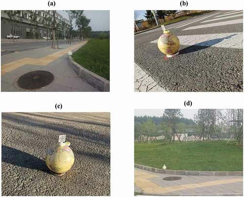
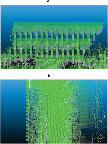
According to the actual situation, windowsill, guard room and garbage bin are selected as evaluation objects in this paper. TLS scans the above-ground objects. The height and width of the evaluation object in the TLS point cloud and MMS point cloud are measured, respectively, by CloudCompare point cloud processing software. Part of the point cloud data acquired by the TLS and MMS are shown in Figure 18.

Figure 18. Partial point cloud data on and from stations: (a) guard room data obtained by TLS; (b) windowsill data obtained by TLS; (c) guard room data obtained by MMS; (d) windowsill data obtained by MMS

Through multiple measurements and averaging, the data of each evaluation object are shown in Table 8. Using Equation 13 to calculate the TLS&MMS point cloud error, the relative accuracy of the MMS is 0.017 m eventually.

Table 8. Data of TLS control group

Object	TLS/m	MMS/m	Error/m
window	1.705	1.722	−0.017
guard room height	3.361	3.391	−0.03
guard room width	2.552	2.563	−0.011
trash can height	0.927	0.941	−0.014
trash can width	0.798	0.799	−0.001

4.2.2. Using tape to evaluate the relative accuracy

The study selects a number of street trees, lamps and stone piers for outdoor measurement and record these data as true values, Figure 19 is a partial data collection site.

Figure 19. Outdoor tape measurement: (a) the street tree diameter measurement site; (b) the stone pier height measurement site; (c) the street lamp pole diameter measurement site

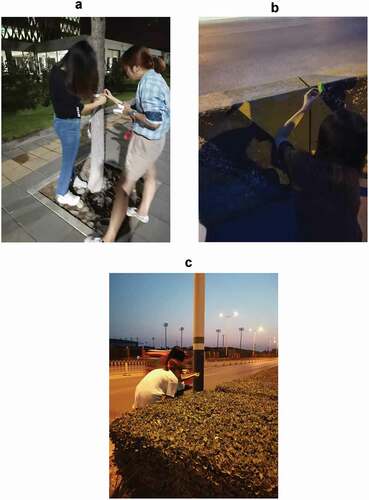
First, the study finds the point cloud model of the corresponding ground objects in MMS point cloud, then it fits the street trees and lampposts by CloudCompare point cloud processing software to get their diameters, and, finally, it measures the height of stone piers from bottom to top by ranging function. The obtained data are shown in Table 9, and the relative accuracy of the point cloud calculated by Equation (12)(12) ${\sigma }_L=\pm \sqrt{\sum _{i=1}^n{\left(L_i-L_{in}\right)}^2/n}$(12) is 0.011 m.

Table 9. Data of tape control group

Object	Tape/m	MMS/m	Error/m
tree1	0.203	0.226	−0.023
tree 2	0.15	0.144	0.006
tree 3	0.156	0.155	0.001
tree 4	0.158	0.148	0.01
tree 5	0.178	0.188	−0.01
tree 6	0.123	0.128	−0.005
tree 7	0.149	0.15	−0.001
tree 8	0.132	0.136	−0.004
tree 9	0.165	0.158	0.007
tree 10	0.143	0.154	−0.011
lamp1	0.157	0.136	0.021
lamp2	0.185	0.191	−0.006
stone pier1	0.845	0.836	0.009
stone pier2	0.847	0.85	−0.003

4.2.3. Through Geomagic software 3D analysis evaluate relative accuracy

This paper also analyzes the relative accuracy of the MMS through the 3D analysis between the TLS point cloud and the MMS point cloud. The 3D analysis is a function of Geomagic software for analyzing the deviation of two sets of point clouds. The basic idea is to carry out ICP iterative registration on two sets of point clouds first. Then, one group of point clouds is encapsulated into a 3D model as a reference grouping and another group of point clouds as a test group. Finally, calculate the distance between the point in the test group and the reference group’s model, and express the result in the form of a chromatogram. In this paper, the TLS point cloud is encapsulated into the 3D model as a reference group and MMS point cloud as a test group.

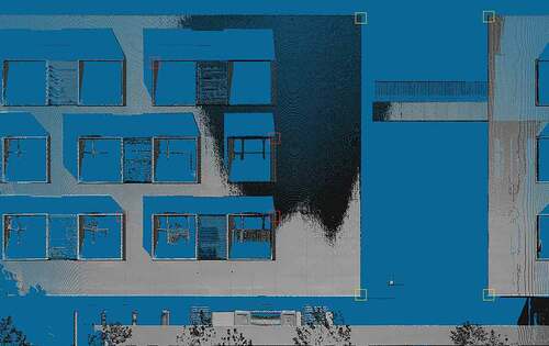
According to the actual situation of the scanning site, the front elevation of a school building is selected as the evaluation object. Due to limitations of the actual site and the instrument itself, the data of TLS and MMS point cloud cannot be completely coincident. In this paper, some non-coincident point clouds are deleted first, and then the model is compared by 3D analysis. The chromatogram of the 3D analysis of the TLS point cloud data model and the MMS point cloud data are shown in Figure 20.

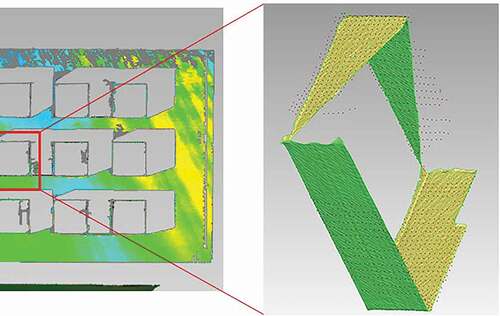
Figure 20. Chromatogram of point cloud TLS and MMS of a building: In this figure, the colored part is the overlapping part of the TLS point cloud data model and the MMS point cloud data, and the gray part did not participate in the comparison due to the lack of point cloud data

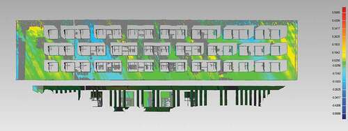
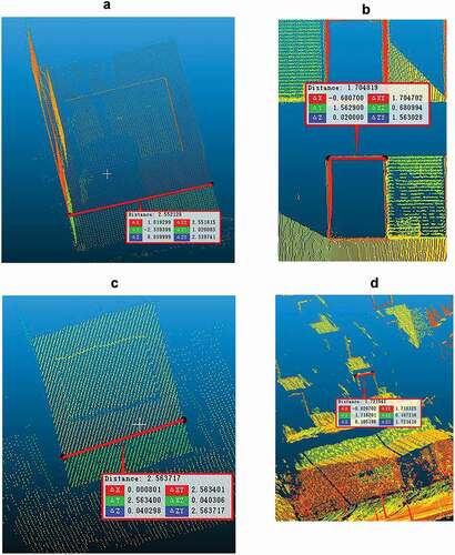
As we can see from Figure 20, most of the 3D models are green and blue, which indicates that the coincidence error is small. Because the model is too large to carry out accurate quantitative analysis, this paper selects a windowsill on the surface of the building to further explore the relative accuracy of the point clouds as shown in Figure 21.

Figure 21. Windowsill point cloud 3D model: In the Figure, yellow and green are the 3D models encapsulated by the point cloud data of the TLS, and red points are the point cloud data of the MMS

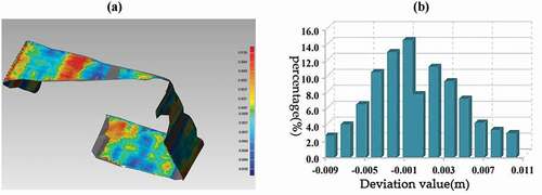
In order to make the obtained accuracy more reliable, the study only keeps a common part of the two sets of data, and then uses the Geomagic software to perform 3D analysis. The 3D model chromatogram and a deviation distribution graph are shown in Figure 22. The colors of the model in Figure 22(a) are mostly blue-green and orange-yellow as can be seen from the observation of the deviation distribution in Figure 22(b), the error is mainly distributed between −0.005 m and+0.005 m.

Figure 22. 3D analysis results of windowsill model: (a) 3D analysis chromatogram, tolerance is −0.01 m – 0.01 m, turquoise is more observed from the Figure, indicating that the overall deviation is smaller (b) overall deviation distribution diagram, deviation is approximately positive distribution, and most deviation is within 0.005 m

4.2.4. Analysis of the relative accuracy

To summarize, the relative accuracy measured by the above three methods are about 0.017 m, 0.011 m and approximately 0.005 m, respectively. There are some reasons for the inconsistent relative precisions:

1. TLS has high measurement accuracy but is affected by its resolution. The scanning accuracy is half of the distance between the two points measured by TLS. When scanning corner points, TLS may miss edge information, and the measurement accuracy will be lower. Moreover, when measuring the size of the object in the point cloud, the accuracy will be lost due to the point selection error.

2. The precision standard of tape is millimeter level, and the study uses the method of multiple measurements to take average value in this paper, which can effectively reduce the error in the measurement process.

3. The 3D analysis is an effective method to analyze the errors of two groups of the point cloud. The basic idea is to package a group of point cloud into a 3D model, and then compare another set of point cloud with the model to determine whether the two sets of data coincide. Before the 3D analysis in this paper, we deleted the missing data due to the scanning angle, etc. In this way, the loss of precision caused by missing data can be eliminated, thus making the evaluation result more accurate and reliable.

5. Conclusions

In this study, the MMS combining panorama camera, 3D LiDAR scanner, and GNSS/INS was developed, and the effect of the MMS calibration was proposed. The initial value of the relative relationship between sensors was solved by using the point cloud model data of MMS acquired by close-range photogrammetry. On this basis, error correction was introduced, and six error corrections were solved by using the established high-precision calibration field, and the MMS results were solved according to the final parameters of the introduced error correction.

Through our extensive stability analysis, the absolute and relative precisions of the calibrated MMS were evaluated:

The plane absolute precision and absolute elevation precisions of the MMS are 0.043 m and 0.072 m, respectively, and the relative precision could be achieved smaller than 0.02 m.

The main advantages of applying the method proposed in this paper to the MMS calibration problem are efficiency and precision. On the one hand, it is difficult to observe the reference coordinate system accurately by existing means. On the other hand, the traditional method to measure various parameters of each sensor is inaccurate and labor-intensive. In this regard, using the method in this study can significantly reduce the work time for the MMS calibration. Furthermore, we evaluated the accuracy of point cloud after calibration and introduced IGS, which not only ensures the reliability of the results but also prepares for the future MMS era without base station.

Research also has some deficiencies. For example, the method of generating MMS point cloud using digital images mainly depends on third-party software, and only the scanner is calibrated, but the panorama camera is not calibrated.

To sum up, the final data show that the calibration method in this paper can effectively reduce the accuracy loss of the sensor. Under the condition that the accuracy of a single measurement sensor is not high, the final acquired result data could be achieved with a better absolute and relative accuracy.

Data availability statement

The data that support the findings of this study are available from the corresponding author, [Jianghong Zhao], upon reasonable request.

Additional information

Funding

This research was funded by the National Natural Science Foundation of China [grant number 41971350 and 41571437]; Beijing Advanced Innovation Centre for Future Urban Design Project [grant number UDC2019031724]; Teacher Support Program for Pyramid Talent Training Project of Beijing University of Civil Engineering and Architecture [grant number JDJQ20200307]; State Key Laboratory of Geo-Information Engineering [grant number SKLGIE2019-Z-3-1]; Open Research Fund Program of LIESMARS [grant number 19E01]; National Key Research and Development Program of China [grant number 2019YFC1520100]. The Fundamental Research Funds for Beijing University of Civil Engineering and Architecture [grant number X18050].

Notes on contributors

Ming Guo

Ming Guo is a professor of Beijing University of Civil Engineering and Architecture. His main research fields are mobile mapping technology, 3D geographic information management and visualization, building health monitoring, and low altitude UAV mapping application technology.

Yuquan Zhou

Yuquan Zhou is currently pursuing the M.S. degree with Beijing University of Civil Engineering and Architecture. His current research interests include mobile LiDAR scanning and point cloud segmentation.

Jianghong Zhao

Jianghong Zhao is a professor and vice president of School of Surveying and Mapping and Urban Spatial Information, Beijing University of Civil Engineering and Architecture. Her main research fields are Deep Learning, application of Deep Neural Network in Point Cloud, and Processing and Visualization of 3D LiDAR Data.

Tengfei Zhou

Tengfei Zhou is currently pursuing the M.S. degree in photogrammetry and remote sensing with Beijing University of Civil Engineering and Architecture. He is interested in track correction of vehicle LiDAR scanning system, and processing of LiDAR point clouds data.

Bingnan Yan

Bingnan Yan is currently pursuing the M.S. degree in photogrammetry and remote sensing with the Beijing University of Civil Engineering and Architecture. She is interested in track correction of vehicle LiDAR scanning system, and 3D reconstruction of ancient buildings.

Xianfeng Huang

Xianfeng Huang is professor of LIESMARS, Wuhan University. His main research fields are laser scanning data processing photogrammetry & remote sensing digital culture heritage urban computing.

References

- Applanix. 2002. “POS-LV-Datasheet.” https://www.applanix.com/downloads/products/specs/POS-LV-Datasheet.pdf
- Bai, Y. 2014. Research on GNSS Spatial Signal Interference Evaluation and Suppression Method. Beijing: PhD diss., University of Chinese Academy of Sciences.
- Chan, T. O., D. D. Lichti, and C. L. Glennie. 2013. “Multi-feature Based Boresight Self-calibration of a Terrestrial Mobile Mapping System.” Isprs Journal of Photogrammetry & Remote Sensing 82: 112–124. (aug.). doi:https://doi.org/10.1016/j.isprsjprs.2013.04.005.
- Chen, H., B. Jiang, H. Lin, S. Zhang, Z. Shi, H. Song, and Y. Sun. 2019. “Calibration Method for Angular Positioning Deviation of a High-Precision Rotary Table Based on the Laser Tracer Multi-Station Measurement System.” Applied Sciences 9 (16): 3417. doi:https://doi.org/10.3390/app9163417.
- Chen, M., and Z. Shao. 2013. “Robust Affine-invariant Line Matching for High Resolution Remote Sensing Images.” Photogrammetric Engineering & Remote Sensing 79 (8): 753–760. doi:https://doi.org/10.14358/PERS.79.8.753.
- Chen, M., Z. Shao, C. Liu, and J. Liu. 2013b. “Scale and Rotation Robust Line-based Matching for High Resolution Images.” Optik - International Journal for Light and Electron Optics 124 (22): 5318–5322. doi:https://doi.org/10.1016/j.ijleo.2013.03.110.
- Chen, M., Z. Shao, D. Li, and J. Liu. 2013a. “Invariant Matching Method for Different Viewpoint Angle Images.” Applied Optics 52 (1): 96–104. doi:https://doi.org/10.1364/AO.52.000096.
- Craciun, D., A. Serna-Morales, J.-E. Deschaud, B. Marcotegui, and F. Goulette. 2014. “Scalable and Detail-Preserving Ground Surface Reconstruction from Large3D Point Clouds Acquired by Mobile Mapping Systems.” PCV (Photogrammetric Computer Vision) 73 – 80. doi:https://doi.org/10.5194/isprsarchives-XL-3-73-2014.
- Fan, D. L., S. Ma, H. Liu, Q. Tang, and S. Yang. 2019. “Construction of Calibration Field and Precision Evaluation for Vehicle Mobile Measurement System.” China Metal Bulletin 24 (6): 124–126.
- Faro.2014. “Faro X130 3D Datasheet.” http://www.faroasia.com/LaserScanner/cn
- Ghouaiel, N., and L. Sébastien. 2016. “Coupling Ground-level Panoramas and Aerial Imagery for Change Detection.” Geo-spatial Information Science 19 (3): 222–232. doi:https://doi.org/10.1080/10095020.2016.1244998.
- Guo, M., B. N. Yan, T. F. Zhou, D. Pan, and G. L. Wang. 2021. “Accurate Calibration of a Self-Developed Vehicle-Borne LiDAR Scanning System.” Journal of Sensors 2021 (4): 1–18. doi:https://doi.org/10.1155/2021/8816063.
- Guo, M., S. Dong, X. Sheng, C. Cheng, and D. Pan. 2017. “Research on calibration technology of vehicle laser scanning system.” 20173rd IEEE International Conference on Computer and Communications (ICCC). IEEE.
- Guo, M., G. L. Wang, C. Chen, and M. Huang. 2018. Design Principle and Implementation Method of Mobile Measurement System. Beijing: Science Press.
- Guo, M., and X. P. Zhou. 2016. The Technology of Mobile Geographic Information System, 15–30. Beijing: China Architecture & Building Press.
- Guo, M., Y. Q. Zhou, C. Chen, Z. J. Zhou, and K. C. Guo. 2020. “Design of Time Synchronization Device for Mobile LiDAR Measurement System Based on BeiDou Navigation Timing.” Infrared and Laser Engineering 49 (S2): 33–42. doi:https://doi.org/10.3788/IRLA20200362.
- Hollick, J., P. Helmholz, and D. Belton. 2016. “Non-parametric Belief Propagation for Mobile Mapping Sensor Fusion.” Geo-spatial Information Science 19 (3): 195–201. doi:https://doi.org/10.1080/10095020.2016.1235816.
- Hong, S., I. Park, J. Lee, K. Lim, Y. Choi, and H. G. Sohn. 2017. “Utilization of a Terrestrial Laser Scanner for the Calibration of Mobile Mapping Systems.” Sensors (Basel) 17 (3): 474. doi:https://doi.org/10.3390/s17030474. Published 2017 Feb 27.
- Hu, J. 2011. Research on Overall Calibration Method of Vehicle 3D Laser Moving Modeling System, 18–35. Beijing: Capital Normal University.
- Jiao H. W., S. Q. Qin, C. S. Hu, and X. S. Wang. 2011. “Research on the Coordinates Calibration of Pulse LiDAR and Camera.” Chinese Journal of Lasers 38 (1): 0108006. doi:https://doi.org/10.3788/CJL201138.0108006.
- Kurtca, G., and C. C. Aydin. 2019. “Evaluation of Metric Measurement Accuracy Comparison on Advertising Billboards Using Mobile LiDAR and Digital Photogrammetry Techniques.” Fresenius Environmental Bulletin 28 (10): 7151–7162.
- Leica.2009. “Leica TS30 Datasheet.” https://w3.leicageosystems.com/downloads123/zz/tps/ts30/brochuresdatasheet/ts30_technical_data_en.pdf
- Li, D., J. Shan, Z. Shao, X. Zhou, and Y. Yao. 2013. “Geomatics for Smart Cities - Concept, Key Techniques, and Applications.” Geo-spatial Information Science 16 (1): 13–24. doi:https://doi.org/10.1080/10095020.2013.772803.
- Li, Y., S. Takayuki, T. Satoh, and K. Tachibana. 2016. “Road Signs Detection and Recognition Utilizing Images and 3D Point Cloud Acquired by Mobile Mapping System.” ISPRS - International Archives of the Photogrammetry, Remote Sensing and Spatial Information Sciences XLI-B1: 669–673. doi:https://doi.org/10.5194/isprsarchives-XLI-B1-669-2016.
- Meng X. G., S. X. Hu, A. W. Zhang, Y. H. Duan, and X. Zhang. 2014. “A Self-Calibration Method for Bore-Sight Error of Ground-Based Mobile Mapping System.” Chinese Journal of Lasers 41 (11): 1108008. doi:https://doi.org/10.3788/CJL201441.1108008.
- Mishra, S., G. Pandey, and S. Saripalli 2020. “Extrinsic Calibration of a 3D-LIDAR and a Camera.” 31st IEEE Intelligent Vehicles Symposium October 20–23, 2020, Las Vegas, NV. doi: https://doi.org/10.1109/IV47402.2020.9304750.
- Pozo-Antonio, J. S., I. Puente, M. F. C. Pereira, and C. S. A. Rocha. 2019. “Quantification and Mapping of Deterioration Patterns on Granite Surfaces by Means of Mobile LiDAR Data.” Measurement 140: 227–236. doi:https://doi.org/10.1016/j.measurement.2019.03.066.
- Puente, I., H. González-Jorge, B. Riveiro, and P. Arias. 2013. “Accuracy Verification of the Lynx Mobile Mapper System.” Optics & Laser Technology 45: 578–586. doi:https://doi.org/10.1016/j.optlastec.2012.05.029.
- Sester, M. 2020. “Analysis of Mobility Data – A Focus on Mobile Mapping Systems.” Geo-spatial Information Science 23 (1): 68–74. doi:https://doi.org/10.1080/10095020.2020.1730713.
- Shams, A., W. A. Sarasua, A. Famili, W. J. Davis, J. H. Ogle, L. Cassule, and A. Mammadrahimli. 2018. “Highway Cross-Slope Measurement Using Mobile LiDAR.” Transportation Research Record 2672 (39): 88–97. doi:https://doi.org/10.1177/0361198118756371.
- Shao, Z., and J. Cai. 2018. “Remote Sensing Image Fusion With Deep Convolutional Neural Network.” IEEE Journal of Selected Topics in Applied Earth Observations and Remote Sensing 11 (5): 1656–1669. doi:https://doi.org/10.1109/JSTARS.2018.2805923.
- Shao, Z., L. Zhang, and L. Wang. 2017. “Stacked Sparse Autoencoder Modeling Using the Synergy of Airborne LiDAR and Satellite Optical and SAR Data to Map Forest Above-Ground Biomass.” IEEE Journal of Selected Topics in Applied Earth Observations & Remote Sensing 1–14. doi:https://doi.org/10.1109/JSTARS.2017.2748341.
- Shao, Z., M. Chen, and C. Liu. 2015. “Feature Matching for Illumination Variation Images.” Journal of Electronic Imaging 24 (3): 033011. doi:https://doi.org/10.1117/1.JEI.24.3.033011.
- Shao, Z., N. Yang, X. Xiao, L. Zhang, and Z. Peng. 2016. “A Multi-view Dense Point Cloud Generation Algorithm Based on Low-altitude Remote Sensing Images.” Remote Sensing 8 (5): 381. doi:https://doi.org/10.3390/rs8050381.
- Shao, Z., N. S. Sumari, A. Portnov, F. Ujoh, and P. J. Mandela. 2020. “Urban Sprawl and Its Impact on Sustainable Urban Development: A Combination of Remote Sensing and Social Media Data.” Geo-spatial Information Science, no. 3: 1–15. doi:https://doi.org/10.1080/10095020.2020.1787800.
- Shao, Z., W. Wu, and D. Li. 2021. “Spatio-temporal-spectral Observation Model for Urban Remote Sensing.” Geo-spatial Information Science 1–15. doi:https://doi.org/10.1080/10095020.2020.1864232.
- Shao, Z. F., and D. R. Li. 2011. “Image city sharing platform and its typical applications.” Science China 54(8):1738–1746. doi:https://doi.org/10.1007/s11432-011-4307-7.
- Shen, X., M. Guo, and S. Dong. 2018. “Research on Calibration Method of Vehicle Mapping System Based on Special Target.” DEStech Transactions on Computer Science and Engineering. doi:https://doi.org/10.12783/dtcse/csae2017/17534.
- Shen X. W., M. Guo, G. L. Wang, and R. M. Shi. 2019. “The Overall Calibration Method of the Mobile Mapping System.” Science of Surveying and Mapping, no. 5: 138–145.
- Shi R. M., G. N. Wei, M. Guo, and Y. Hao. 2018. “Calibration of the Mobile Measurement System Based on the Least Squares Method.” Geotechnical Investigation&Surveying 46 (2): 53–57.
- Song, Y., Z. G. Gao, and C. H. Li. 2015. “Discussion on Accuracy Test of Mobile Laser Measurement System.” Science of Surveying and Mapping 40 (9): 74–77. doi:https://doi.org/10.16251/j.cnki.1009-2307.2015.09.015.
- Stenz, U., J. Hartmann, J.-A. Paffenholz, and I. Neumann. 2017. “A Framework Based on Reference Data with Superordinate Accuracy for the Quality Analysis of Terrestrial Laser Scanning-Based Multi-Sensor-Systems.” Sensors 17 (8): 1886. doi:https://doi.org/10.3390/s17081886.
- Sun, H., L. Leilei, X. Ding, and B. Guo. 2016. “The Precise Multimode GNSS Positioning for UAV and Its Application in Large Scale Photogrammetry.” Geo-spatial Information Science 19 (3): 188–194. doi:https://doi.org/10.1080/10095020.2016.1234705.
- Tian X. R., L. J. Xu, T. Xu, and Q. Zhang. 2014. “Calibration of Installation Angles for Mobile LiDAR Scanner System.” Infrared and Laser Engineering 43 (10): 3292–3297.
- Xu, S. Z. 2016. Research on Calibration of Moving Modeling System for Land Vehicle and Its Accuracy Assessment, 79–85. Wuhan: Wuhan University.
- Xu S. Z., A. P. Fang, F. Yang, and Y. Li. 2019. “Point Clouds Accuracy Assessment Method of Mobile Mapping System for Land Vehicle.” Science of Surveying and Mapping 44 (6): 187–192. doi:https://doi.org/10.16251/j.cnki.1009-2307.2019.06.027.
- Yan, L., H. Li, C. J. Chen, and L. Cao. 2015. “A Calibration Method of Mobile Laser System without Control Points.” Geomatics and Information Science of Wuhan University 40 (8): 1018–1022. doi:https://doi.org/10.13203/j.whugis20130782.
- Yang, B., and J. Wang. 2016. “Mobile Mapping with Ubiquitous Point Clouds.” Geo-spatial Information Science 19 (3): 169–170. doi:https://doi.org/10.1080/10095020.2016.1244982.
- Yao L. B., Z. F. Wang, H. L. Sun, and H. L. Sun. 2016. “Design and Implementation of Vehicle Laser Scanner’s External Parameter Calibration.” Journal of Tongji University 44 (1): 161–166. doi:https://doi.org/10.11908/j.0253-374x.2016.01.024.
- Yoshimura, R., H. Date, S. Kanai, R. Honma, K. Oda, and T. Ikeda. 2016. “Automatic Registration of MLS Point Clouds and SfM Meshes of Urban Area.” Geo-spatial Information Science 19 (3): 171–181. doi:https://doi.org/10.1080/10095020.2016.1212517.
- Zhang, L. 2016. “Layout and Implementation of Calibration Filed for Vehicle Laser Measurement System.” Journal of Geomatics 40 (4): 87–90. doi:https://doi.org/10.14188/j.2095-6045.2016.04.020.
- Zhang, Y., and L. Yan. 2007. “Road Surface Modeling and Representation from Point Cloud Based on Fuzzy Clustering.” Geo-spatial Information Science 10 (4): 276–281. doi:https://doi.org/10.1007/s11806-007-0106-0.