Spatial-temporal modeling of initial COVID-19 diffusion: The cases of the Chinese Mainland and Conterminous United States

ABSTRACT

COVID-19 outbreaks in China in late December 2019, then in the United States (US) in early 2020. In the initial wave of diffusion, the virus respectively took 14 and 33 days to spread across the provinces/states in the Chinese mainland and the coterminous US, during which there are 43% and 70% zero entries in the space-time series for China and US respectively, indicating a zero-inflated count process. A logistic growth curve as a function of the number of days since the first case appeared in each of these countries accurately portrays the national aggregate per capita rates of infection for both. This paper presents two space-time model specifications, one based upon the generalized linear mixed model, and the other upon Moran eigenvector space-time filtering, to describe the spread of COVID-19 in the initial 19 and 58 days across the Chinese mainland and the coterminous US, respectively. Results from these case studies show both models shed new light on the role of spatial structures in COVID-19 diffusion, models that can forecast new cases in subsequent days. A principal finding is that describing the spatio-temporal diffusion of COVID-19 benefits from including a hierarchical structural component to supplement the commonly employed contagion component.

KEYWORDS:

• COVID-19
• contagion diffusion
• hierarchical diffusion
• moran eigenvector spatial-time filtering
• random effects

1. Introduction

Since the COVID-19 outbreaks in January 2020, researchers have rushed to understand the first-wave space-time dynamic of the disease, and to assess the effects of containment measurements. Classical analytical and numerical models in epidemiology were employed. Leung et al. (2020), for example, estimated the instantaneous reproduction number and the confirmed case-fatality risk of COVID-19 in major cities and provinces in China, followed by employing a Susceptible-Infectious-Recovered (SIR) model to assess the potential effects of relaxing containment measures after the first wave of infection. Fanelli and Piazza (2020) used SIR to conduct a similar analysis across China, Italy, and France. Both Danon et al. (2020) and Peixoto et al. (2020) adopted metapopulation models to describe and predict the spread of the disease from regions to regions across England and Wales, and Brazilian states of São Paulo and Rio de Janeiro. Meanwhile, spatial statistical models also were applied to understand the disease space-time dynamics. For example, Guliyev (2020) employed a spatial panel data model to tackle the issue of contagion diffusion within the context of China, identifying spatial effects pertaining to not only the spread of cases, but also deaths and recoveries. Giuliani et al. (2020) developed an endemic-epidemic multivariate time-series mixed-effects GLM for areal counts of the COVID-19 cases to describe and predict the space-time distribution of the disease across Italy. Briz-Redón and Serrano-Aroca (2020) adopted a Bayesian approach to analyze the effect of temperature on the accumulated COVID-19 cases, finding no evidence of associations between warmer weather and reduction of cases. These state-of-the-art modeling efforts contributed to our understanding of the space-time dynamics of the disease. They are, however, largely focused on contagion diffusion of the disease. Hierarchical diffusion, another dimension of disease dynamics, has not been explicitly addressed in these models.

Spatial diffusion theory maintains that disease diffusion almost always follows two proliferation pathways: contagion, spread channeled by contiguous spatial autocorrelation; and, hierarchical, spread jumping between distant places channeled by an ordered sequence of places, frequently an urban system (Hägerstrand 1953; Gould 1969; Cliff et al. 1981; Reyes et al. 2013). An omission of the hierarchical dimension is clearly a deficit, which presents an opportunity for enhancing the current modeling efforts and gaining better understanding of the COVID-19 space-time dynamics. Achieved improvement with this expanded conceptualization can be further assessed by setting the modeling context in two countries comparable in size, namely China, where early outbreaks occurred, and the United States (US), where the disease was rapidly spread across the country after its first appearance.

Therefore, the objective of the paper is two-fold: (1) to present a spatial analysis of the initial spread of COVID-19 across the Chinese mainland as well as across the coterminous US in terms of both contagion and hierarchical diffusion; and, (2) to compare the modeling results for the two countries. The core approach is to represent the spatio-temporal dynamics of COVID-19 cases with a Generalized Linear Mixed Model (GLMM), where either Moran Eigenvector Spatial Filtering (MESF) or Moran Eigenvector Spatial Temporal Filtering (MESTF) represents the random effects (Griffith, Chun, and Li 2019) included in a model specification. This semi-parametric approach has the advantage of conceptual clarity as spatial-temporal structural information can be directly incorporated in a GLMM without substantial alternation of the estimation algorithm.

In the subsequent sections, we present details about the specifications of two GLMM models, one with MESF and another with MESTF. The methodology section also presents model estimation and workflows as well as descriptions of the datasets, including the constructions of the hierarchical spatial weights matrices for both China and the US. We then report estimation results for the spatio-temporal diffusions across the two respective countries with two GLMM model specifications. The conclusion section discusses findings from this project as well as enumerates future research agenda items.

2. Methodology

The spatial statistical methodology of interest is twofold: (1) Generalized Linear Mixed Modeling (GLMM), which includes a Random Effects (RE) term; and, (2) Moran Eigenvector Space-Time Filtering (MESTF) coupled with a RE term. The time series part of a space-time series for each location furnishes repeated measures for estimating each time-invariant RE term in the two analyses summarized in this paper. For the Chinese mainland, the individual location-specific RE term values are indistinguishable from their Fixed Effects (FE) term counterparts, except for Xizang Autonomous Region, whose confidence intervals for both values include the other value. For the conterminous US, all 49 sets of values are indistinguishable. Consequently, especially after considering arguments in Frondel and Vance (2010), RE specifications were adopted for this paper.

2.1 Modeling Considerations

Moran Eigenvector Spatial Filtering (MESF) is one of the major methodological approaches to accounting for spatial structural information in regression modeling (Giuliani et al. 2020; Griffith, Chun, and Li 2019). Instead of estimating parameters based upon the auto-specified modified likelihood functions of spatial variables, MESF selects a subset of eigenvectors from the doubly centered Spatial Weights Matrix (SWM) of a given geographic landscape (partitioning or configuration) as covariates in conventional non-spatial regression models to filter spatial autocorrelation out of regression residuals; this filtering transfers the spatial effects to the intercept term, and renders residuals that mimic spatially independent ones. The resulting linear combination of the statistically significant eigenvectors forms an Eigenvector Spatial Filter (ESF) that accounts for spatial information in the model.

The mathematical foundation of MESF is matrix eigen-decomposition, or spectral decomposition, of a SWM, which decomposes any diagonalizable matrix into its eigenvalues and eigenvectors. In spatial modeling, an $n\times n$ binary SWM can be represented as the sum of $n$ matrices, ${\lambda }_1{\mathit{E}}_1{\mathit{E}}_1^{-1}+{\lambda }_2{\mathit{E}}_2{\mathit{E}}_2^{-1}+\dots +{\lambda }_n{\mathit{E}}_n{\mathit{E}}_n^{-1}$, where ${\lambda }_j$ denotes the jth eigenvalue, and ${\mathit{E}}_j$ is the corresponding $n\times 1$ eigenvector (Strang 2009). Researchers found that the domain of the Moran Coefficient (MC), the most widely adopted measurement of spatial autocorrelation, is bounded by the minimum and maximum eigenvalues of the SWM, with the $n$ eigenvectors forming distinct, unique orthogonal and uncorrelated map patterns, resulting in a sequence of MC values (de Jong et al. 1984; Tiefelsdorf and Boots 1995; Griffith 1996). An observed distribution of a spatial variable $\mathit{Y}$, therefore, can be considered to be a function of selected eigenvectors of its SWM; i.e. $\mathit{Y}=f\left(\mathit{X},\mathit{E}\right)+\mathit{ϵ}$, where $\mathit{X}$ denotes a set of covariates, $\mathit{E}$ is a matrix of $n\times K$ eigenvectors, and $\mathit{ϵ}$ denotes the random errors. The linear combination of these eigenvectors constitutes an ESF, which is the composite term accounting for residual spatial autocorrelation. This MESF approach, also referred to in terms of Moran Eigenvector Maps (MEMs) in numerical ecology (Legendre and Legendre 2012), has been successfully applied in regression modeling of a wide range of spatial random variables (Griffith 2002, 2004). This methodology can be extended to space-time modeling, where eigenvectors from the space-time weights matrix account for spatio-temporal structural information, entering into a model as components in either fixed or random effects specifications (Murakami and Griffith 2015).

Estimating an ESF-based regression model typically involves the following steps:

• Constructing a spatial, or spatio-temporal, weights matrix.

• Doubly centering the weights matrix, and then calculating its eigenvalues and eigenvectors.

• Selecting relevant eigenvectors using step-wise regression or other methods of variable selection.

• Estimating the posited regression model with selected eigenvectors included as covariates.

When describing the diffusion of West Nile Virus (WNV) across the US, Griffith (2005) compares six different spatial statistical model specifications. One cardinal specification is Gaussian in nature (i.e. it applies normal curve statistical theory), requiring a logarithmic Box-Cox transformation, which is inappropriate for COVID-19 because of the excessive number of zero cases occurring during the initial 19 days of its diffusion across the Chinese mainland studied here. A suitable Generalized Linear Model (GLM) for describing WNV diffusion was binomial regression, because the response variable was deaths per number of cases. In contrast, a suitable GLM here for describing COVID-19 diffusion is Poisson regression, because the response variable is case counts divided by the 2010 national census population counts – which approximate but do not exactly equal the actual 2020 population counts (whose logarithmic version is a Poisson regression offset variable) – converting the response variable into a rate per 100,000 people, hence adjusting for size effects. Exploratory spatial data analysis reveals that the negative binomial probability model (as an equivalent specification for a Poisson random variable with a gamma distributed mean to account for excess Poisson variation) fails to furnish a satisfactory alternative for COVID-19 cases, most likely because an excessive number of zeroes occurs during the first 14 days of diffusion, which results in overdispersion and hence necessitates quasi-likelihood estimation of the parameters. Consequently, we specify a zero-inflated Poisson probability model specification underlying the rates random variable $Y$ for the analysis summarized in this paper, which may be written as follows:

(1) $\begin{array}{r}{P}_r\left(Y=0\right)=\pi +\left(1-\pi \right)e^{-\mu }{\mu }^0/\left(0!\right)\text{break}=\pi +\left(1-\pi \right)e^{-\mu },\mathrm{a}\mathrm{n}\mathrm{d}{P}_r\left(Y=c>0\right)\text{break}=\left(1-\pi \right)e^{-\mu }{\mu }^c/\left(c!\right),\mathrm{f}\mathrm{o}\mathrm{r}\mathrm{p}\mathrm{o}\mathrm{s}\mathrm{i}\mathrm{t}\mathrm{i}\mathrm{v}\mathrm{e}\mathrm{c}\mathrm{o}\mathrm{u}\mathrm{n}\mathrm{t}c\end{array}$(1)

where $P_r$ denotes probability, $\mu$ denotes the mean COVID-19 rate, and $\pi$ is the Bernoulli random variable representing the probability of an excess zero occurring. Theoretically, this mixture formulation requires the plausibility that some locations are ineligible for a nonzero count; however, this condition technically holds because COVID-19 originally did not appear in all provinces simultaneously, and once a zero-cases day ended for a location, it could not become a non-zero-cases day. Because the diffusion of COVID-19 displays positive spatial autocorrelation, a conventional auto-Poisson model specification, which can accommodate only negative spatial autocorrelation, is not suitable here. Substituting its modified version devised by Kaiser and Cressie (1997), which can accommodate positive spatial autocorrelation, is unappealing because of its property that the sum of all possible probabilities is not one (a fundamental axiom of probability theory).

As an alternative, Griffith (2005) evaluates a RE specification,

(2) $LN({\mu }_{it})=\alpha +{\beta }_{\mathrm{d}\mathrm{a}\mathrm{y}}LN\left({\mu }_{\mathrm{d}\mathrm{a}\mathrm{y}}\right)+Z_i{\beta }_{Zi}+LN(P_i),=\alpha +{\beta }_{\mathrm{d}\mathrm{a}\mathrm{y}}LN\left({\mu }_{\mathrm{d}\mathrm{a}\mathrm{y}}\right)+SSR{E}_i+SUR{E}_i+LN\left(P_i\right),\text{break}i=1,2,\dots ,n;t=1,2,\dots ,T$(2)

where ${\mu }_{it}$ denotes the number of new disease cases in areal unit $i$ (e.g. province, state) at time $t$, $\alpha$ denotes the global intercept term, ${\beta }_{day}$ denotes the regression coefficient for the country-wide national time trend ${\mu }_{day}$ [the expected value of ${\beta }_{day}$ is 1; Pesaran (2006) suggests that a model specification should contain this term, at least when n is large]; $Z_i{\beta }_{Zi}$ represents the Random Effects (RE) for region $i$, which is decomposed into two components, namely Spatially Structure Random Effects (SSRE) and Spatially Unstructured Random Effects (SURE); LN is the logarithmic operator, $P_i$ is the population counts for region $i$, and $LN\left(P_i\right)$ serves as an offset variable. The RE term also is a key component of the US IHME model specification (IHME COVID-19 Health Service Utilization Forecasting Team 2020), explicitly in terms of Bayesian analysis. The RE specification appears to be the correct one for estimating the zero-inflated Poisson regression model, once it includes spatial and temporal information. This RE conceptualization maintains that regression residuals are the sum of two components, a systematic part that arises from, for example, missing/omitted covariates, plus a stochastic part that arises from the independent and identically distributed (iid) regression errors assumption. A standard regression analysis cannot separate these two components because additional information is necessary to do so. Calculating a spatial autocorrelation index, such as the Moran Coefficient, for regression residuals brings a Spatial Weights Matrix (SWM) ${\mathit{C}}_s$ to an analysis as additional information based upon areal unit contiguity (re contagion diffusion), allowing identification of at least a portion of the latent systematic part as spatial autocorrelation in standard regression residuals. A Bayesian analysis, such as the one presented by Griffith (2005) for WNV diffusion, employs prior distributions for parameters as well as a SWM ${\mathit{C}}_s$ as additional information. The outcome is a systematic segment partitioned into two sub-segments, namely, a Spatially Structured RE (SSRE), which relates to SWMs and represents contagion diffusion mechanisms, and a Spatially Unstructured RE (SURE), which essentially is geographically random in nature, and hence void of spatial autocorrelation, but furnishes clues about aspatial omitted variables. A SURE term can constitute a response variable in a linear regression with substantive attribute covariates, such as demographic, economic, and health features of a population. A conventional SURE term represents not only aspatial factors that are in play, but also overlooked disconnected geographic factors, such as hierarchical linkages (i.e. non-contiguous geographic ties) when a specification fails to include the hierarchical SWM, ${\mathit{C}}_H$. A frequentist analysis achieves this same SSRE-SURE partitioning by including repeated measures, which for COVID-19 are the daily counts of cases time series for a location, coupled with a SWM ${\mathit{C}}_s$ as additional information.

Partitioning a RE term into its SSRE and SURE components can be achieved with Moran Eigenvector Spatial Filtering (MESF) techniques outlined at the beginning of the section. Standard MESF supplies a tool for accomplishing this partitioning with eigenvectors extracted from the doubly-centered SWM, $\left(\mathit{I}-{\mathbf{11}}^{\mathrm{T}}/n\right){\mathit{C}}_s\left(\mathit{I}-{\mathbf{11}}^{\mathrm{T}}/n\right)$, where $n$ is the number of areal units (i.e. 31 for China, and 49 for the US, here), I is the identity matrix, superscript T denotes the matrix transpose operation, and 1 is a n-by-1 vector of ones. Griffith (2012) extends MESF to space-time data, denoting it as MESTF. Because disease diffusion occurs very quickly, the MESTF formulation employed here utilizes the doubly-centered contemporaneous rather than the lagged space-time structure matrix specification $I-\mathbf{1}{\mathbf{1}}^{\mathrm{T}}/\left(n\mathrm{T}\right)\left]\left(I_T\otimes C_s+C_T\otimes I_n\right)\right[I-\mathbf{1}{\mathbf{1}}^{\mathrm{T}}/n\mathrm{T},$ where subscript T denotes time and normal glyph T denotes the number of points in time (e.g. days for COVID-19), T-by-T matrix ${\mathit{C}}_T$ denotes time-series structure (i.e. ones in the upper- and lower-off-diagonal cells, and zeroes elsewhere), and $\otimes$ denotes the Kronecker product matrix operation. A subset of the eigenvectors of this space-time weights matrix captures the spatial and temporal autocorrelation in a space-time series. In order to assess hierarchical effects, eigenvectors extracted from the doubly-centered hierarchical SWM $\left(\mathit{I}-{\mathbf{11}}^{\mathrm{T}}/n\right){\mathit{C}}_H\left(\mathit{I}-{\mathbf{11}}^{\mathrm{T}}/n\right)$ supplement those already included in a RE regression analysis from matrix $\left(\mathit{I}-{\mathbf{11}}^{\mathrm{T}}/n\right){\mathit{C}}_s\left(\mathit{I}-{\mathbf{11}}^{\mathrm{T}}/n\right)$, whereas eigenvectors extracted from the doubly-centered matrix $\left[\mathit{I}-{\mathbf{11}}^{\mathrm{T}}/\left(n\mathrm{T}\right)\left]\left({\mathit{I}}_T\otimes {\mathit{C}}_H+{\mathit{C}}_T\otimes \mathit{I}n\right)\right[\mathit{I}-{\mathbf{11}}^{\mathrm{T}}/\left(n\mathrm{T}\right)\right]$ supplement those already included in a space-time regression analysis extracted from matrix $\left[I-\mathbf{1}{\mathbf{1}}^{\mathrm{T}}/\left(n\mathrm{T}\right)\left]\left(I_T\otimes C_s+C_T\otimes I_n\right)\right[I-\mathbf{1}{\mathbf{1}}^{\mathbf{T}}/\left(n\mathrm{T}\right)\right]$.

Subsequently, there are two general models of the following forms, one based on MESF and another on MESTF:

(3) $LN\left({\mu }_{it}\right)=\alpha +{\beta }_{day}LN\left({\mu }_{day}\right)+\sum _{k=1}^K{e}_{sik}{\beta }_{sk}+\sum _{h=1}^H{e}_{Hih}{\beta }_{Hh}+SUR{E}_i+LN\left(P_i\right),$(3)

(4) $LN\left({\mu }_{it}\right)=\alpha +{\beta }_{day}LN\left({\mu }_{day}\right)+\sum _{k=1}^K{e}_{sitk}{\beta }_{sk}+\sum _{h=1}^H{e}_{Hith}{\beta }_{Hh}+SUR{E}_i+LN\left(P_i\right),$(4)

where $(\sum _{k=1}^K{e}_{sik}{\beta }_{sk})$ and $\left(\sum _{h=1}^H{e}_{Hih}{\beta }_{Hh}\right)$ are the spatial ESF (MESF), with $e_{sik}$ denoting the ith element of the kth eigenvector selected from the eigenvectors of matrix $\left(\mathit{I}-{\mathbf{11}}^{\mathrm{T}}/n\right){\mathit{C}}_s\left(\mathit{I}-{\mathbf{11}}^{\mathrm{T}}/n\right)$, $e_{Hih}$ denoting the ith element of the hth eigenvector selected from the eigenvectors of matrix $\left(\mathit{I}-{\mathbf{11}}^{\mathrm{T}}/n\right){\mathit{C}}_H\left(\mathit{I}-{\mathbf{11}}^{\mathrm{T}}/n\right)$; $\sum _{k=1}^K{e}_{sitk}{\beta }_{sk}$ and $\sum _{h=1}^H{e}_{Hith}{\beta }_{Hh}$ are the spatial-temporal ESF (MESTF), differentiating between them with the subscript $t$, representing time; ${\beta }_{\left(\cdot \right)}$ are the respective coefficients. These linear combinations of eigenvectors form the SSRE terms.

Both specifications involve a national non-linear trend line coupled with eigenvectors and an aspatially structured error. The national time trend, denoted by ${\mu }_{day}$, describes the epidemiological curve for a country, and is constant across all n areal units for a given point in time, t. It describes the initial exponentially increasing number of cases that a decline in number of cases follows, and reflects mitigation impacts implemented to flatten it. The trajectory of this curve varies over time in a way that accounts for a portion of the temporal autocorrelation contained in a space-time disease diffusion dataset. In the MESF specification (Equation 3(3) $LN\left({\mu }_{it}\right)=\alpha +{\beta }_{day}LN\left({\mu }_{day}\right)+\sum _{k=1}^K{e}_{sik}{\beta }_{sk}+\sum _{h=1}^H{e}_{Hih}{\beta }_{Hh}+SUR{E}_i+LN\left(P_i\right),$(3) ), the SSRE term is constant over time (i.e. measured in days here) for each areal unit, varying across these areal units, constituting part of a time-invariant common factor accounting for temporal autocorrelation. This variation across areal units accounts for spatial and hierarchical autocorrelation, relating to relevant omitted variables whose inclusions would account for this autocorrelation. The SURE term is constant over time for each areal unit, is stochastic in nature, varies across areal units, and relates to a time-invariant common factor accounting for temporal autocorrelation by omitted variables with no geographic manifestations. Meanwhile, the MESTF specification (Equation (4)(4) $LN\left({\mu }_{it}\right)=\alpha +{\beta }_{day}LN\left({\mu }_{day}\right)+\sum _{k=1}^K{e}_{sitk}{\beta }_{sk}+\sum _{h=1}^H{e}_{Hith}{\beta }_{Hh}+SUR{E}_i+LN\left(P_i\right),$(4) ) relaxes the assumption of a time invariant common factor, allowing space-time rather than solely spatial variation in the structure term.

2.2 Model specifications and estimations

Estimation of Equations (3)(3) $LN\left({\mu }_{it}\right)=\alpha +{\beta }_{day}LN\left({\mu }_{day}\right)+\sum _{k=1}^K{e}_{sik}{\beta }_{sk}+\sum _{h=1}^H{e}_{Hih}{\beta }_{Hh}+SUR{E}_i+LN\left(P_i\right),$(3) and (4(4) $LN\left({\mu }_{it}\right)=\alpha +{\beta }_{day}LN\left({\mu }_{day}\right)+\sum _{k=1}^K{e}_{sitk}{\beta }_{sk}+\sum _{h=1}^H{e}_{Hith}{\beta }_{Hh}+SUR{E}_i+LN\left(P_i\right),$(4) ) parameters involves sequential steps. In both cases, the first step is to estimate the national trend curve, ${\mu }_{\mathrm{d}\mathrm{a}\mathrm{y}}$, from an aggregate time series of new cases; this estimation involves T observations (Ma 2020). The resulting T predicted values constitute a covariate for a space-time dataset. A zero-inflated Poisson model formulated with only this covariate, denoted by M-1, furnished a very simple and incomplete description of a space-time series:

(5) $LN\left({\mu }_{it}\right)=\alpha +{\beta }_{\mathrm{d}\mathrm{a}\mathrm{y}}LN\left({\mu }_{\mathrm{d}\mathrm{a}\mathrm{y}}\right)+LN\left(P_i\right)+R{E}_i,$(5)

which captures no geographic variation.

The next step for Equation (3)(3) $LN\left({\mu }_{it}\right)=\alpha +{\beta }_{day}LN\left({\mu }_{day}\right)+\sum _{k=1}^K{e}_{sik}{\beta }_{sk}+\sum _{h=1}^H{e}_{Hih}{\beta }_{Hh}+SUR{E}_i+LN\left(P_i\right),$(3) is to decompose the RE term,

$R{E}_i=\sum _{k=1}^K{e}_{sik}{\beta }_{sk}+\sum _{h=1}^H{e}_{Hih}{\beta }_{Hh}+SUR{E}_i$

using the space-time dataset combined with a GLMM approach. As a posited normal random variable, the RE term has two parameters, its mean, which should be zero, and its variance. GLMM simultaneously estimates the residual {$\mathrm{L}\mathrm{N}\left({\hat{\mu }}_{\mathrm{i}\mathrm{t}}\right)-$ [$\hat{\alpha }+{\hat{\beta }}_{\mathrm{d}\mathrm{a}\mathrm{y}}\mathrm{L}\mathrm{N}({\hat{\mu }}_{\mathrm{d}\mathrm{a}\mathrm{y}})$]} while partitioning it into (RE + ε), where $\epsilon$ is a conventional iid error term, exploiting the repeated measures nature of a space-time series. Next, the RE term becomes a response variable in a stepwise linear regression specification, with the set of relevant eigenvectors from doubly-centered SWMs ${\mathit{C}}_s$ and ${\mathit{C}}_H$ as the candidate covariates to construct the ESF [the term $\sum _{k=1}^K{e}_{\mathrm{s}\mathrm{i}\mathrm{k}}{\beta }_{\mathrm{s}\mathrm{k}}+\sum _{h=1}^H{e}_{\mathrm{H}\mathrm{i}\mathrm{h}}{\beta }_{\mathrm{H}\mathrm{h}}$ in Equation (3)(3) $LN\left({\mu }_{it}\right)=\alpha +{\beta }_{day}LN\left({\mu }_{day}\right)+\sum _{k=1}^K{e}_{sik}{\beta }_{sk}+\sum _{h=1}^H{e}_{Hih}{\beta }_{Hh}+SUR{E}_i+LN\left(P_i\right),$(3) ]. The linear regression residuals in each of the two estimations are the SURE. Because diffusion displays positive spatial autocorrelation, the relevant candidate eigenvectors are those for which MC_j/MC₁ ≥ 0.25, where MC_j is the jth eigenvalue of a doubly-centered SWM, and the threshold value of 0.25 implies that autocorrelation accounts for at least 5% of the jth eigenvector’s variance. In parallel with M-1 (Equation (5)(5) $LN\left({\mu }_{it}\right)=\alpha +{\beta }_{\mathrm{d}\mathrm{a}\mathrm{y}}LN\left({\mu }_{\mathrm{d}\mathrm{a}\mathrm{y}}\right)+LN\left(P_i\right)+R{E}_i,$(5) ), we denote this contagions-hierarchical diffusion model as M-2 (Equation (3)(3) $LN\left({\mu }_{it}\right)=\alpha +{\beta }_{day}LN\left({\mu }_{day}\right)+\sum _{k=1}^K{e}_{sik}{\beta }_{sk}+\sum _{h=1}^H{e}_{Hih}{\beta }_{Hh}+SUR{E}_i+LN\left(P_i\right),$(3) ) and refer to it as a simple space-time RE specification.

The space-time model expressed by Equation (4)(4) $LN\left({\mu }_{it}\right)=\alpha +{\beta }_{day}LN\left({\mu }_{day}\right)+\sum _{k=1}^K{e}_{sitk}{\beta }_{sk}+\sum _{h=1}^H{e}_{Hith}{\beta }_{Hh}+SUR{E}_i+LN\left(P_i\right),$(4) is estimated in similar ways, with the eigenvector spatial filters constructed from the doubly centered contemporaneous space-time weights matrices (contagions and hierarchical cases). Equation (4)(4) $LN\left({\mu }_{it}\right)=\alpha +{\beta }_{day}LN\left({\mu }_{day}\right)+\sum _{k=1}^K{e}_{sitk}{\beta }_{sk}+\sum _{h=1}^H{e}_{Hith}{\beta }_{Hh}+SUR{E}_i+LN\left(P_i\right),$(4) is denoted as M-3, in which contagions and hierarchical structures are assumed to be time variant. To model the situations where some structures are time variant and others are not, ESTFs are treated as fixed effects, resulting in the following comprehensive specification:

(6) $LN\left({\mu }_{\mathrm{i}\mathrm{t}}\right)=\alpha +{\beta }_{\mathrm{d}\mathrm{a}\mathrm{y}}LN\left({\mu }_{\mathrm{d}\mathrm{a}\mathrm{y}}\right)+\left(\sum _{k=1}^K{e}_{\mathrm{s}\mathrm{i}\mathrm{t}\mathrm{k}}{\beta }_{\mathrm{s}\mathrm{k}}+\sum _{h=1}^H{e}_{\mathrm{H}\mathrm{i}\mathrm{t}\mathrm{h}}{\beta }_{\mathrm{H}\mathrm{h}}\right)+R{E}_i+LN\left(P_i\right),$(6)

which is denoted as M-4 and referred to as a Moran Eigenvector Space Time Filter (MESTF)-RE model in the ensuing reporting sections; accordingly, $\mathit{R}\mathit{E}=\mathit{S}\mathit{S}\mathit{R}{\mathit{E}}_{ESTF}+\mathit{S}\mathit{U}\mathit{R}{\mathit{E}}_{ESTF}$. In order to evaluate the effects of hierarchical diffusions and the efficacy of the spatial filters, we first estimated models with the hierarchical or the SURE component omitted. Table 1 provides a reference for the models estimated and described in this paper.

Table 1. Models estimated. The subscripts s and H denote contagion and hierarchical diffusions, respectively. Without subscripts, SSRE and SURE represent spatial-only random effects

Models	${\mu }_{\mathrm{d}\mathrm{a}\mathrm{y}}$	SURE	SSRE		SUREESTF	SSREESTF		Equations	Notes
			ESFs	ESFH		ESTFs	ESTFH
M-1	X							5	Non-spatial
M-1a	X		X	X					Contagion + hierarchical
M-1b	X		X						Contagion only
M-2	X	X	X	X				3	SSRE+SURE
M-2a	X	X	X						Contagion only
M-2b	X		X	X					SSRE
M-2 c	X		X						Contagion only
M-3	X				X	X	X	4	SSREESTF+SUREESTF
M-3a	X					X			Contagion only
M-4	X				X	X	X	6	ESTF+SSREESTF+SUREESTF
M-4a	X					X	X		ESTF+SSREESTF

2.3 Hierarchical regional structures

Central Place Theory (Lösch 1954; Christaller 1966) presents conceptualizations articulating urban hierarchies in a system of cities. Yeates and Garner (1980, 68) furnish one of the earliest meaningful comprehensive urban hierarchy articulations at a continental scale, namely, North America. They built their structure upon work by, among others, Philbrick (1957) and Borchert (1967, 1972), who emphasize population, migration, transportation networks/flows, and commuting. Neal (2011) documents an importance shift from population size to such geographic features as transportation networks in determining the US urban hierarchy during the last century. Population density and commuting flows enter as factors because the formulation of almost all urban area definitions include them. Furthermore, Hansen (1975), among others, emphasizes the importance of commuting fields—other fields also play a role (see Phillips [1974])—when articulating an urban hierarchy. This is the background literature supplying a foundation for those variables considered when establishing urban hierarchies in this paper. Clearly, numerous alternative hierarchy articulations are possible, given the subjective nature of the construction process, implying a need to more thoroughly study this topic. Here, the included hierarchies rely heavily upon the more recent country-specific cited articles and supplemental information reflected in the cited data sources, updating their national urban hierarchy predecessors.

The hierarchical model for China’s level-I administrative regions is based upon a collection of published research about the hierarchical structures of the Chinese urban system (Gu and Pang 2008; Song, Li, and Xiu 2008; Xue 2008; Leng et al. 2011; Wang and Jing 2017; Han, Cao, and Liu 2018; Xiong and Poston 2020). Three tiers were identified. Tier I includes two direct-administered municipalities, Beijing, the national capital, and Shanghai, the largest economic center in the country, and Guangdong Province, which has two of this country’s four Tier I cities, Guangzhou and Shenzhen. Although the top position of Beijing and Shanghai has long been established, the rise of Guangdong to national prominence started after the economic reform in the early 1980s coupled with establishment of the Special Economic Zones, with Shenzhen becoming the nation’s top high tech powerhouse and the largest migrant city. As the central city of the Pearl River Delta, one of the most advanced economic regions in the country, Guangzhou also has become one of the three “strong centers” in China’s urban hierarchy, quantified by railway and air traffic flows (Wang and Jing 2017), and a Tier I city by a synthesized gravity model that takes into account socioeconomic factors and functional distances (Han, Cao, and Liu 2018). A sample of inter-regional population flows in January 2020 published by Baidu also confirms Guangdong as a top origin and destination city in the country (qianxi.baidu.com).

Although identification of the top tier regions was straight-forward, choices for the second-tier regions were less clear cut. In Han’s synthesized gravity model, Nanjing, Wuhan, and Chongqing were identified as Tier 1 cities, along with Beijing, Shanghai, and Guangzhou (Han, Cao, and Liu 2018). Wang and Jing also put Nanjing and Wuhan in the second tier, but they chose Chengdu instead of Chongqing as the center of southwest China (2017). As Chongqing became one of the four direct-administrated municipalities, moving it to the second tier is reasonable. For the northwest part of the country, Gansu Province, also called the Hexi (West of the Yellow River) Corridor, connects the vast territories in northwestern China with the rest of the country. Consequently, the second tier includes the following level-1 administrative regions: Jiangsu Province (Nanjing), Hebei Province (Wuhan), Chongqing, and Gansu Province.

Tier 3 regions are first- or second-order neighbors of either Tier 1 or Tier 2 regions. Hunan and Shandong enjoy multiple connections due to their locations relative to the Tier 1 and 2 regions. We also made the Tier 1 regions interconnected because they experience considerable lateral hierarchy interactions. Figure 1 depicts the resulting hierarchical structure of level 1 administrative regions in Chinese mainland.

Figure 1. A three-tier regional hierarchical structure of Chinese mainland. Darker gray indicates a higher level in the hierarchy. Numbers on the diagram correspond to the region names on the map

Paralleling the articulated China hierarchy, the US hierarchical model reflects both past North American urban hierarchy articulations and a collection of more contemporary published research about the hierarchical structures of the US urban system (Yeates and Garner 1980; Dobis et al. 2015; Nelson and Rae 2016). Five tiers were identified. Tier 1 includes only New York State, which houses world-class New York City (NYC), the largest economic center in the country; although COVID-19 first appear in the western part of the US, NYC was the principal gateway for its entry into (particularly from Europe) and diffusion throughout this country. NYC emerged as the national urban leader around 1805, and has maintained this hierarchical position ever since.¹ Tier 2 cities covering the remaining parts of the US are Atlanta, Chicago, Dallas-Ft. Worth, Denver, Houston, Los Angeles, Miami (because of the remoteness of south FL), San Francisco, Washington, DC (the national capital), and Seattle; these metropolitan areas collectively place CA (reinforced by Riverside, San Jose, and San Diego), CO, DC, FL (reinforced by Jacksonville, Orlando, and Tampa), GA, IL, TX (reinforced by Austin and San Antonio), and WA into the Tier 2 level. Historically, this hierarchical level populated as this set of cities ascended in the US urban system, displacing other cities, such as Baltimore, Boston, and Philadelphia, urban places initially thriving during the earlier history of this country. These three cities, together with Cleveland, Indianapolis, Kansas City, Minneapolis, New Orleans, Phoenix, Pittsburgh, Portland, and St. Louis, jointly insert the states of AZ, CT (because of its relative location to Boston and NYC), IN, KS, LA, MA, MD, MN, MO, OH (reinforced by Cincinnati and Columbus), OR, PA, and VA (because of its relative location to DC) into Tier 3. Detroit began its urban system ascent around 1840, peaking in rank in the 1930s, and precipitously beginning its urban system descent in approximately 1980; Detroit’s current population is approximately the same as its 1915 population, and roughly a third of its peak 1950 population. Accordingly, it places MI in Tier 4, with AL (Birmingham), AR (Little Rock), IA (Des Moines), MS (Jackson), NC (Charlotte and Raleigh), NE (Omaha), OK (Oklahoma City), TN (Nashville and Memphis), WI (Milwaukee), and UT (Salt Lake City). Tier 5 comprises the remaining 16 states. Membership placement in this five-tier hierarchy reflects both national geographic influence coverage and urban system importance, and to a large degree both heralds and foreshadows the 2020 US census metropolitan area population.² This articulation also was informed by the geographic distributions of highway flows,³ air traffic flows,⁴ and population density.⁵ Figure 2 illustrates the state-level hierarchical system of the coterminous US.

Figure 2. A five-tier hierarchy of coterminous US states and the DC; standard US Postal Service abbreviations denote the states and the national capital. Lines show connections between regions. Darker gray polygon fills represent higher levels in the hierarchy

2.4 Datasets

Analyses summarized in this section employed two publicly available daily COVID-19 datasets, one for China,⁶ and the other for the US.⁷ Supplemental datasets include population census and a network articulation representing the hierarchical structure at the provincial/state level in the respective countries.

2.4.1 China Mainland Datasets

The daily counts of COVID-19 cases by province are available through a public repository at Harvard University. These daily data begin with the initial reporting of COVID-19 in Wuhan (Hubei Province) on 15 January 2020. The virus took 14 days to spread to all 31 mainland provinces; expanding this time horizon to 19 days is the dynamic geographic landscape of interest explored in this paper, through analyses of both contagion and hierarchical diffusion. Of these early 19-days-by-31-locations (i.e. 589 day-locations), 187 have zero cases.

A second employed dataset, retrieved from the National Bureau of Statistics of China 2010 population census web site,⁸ contains 2010 population size, area, demographic characteristics, and other provincial attributes. Although these counts and measures do not constitute the exact China population exposed (e.g. the number of people at risk), their provincial magnitudes furnish current factual but unknown attribute measures (closely paralleling the type of quantification utilized by Danon et al. 2020). Population counts enabled the calculation of cases of COVID-19 per 100,000 people, the rates treated in this paper.

2.4.2 US Datasets

The US COVID-19 dataset comprises the daily counts of cases by states [plus the District of Columbia (DC) and the four US territories (i.e. Guam, Puerto Rico, US Virgin Islands, and the Northern Mariana Islands) that the Johns Hopkins U. Center for Systems Science and Engineering (CSSE) compiles from state health department reports and makes available through a public repository. These daily data begin with the original appearance of COVID-19 in Washington State (WA) on 21 January 2020. This disease took 33 days to spread to all 48 coterminous states and the DC, which forms the active geographic landscape of interest in the analysis summarized in this section. The contagion and hierarchical diffusion mechanisms uncovered for the US corroborate those already identified for China. Of the early 33-days-by-49-locations (i.e. 1,617 day-locations), 1131 have zero cases.

A second dataset, a measure of population size, contains vintage 2019 annual state population estimates – the latest ones available – retrieved from the US Census Bureau.⁹ Although these totals do not constitute the exact US population at risk, their state magnitudes should be much closer to current factual but unknown state populations than the 2010 decennial population counts whose use would more closely parallel the type of quantification utilized for the preceding China analysis as well as by Danon et al. (2020). These population estimates indirectly build upon the 2010 decennial census counts, and directly build upon the 2018 annual estimates, adding births, subtracting deaths, and adding net migration (both international and domestic) since 1 July 2018. These population estimates enabled the calculation of cases of COVID-19 per 100,000 people, the rates treated in this paper. A county level map portraying the geographic distribution of these rates appears on the Johns Hopkins U. Coronavirus Resource Center webpage.¹⁰

2.4.3 The Spatial Weights Matrices

A contiguity-based SWM and hierarchical SWM were constructed for level-1 administrative regions in China (provinces, autonomous regions, and direct-administered municipalities, excluding Taiwan; a total of 31 regions) and the coterminous US (49 States, excluding Hawaii and Alaska). A rook definition of adjacency was used for the binary contiguity-based SWMs, ${\mathit{C}}_s$, while first order network connectivity serves as the bases for the binary hierarchical SWMs, ${\mathit{C}}_H$. The China ${\mathit{C}}_s$ contains 138 ones; its ${\mathit{C}}_H$ has 72 ones. The US has 220 ones in its ${\mathit{C}}_s$ and 102 ones in its ${\mathit{C}}_H$.

3. Spatio-Temporal Diffusion of COVID-19

This section summarizes the two principal analytical space-time descriptions of the initial diffusion of COVID-19 across the Chinese mainland and the coterminous US during the initial period of 19 (through 2/3/2020) and 58 (through 4/12/2020) days, respectively. The first model is a frequentist RE description, involving a time invariant spatially autocorrelated common factor capturing temporal autocorrelation, whereas the second model is a MESTF-RE description, involving synthetic space-time covariates, augmented with a minor time invariant common factor, accounting for not only contagion but also hierarchical diffusion.

3.1 Diffusion Across the Chinese Mainland

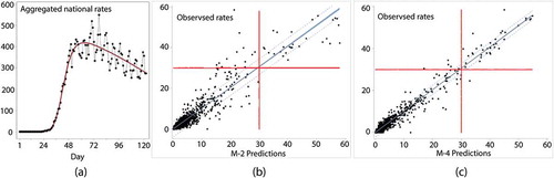
The total the Chinese mainland reported number of cases for the time period is 20,388 (caveat: on 1/21/2020, Yunnan Province had its 1^st and a single new case, whereas on 1/22/2020 it had a new case removed (a negative one); both were set to 0); Figure 3a is a time series graphic portrayal of the increases in number of new cases per 100,000 people during this time horizon plus many days beyond it (an epidemiological curve [i.e. time series plot] for China’s first 95 days). Because the number of cases increases over time with a trajectory initially tracking an S-shaped curve describing exponential growth, and overall tracking a bell-shaped type curve, a logistic transformation of a quadratic function of the number of days since the first case of COVID-19 appeared in the country is a covariate (i.e. the daily average rate is cast as a function of time, and entered in its logarithmic form as a Poisson regression covariate) of the following form:

(7) ${\hat{\mu }}_{\mathrm{d}\mathrm{a}\mathrm{y}}=\frac{11.7127}{1+{\mathrm{e}}^{0.5711-23\left(0.0404\right)-0.0157\left({23}^2\right)}}-\frac{11.7127}{1+{\mathrm{e}}^{0.5711+\left(\mathrm{d}\mathrm{a}\mathrm{y}-23\right)\left(0.0404\right)-0.0157[\left(\mathrm{d}\mathrm{a}\mathrm{y}-23{)}^2\right]}}$(7)

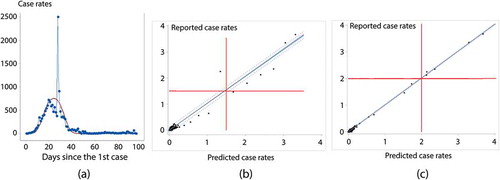
Figure 3. The COVID-19 pandemic in China. Case rates represent the number of cases per 100,000 people. Left (a): an aggregate national time series of rates during the first nearly 100 days, with a superimposed epidemiological curve trend line (solid red line); day 28 (2/12/2020) had a roughly 9-fold increase in Hubei Province (which returned to its previous levels in two days)―because so many people had symptoms with no easy way to test them, authorities appeared to have changed the way COVID-19 was identified. Middle (b): simple space-time RE model (M-2) prediction versus observed case rates for the first 19 days. Right (c): MESTF-RE model (M-4) prediction versus observed case rates for the first 19 days. Dashed lines denote 95% prediction, and shaded area denotes 95% confidence, intervals around a solid trend line

This is the equation describing the superimposed nonlinear trend line in Figure 3a, the country-wide national trend, the curve governments seek to bend. The correspondence between Equation (7)(7) ${\hat{\mu }}_{\mathrm{d}\mathrm{a}\mathrm{y}}=\frac{11.7127}{1+{\mathrm{e}}^{0.5711-23\left(0.0404\right)-0.0157\left({23}^2\right)}}-\frac{11.7127}{1+{\mathrm{e}}^{0.5711+\left(\mathrm{d}\mathrm{a}\mathrm{y}-23\right)\left(0.0404\right)-0.0157[\left(\mathrm{d}\mathrm{a}\mathrm{y}-23{)}^2\right]}}$(7) and the empirical time series scatterplot in Figure 3a yields a linear multiple correlation $R^2$ of 0.47; removing the two extreme outliers (i.e. days 28 and 29) attributable to a definitional change for case reporting increases this $R^2$to 0.89. However, in the context of the space-time diffusion data, in accounts for less than 4% of the spatio-temporal variation (Table 3).

The simple RE zero-inflated Poisson probability model fitting exercise first estimates an RE term together with an intercept and a coefficient for the time covariate number-of-days, given by Equation (7)(7) ${\hat{\mu }}_{\mathrm{d}\mathrm{a}\mathrm{y}}=\frac{11.7127}{1+{\mathrm{e}}^{0.5711-23\left(0.0404\right)-0.0157\left({23}^2\right)}}-\frac{11.7127}{1+{\mathrm{e}}^{0.5711+\left(\mathrm{d}\mathrm{a}\mathrm{y}-23\right)\left(0.0404\right)-0.0157[\left(\mathrm{d}\mathrm{a}\mathrm{y}-23{)}^2\right]}}$(7) , and then decomposes this RE term into a SSRE and a SURE component. Consequently, Figure 3b portrays the scatterplot of predicted versus observed values for the combination of contagion and hierarchical diffusion effects. Figure 3b has the classical V-shaped dispersion of points with increasing rates that characterizes a Poisson random variable: because the mean and variance are the same, deviations from the trend line tend to increase with increasing rates. Matrix $\left(\mathit{I}-{\mathbf{11}}^{\mathrm{T}}/31\right){\mathit{C}}_s\left(\mathit{I}-{\mathbf{11}}^{\mathrm{T}}/31\right)$ has eight, whereas matrix $\left(\mathit{I}-{\mathbf{11}}^{\mathrm{T}}/31\right){\mathit{C}}_H\left(\mathit{I}-{\mathbf{11}}^{\mathrm{T}}/31\right)$ has six, eigenvectors with positive spatial autocorrelation satisfying the condition MC_j/MC₁ ≥ 0.25. Table 2 summarizes results for these two cases, revealing that a hierarchical structure eigenvector is very prominent, and that its contagion spatial structure component, which exhibits strong positive spatial autocorrelation (Figure 4a), plays a prominent role in the RE term. Contagion eigenvectors ${\mathit{E}}_{s,8}$ and ${\mathit{E}}_{s,4}$, and perhaps ${\mathit{E}}_{s,3}$ in part, jointly try to compensate for omitted hierarchical eigenvector ${\mathit{E}}_{H,6}$. Results of zero-inflated Poisson regression appearing in Table 3 confirm that the addition of a hierarchical diffusion element to the analysis merely redistributes statistical explanation and facets between the SSRE and SURE terms without impacting upon their combined outcome represented by their composite RE term alone. The AICc and BIC each decrease by a factor of roughly 16 with the addition of a SSRE plus SURE term, confirming that autocorrelation plays an important role here. Expansion of the SSRE alone to include hierarchical in addition to spatial autocorrelation reduces that terms contribution by a factor of three, indicating the presence of an important hierarchical autocorrelation component.

Figure 4. The contagion-hierarchical diffusion China space-time RE terms; lighter gray denotes relatively small values. Left (a): SSRE (MC = 0.757; $R^2$ = 0.518). Left middle (b): SURE (MC = −0.004). Right middle (c): SSRE_ESTF (MC = 0.640; $R^2$ = 0.607). Right (d): SURE_ESTF (MC = −0.048)

NOTE: eigenvectors are unique to a multiplicative factor of −1, which sometimes results in artificially inverse relationships between maps (e. g. SSRE and SSRE_ESTF). Taiwan is omitted from the model due to data availability.

Table 2. Spatial autocorrelation index and linear regression R² values for selected China RE decompositions

Contagion diffusion only				Contagion plus hierarchical diffusion
		linear regression R^2				linear regression R^2
eigenvector	MCj/MCmax	SSRE	SURE	eigenvector	MCj/MCmax	SSRE	SURE
Es,1	1.0000	0.3093		Es,1	1.0000	0.3093
Es,3	0.7040	0.1398		EH,6	0.4926	0.1543
Es,8	0.2771	0.0946		Es,3	0.7040	0.0540
Es,4	0.6734	0.0630
Cumulative	0.7852	0.6066	0.3934	Cumulative		0.5176	0.4823

NOTE: contiguity MC₁ = 0.930,24; hierarchical MC₁ = 0.992,80.

Table 3. Selected Poisson regression results for the simple China space-time RE specification

feature	${\mu }_{\mathrm{d}\mathrm{a}\mathrm{y}}$ (M-1)	${\mu }_{\mathrm{d}\mathrm{a}\mathrm{y}}$ + SSRE	${\mu }_{\mathrm{d}\mathrm{a}\mathrm{y}}$ + SSRE + SURE (M-2)
spatial autocorrelation only
intercept	−2.716	−3.473	−4.043
deviance	28.61	7.11	2.56
pseudo-R^2	0.038	0.749	0.965
AICc	65,606	12,149	4,135
BIC	65,619	12.166	4,153
$\hat{\pi }$: zero inflation	0.207	0.040	0.020
spatial plus hierarchical autocorrelation
intercept	−2.716	−4.043	−4.043
deviance	28.61	2.56	2.56
pseudo- R^2	0.038	0.965	0.965
AICc	65,606	4,136	4,135
BIC	65,619	4,153	4,153
$\hat{\pi }$: zero inflation	0.207	0.020	0.020

NOTE: the RE = SSRE + SURE arithmetic mean is −1.122, with its Pr(S-W) = 0.002, where S-W denotes the Shapiro-Wilk normality diagnostic statistic; −1.122 − 2.921 = −4.043 The means of SSRE and SURE are 0.

NOTE: AICc denotes the corrected Akaike Information Criterion; BIC denotes the Bayesian Information Criterion.

In addition, Table 3 discloses that this space-time RE specification suffers from a poor RE term estimate, with its mean markedly deviating from zero and its frequency distribution noticeably differing from a bell-shaped normal curve; supplemental model diagnostic outcomes also suggest a lack of conformity to the zero-inflated Poisson specification.

The hierarchical component in the MESTF model specification does more than merely redistribute effects within a limiting composite term like a RE (Table 4, ${\beta }_H$= 0). Rather, it augments contagion diffusion eigenvectors with hierarchical diffusion eigenvectors; although the eigenvectors within each of these sets are orthogonal and uncorrelated, they do not necessarily possess this property across these two sets. Because this spatial analysis involves a complete space-time series, with nT = 589, the number of eigenvectors with MC_j/MC_max ≥ 0.25 is substantially larger than that for the simple space-time RE model (M-2) specification: 136 for the spatial autocorrelation component, of which the stepwise MESTF zero-inflated Poisson regression selected 34, and 127 for the hierarchical autocorrelation component, of which the stepwise regression selected 31 additional vectors (i.e. a total of 65), with these selections being simultaneous. Figure 3c portrays an outcome from these regressions, demonstrating that the MESTF specification shrinks the prediction dispersion vis-à-vis the simple space-time RE (M-2) specification; Table 4 corroborates this contention. These findings imply that inclusion of a hierarchical diffusion component in a spatial diffusion model shows considerable promise for bolstering scientific understanding, prediction, and forecasting of COVID-19 diffusion spread.

Table 4. Selected summary statistics for China model parameter estimation results

Numerical characteristic	RE specification (M-2)	MESTF versions
		ESTF, βH = 0 (M-3)	ESTF (M-3)	ESTF + SSREESTF	ESTF + SSREESTF + SUREESTF (M-4)
Scaling factor	1	1/5	1	1
# eigenvectors	2 contagion + 1 hierarchical	47 contagion	56 contagion + 50 hierarchical	ESTF: 34 contagion + 31 hierarchical; SSREESTF: 4 contagion + 0 hierarchical
Deviance statistic	2.58	5.32	1.54	7.68	1.25
Pseudo-R^2	0.965	0.979	0.997	0.988	0.998
AICc	4,135	5,591	2,647	5,112	2,498
BIC	4,153	5,800	3,804	5,398	2,785
$\hat{\pi }$: zero inflation	0.019	0.050	0.006	0.032	0.008
$\hat{\alpha }$ from Y = α + β$\hat{\mathit{Y}}$	−0.003	−0.010	−0.001	−0.004	−0.000
$\hat{\beta }$ from Y = α + β$\hat{\mathit{Y}}$	1.034	1.112	1.012	1.075	1.009
$\hat{\beta }$day (standard error)	0.7383 (0.0076)	0.7752 (0.0372)	1.1039 (0.0343)	1.0772 (0.0270)	0.9742 (0.0249)

NOTE: AICc denotes the corrected Akaike Information Criterion; BIC denotes the Bayesian Information Criterion.

Figure 5 portrays selected day map patterns of the constructed ESTF, which is a linear combination of eigenvectors selected from the two respective space-time weights matrices. This structural covariate captures a changing role played by the contagion and the hierarchical components, shifting from a hierarchically dominated mixture for the first day ($R^2$ = 0.810, with one contagion and six hierarchical eigenvectors), to a purely hierarchical component for the 14^th day ($R^2$ = 0.429, with three hierarchical eigenvectors), back to a hierarchically dominated mixture for the 19^th day ($R^2$ = 0.862, with two contagions and four hierarchical eigenvectors). This specification outperforms the simple space-time RE model (M-2) specification (Table 4) in rendering a description of the COVID-19 diffusion that already has taken place (i.e. a retrospective description). Including an additional time-invariant RE term essentially does little more than replace a number of the selected eigenvectors (i.e. 44) with a common factor description; this term has both a SSRE and a SURE component, but accounts for less than 3% of the space-time variance through a redistribution from the ESTF term (Table 4), accompanied by noticeable improvements in many of its model diagnostics. Both of the AICc and BIC decreases corroborate this finding.

Figure 5. Selected specimen points-in-time MESTF maps for contagion combined with hierarchy effects for the 31-by-19 China space-time data cube; lighter gray denotes relatively small values. Left (a): day 1 (MC = −0.057). Middle (b): day 14 (MC = 0.143). Right (c): day 19 (MC = 0.117)

Table 4 also reveals that the various specifications yield roughly the same slope coefficient for the global time covariate. In addition, the bivariate regression coefficients, whose theoretical values are 0 for the intercept (α) and 1 for the slope coefficient (β), imply that the MESTF zero-inflated Poisson specification including a hierarchical component renders the closest overall correspondence model results. Of note is that, based upon exploratory simulation experiments, zero inflation appears to induce deviations in the bivariate regression coefficients from their respective theoretical values.

In part, the specifications in this paper parallel the IHME statistical forecasting model (IHME COVID-19 Health Service Utilization Forecasting Team 2020), whose negative critiques emphasize its lack of epidemiological content (for which the RE term substitutes). Nevertheless, the specification in this paper not only incorporates the SIR/SEIR conceptualization (Stehlé et al. 2011), including susceptible (i.e. total population), exposure (i.e. contagion and hierarchical components), and infectious (i.e. new cases) compartments, but also includes a mechanism for mitigation impacts, namely the time-varying national aggregate mean describing the epidemiological curve. Social distancing, for example, can alter this curve, modifying parameter estimates of Equation (7)(7) ${\hat{\mu }}_{\mathrm{d}\mathrm{a}\mathrm{y}}=\frac{11.7127}{1+{\mathrm{e}}^{0.5711-23\left(0.0404\right)-0.0157\left({23}^2\right)}}-\frac{11.7127}{1+{\mathrm{e}}^{0.5711+\left(\mathrm{d}\mathrm{a}\mathrm{y}-23\right)\left(0.0404\right)-0.0157[\left(\mathrm{d}\mathrm{a}\mathrm{y}-23{)}^2\right]}}$(7) in order to describe a flattened version of it.

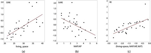
SSRE, SURE, and RE (the sum of SSRE and SURE) model components represent omitted variables. SSRE relates to contagion and hierarchical spatial autocorrelation. As noted previously, construction of this geographic structure builds upon population density, flows in geographic space, and established infrastructure. The amount of living space per person is a prominent covariate of the simple mixed model SSRE term, accounting for more than 40% of its geographic variance (Figure 6a). The ratio of non-agricultural to agricultural population, a type of urban-rural index, accounts for roughly 25% of the simple mixed model SURE term (Figure 6b). In combination, as a RE term, the male-to-female ratio supplements these two covariates, increasing the amalgamated geographic variance accounted for by the linear combination of the three covariates to nearly 50%. The screening of numerous other provincial covariates (e.g. age, health status, population density; e.g. see Likassa 2020) failed to identify other possible omitted variables; this topic merits subsequent future research. Because the two MESTF-RE components account for such a small proportion of space-time variation in the number of new cases, they are left as synthetic variates signifying rather minor omitted variable effects in that specification.

Figure 6. Scatterplots of uncovered covariates of SSRE, SURE, and RE for the simple China space-time RE specification; red denotes a trend line, and solid black dots denote provincial observations. Left (a): SSRE versus living space per person. Middle (b): SURE versus the ratio of non-agricultural to agricultural population (NAP/AP). Right (c): RE versus a linear combination of the preceding two covariates coupled with the ratio of males to females (M/F)

3.2 Diffusion Across the Conterminous US

Paralleling the preceding the Chinese mainland analysis, this section summarizes two principal analytical space-time descriptions of the initial diffusion of COVID-19 across the coterminous US during its first 58 days (i.e. through 4/12/2020) in that country. As before, one is a simple frequentist RE description, whereas the other is a MESTF description, both including a hierarchical diffusion component. The total reported number of new cases for the 58-day time period is 551,563; Figure 7a is an epidemiological curve depicting the increases in number of new cases per 100,000 people during this time horizon plus many days beyond it. Because the number of cases increases over time with a trajectory initially tracking S-shaped exponential growth, immediately followed by a decline in number of cases, a logistic expression coupled with a quadratic function of the number of days since the first case of COVID-19 appeared in the country is a covariate (i.e. the daily average rate is cast as a function of time, and entered in its logarithmic form as a Poisson regression covariate, as for the China analysis) of the following form:

(8) ${\hat{\mu }}_{\mathrm{d}\mathrm{a}\mathrm{y}}=-{\left[\frac{22.18609}{1+{\mathrm{e}}^{6.97888}}\right]}^2+{\left[-0.00037\mathrm{d}\mathrm{a}{\mathrm{y}}^2+\frac{22.18609}{1+{\mathrm{e}}^{6.97888-0.18220\times \mathrm{d}\mathrm{a}\mathrm{y}}}\right]}^2,$(8)

Figure 7. The COVID-19 pandemic in the US. Left (a): an aggregate national time series of rates during the first 122 days, with its nonlinear trend line denoted with red. Middle (b): the simple space-time RE model (M-2) specification predicted versus observed number of cases per 100,000 people for the first 58 days. Right (c): the MESTF-RE model (M-4) specification predicted versus observed number of cases per 100,000 people for the first 58 days. Dashed lines denote 95% prediction, and shaded area denotes 95% confidence, intervals around a solid trend line

which depicts the nonlinear trend line in Figure 7a, the country-wide national trend, the curve US government agencies seek to bend. The correspondence between Equation (8)(8) ${\hat{\mu }}_{\mathrm{d}\mathrm{a}\mathrm{y}}=-{\left[\frac{22.18609}{1+{\mathrm{e}}^{6.97888}}\right]}^2+{\left[-0.00037\mathrm{d}\mathrm{a}{\mathrm{y}}^2+\frac{22.18609}{1+{\mathrm{e}}^{6.97888-0.18220\times \mathrm{d}\mathrm{a}\mathrm{y}}}\right]}^2,$(8) and the empirical time series scatterplot in Figure 7a yields a linear multiple correlation $R^2$ of 0.95 (a bivariate regression describing observed rates with predicted rates yields an intercept term of −0.318, and a slope coefficient of 1.001, nearly identical to their respective theoretical counterpart values of 0 and 1). However, in the context of the space-time diffusion data, in accounts for roughly 26% of the spatio-temporal variation (Table 6).

Table 5 tabulates results for the pure contagion and contagion-hierarchical cases, again revealing that a hierarchical structure eigenvector is most prominent, and that contagion spatial structure displaying strong positive spatial autocorrelation (Figure 8a) plays a very important role, in the US COVID-19 diffusion RE term. The global contagion eigenvector ${\mathit{E}}_{s,2}$ coupled with the regional contagion eigenvector ${\mathit{E}}_{s,4}$ jointly try to compensate for the omitted dominant hierarchical eigenvector ${\mathit{E}}_{H,2}$. Results of the zero-inflated Poisson regression model appearing in Table 6 once more confirm that the addition of a hierarchical diffusion element to the analysis merely redistributes statistical explanation and facets between the SSRE and SURE terms without impacting upon their combined outcome represented by the composite RE term alone.

Figure 8. The contagion-hierarchical diffusion simple US space-time RE terms; lighter gray denotes relatively small values. Left (a): SSRE (MC = 0.697; R² = 0.676). Left middle (b): SURE (MC = −0.189). Right middle (c): SSRE_ESTF (MC = 0.305; R² = 0.176). Right (d): SURE_ESTF (MC = −0.174)

Table 5. Spatial autocorrelation index and linear regression R² values for selected simple US RE decompositions

Contagion diffusion only				Contagion plus hierarchical diffusion
eigenvector	MCj/MCmax	linear regression R^2		eigenvector	MCj/MCmax	linear regression R^2
		SSRE	SURE			SSRE	SURE
Es,2	0.9483	0.2129		EH,2	0.7536	0.2176
Es,4	0.7040	0.1396		Es,13	0.2597	0.1328
Es,13	0.2597	0.1175		Es,2	0.9483	0.1045
Es,10	0.4139	0.0771		Es,1	1.0000	0.0823
Es,1	1.0000	0.0756		Es,10	0.4139	0.0653
				Es,4	0.7040	0.0463
				Es,11	0.3140	0.0275
Cumulative	0.7037	0.6227	0.3773	Cumulative		0.6763	0.3237

NOTE: contiguity MC₁ = 1.016,14; hierarchical MC₁ = 1.519,00.

Table 6. Selected Poisson regression results for the simple US space-time RE specification

feature	${\mu }_{\mathrm{d}\mathrm{a}\mathrm{y}}$	${\mu }_{\mathrm{d}\mathrm{a}\mathrm{y}}$ + SSRE	${\mu }_{day}$ + SSRE + SURE (M-2)
spatial autocorrelation only
intercept	−3.415	−3.925	−4.086
deviance	17.77	13.23	8.58
pseudo-R^2	0.263	0.726	0.896
AICc	744,754	170,247	70,000
BIC	744,772	170,271	70,030
$\hat{\pi }$: zero inflation	0.044	0.028	0.022
spatial plus hierarchical autocorrelation
intercept	−3.415	−3.939	−4.086
deviance	17.77	14.00	8.58
pseudo- R^2	0.263	0.723	0.896
AICc	744,754	165,393	70,000
BIC	744,772	165,417	70,030
$\hat{\pi }$: zero inflation	0.044	0.027	0.022

NOTE: the RE arithmetic mean is −2.383, with its Pr(K-S) = 0.001, where K-S denotes the Kolmogorov-Smirnov statistic (normality diagnostic here); −2.383 − 1.703 = −4.086. The SSRE and SURE means are 0.

NOTE: AICc denotes the corrected Akaike Information Criterion; BIC denotes the Bayesian Information Criterion.

As noted previously, the hierarchical component in the MESTF model not only redistribute effects within a limiting composite term (Table 7, ${\beta }_H$ = 0), but also augments contagion diffusion eigenvectors with hierarchical diffusion eigenvectors. With nT = 2,842, the number of eigenvectors meeting the initial criteria MC_j/MC_max ≥ 0.25 is 652 for the contagion autocorrelation component, with 84 contiguity eigenvectors selected by stepwise regression as being important, and 674 for the hierarchical autocorrelation component, with 87 hierarchical eigenvectors identified as being important, resulting in a total of 171 eigenvectors. Both Poisson regressions require quasi-likelihood estimation (Table 7 reports the scaling factors). Figure 7c shows that the MESTF model that includes both a hierarchical component and a RE term once again shrinks the prediction dispersion as compared to the simple RE (M-2) specification. The SSRE component contains only two hierarchical eigenvectors that account for a trivial amount of space-time variation in the number of new cases (as expected, given that the ESTF should account for all contagion and hierarchical spatial autocorrelation); the RE represents little spatial structure (Figure 8c; it accounts for a mere 18% of the RE variation, which is quite small), and accounts for only a trace amount of space-time variation (Table 7). Coupled with the dramatic AICc and BIC decreases, these findings imply, as their counterparts do for China, that inclusion of a hierarchical diffusion component improves model diagnostics, inferences, and predictions; hierarchical autocorrelation matters.

Table 7. Selected parameter estimation summary statistics for the US models

Numerical characteristic	RE specification (M-2)	MESTF versions
		ESTF, βH = 0 (M-3)	ESTF (M-3)	ESTF + SSREESTF	ESTF + SSREESTF + SUREESTF (M-4)
Scaling factor	1	1/18	1/20	1/5
# eigenvectors	6 contagion + 1 hierarchical	145 contagion	95 contagion + 93 hierarchical	ESTF: 119 contagion + 127 hierarchical; SSREESTF: 2 contagion + 2 hierarchical
Deviance statistic	8.57	32.20	13.82	28.35	5.82
Pseudo-R^2	0.896	0.860	0.961	0.940	0.975
AICc	70,000	72,689	32,270	49,198	25,241
BIC	70,030	73,553	33,380	50,638	26,687
$\hat{\pi }$: zero inflation	0.022	0.025	0.024	0.017	0.015
$\hat{\alpha }$ from Y = α + β$\hat{\mathit{Y}}$	−0.002	−0.047	−0.018	−0.075	−0.015
$\hat{\beta }$ from Y = α + β$\hat{\mathit{Y}}$	1.019	0.977	1.026	1.032	1.017
$\hat{\beta }$day (standard error)	0.9617 (0.0021)	1.0458 (0.0225)	1.0604 (0.0039)	1.0801 (0.0049)	0.9859 (0.0051)

NOTE: AICc denotes the corrected Akaike Information Criterion; BIC denotes the Bayesian Information Criterion.

As Table 7 shows that the slopes for the global time covariate, $\hat{\beta }$_day, are roughly the same across different models, which is a similar finding to that for China. Furthermore, the bivariate regression coefficients, $\hat{\beta }$, once again indicate that the MESTF specification renders the best model fit. As noted previously, zero inflation appears to induce deviations in the bivariate regression coefficients from their respective theoretical values.

Figure 9 portrays selected day map patterns of the ESTF. As the virus diffusion progressed, the roles played by the contagion and the hierarchical components changed, shifting from a mixture of contagion and hierarchical pathways for the first day ($R^2$ = 0.973, with two contagion and five hierarchical eigenvector), to pure hierarchical structure for the 29^th day ($R^2$ = 0.359, with four hierarchical eigenvectors), to a mixture of dominant spatial and hierarchical structure for the 58^th day ($R^2$ = 0.841, with four spatial and two hierarchical eigenvector). Although this specification only slightly outperforms the simple space-time RE specification (Table 7), with the inclusion of an additional time-invariant RE term composed of a very weak SSRE and a stronger SURE component barely enhancing model fit, by accounting for less than 3% of the space-time variance, the almost identical results for both the China and US case studies allow a more refined understanding about the role of hierarchical structure in the diffusion of COVID-19 across a geographic landscape.

Figure 9. Selected specimen points-in-time MESTF maps for contagion combined with hierarchy effects for the 49-by-58 US space-time data cube; lighter gray denotes relatively small values. Left (a): day 1 (MC = 0.487). Middle (b): day 29 (MC = 0.100). Right (c): day 58 (MC = 0.747)

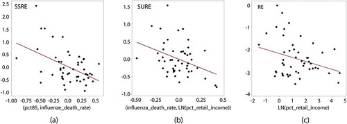
Finally, because the SSRE and SURE model components represent omitted variables, exploration of potential epidemiological factors using the simple space-time RE specification reveal some of the possible missing covariates. The 2018 percentage of population at least 85-years-of-age coupled with the 2019 number of deaths from influenza per 100,000 people correlate with the SSRE term, which relates to contagion and hierarchical autocorrelation, accounting about a fifth of its geographic variance (Figure 10a). The 2019 number of deaths from influenza per 100,000 people coupled with the logarithm of the percentage of 2019 national income generated by the retail sector of the US economy, a type of ubiquitous urban population-at-risk exposure and size index, accounts for more than 10% of the simple mixed model SURE term (Figure 10b). Interestingly, only the logarithm of the percentage of 2019 national income generated by the retail sector of the US economy correlates with their linear combination, the RE term, suggesting that the other covariates are either masked in its aggregate or superfluous; again, future research needs to address this interpretation and meaning of RE terms issue. The screening of numerous other state-level covariates (e.g. temperature, number of days from the appearance of the first US case to a shelter-in-place order, percentage urban population) failed to identify other possible omitted variables. As is the case for the China analysis, because the two MESTF-RE components account for such a small proportion of space-time variation in the number of new cases, they are left as synthetic variates signifying rather minor omitted variable effects in that specification.

Figure 10. Scatterplots of covariates of SSRE, SURE, and RE for the simple US space-time RE specification; red denotes a trend line, and solid black dots denote provincial observations. Left (a): SSRE versus a linear combination of the percentage of 2018 population at least 85 years old plus the 2019 rate of influenza deaths. Middle (b): SURE versus a linear combination of the 2019 rate of influenza deaths plus the 2019 national percentage of retail income. Right (c): RE versus the 2019 national percentage of retail income

3.3 A Comparative Summary

An important objective for conducting scientific research is replicability: when addressing a particular scientific question, a need exists to find consistent empirical results traversing different case studies, each of which has its own dataset. This situation transcends generalizability of findings, and is reminiscent of the age-old geography question about whether or not locations are unique, a question whose contemporary answer entails mutually shared attributes and relationships across locations as well as sense-of-place type attributes and relationships somewhat exclusive to each location. Each of the two preceding COVID-19 spread analyses, one for China and one for the US, offers evidence concerning replicability of the other COVID-19 spread investigation summarized in this paper. This section provides a comparison of these two case studies.

The two preceding nationwide analyses share various commonalities. The national trend lines for both China and the US (Figures 3a and 7a) are quadratic in nature, and confirm that both a contagion and a hierarchical diffusion pathway operate in each country without acknowledging where new cases occur, and without compensating for them as omitted variables when model M-1 is extended to models M-2 and M-4; the hierarchical element is unmistakable, and should not be ignored in models of disease spread (most publications cited in the literature review of this paper overlook it). The most suitable probability model description for both countries is a zero-inflated Poisson specification that accounts for the presence of positive spatial and temporal autocorrelation, with a rather stable estimate of roughly 1%-2% excess zeroes; however, this percentage of zeroes is so small that a zero-inflated specification may not be warranted. The MESTF (M-4) specification outperforms the simple space-time RE (M-2) specification based upon a suite of distinct metrics, in part because the constructed ESTF relaxes the inflexibility of the time-invariant space-time RE term by capturing spatial autocorrelation fluctuations over time. Nevertheless, the SSRE-SURE decomposition of the simple RE term reflects approximately the same degree of positive spatial autocorrelation (as indexed by the MC) for both countries. Clues furnished by each of these components allowed successful identification of substantive epidemiological-relevant covariates to statistically explain a portion of them for both countries; these covariates constitute potential omitted variables. Furthermore, an additional RE term for the MESTF specification is trivial but significant for each country, with its inclusion improving a number of diagnostics (e.g. the deviance statistic). Finally, the MESTF-RE (M-4) hybrid specification accounts for approximately 95% or more of the space-time variation in new case rates both for China and for the US.

A comparison of the two preceding analyses also uncovers an assortment of differentiators. Foremost is the number of days required for the spread of COVID-19 to all provinces/states in each country (e.g. 14 days for China, and 33 days for the US), somewhat of a surprise given that the two territories are roughly equal in area extent; similarly, the aggregate number of reported new cases (by the 19^th day, China had 20,388, whereas the US had 111, recorded; by the 58^th day, these recorded numbers respectively were 80,763 and 551,563). The functional form (which would have the same identified specification as that for the US case if the initial China time series comprised considerably more than 19 days) as well as the role of the national trend line vary between these two countries: China’s epidemiological curve [Equation (7)(7) ${\hat{\mu }}_{\mathrm{d}\mathrm{a}\mathrm{y}}=\frac{11.7127}{1+{\mathrm{e}}^{0.5711-23\left(0.0404\right)-0.0157\left({23}^2\right)}}-\frac{11.7127}{1+{\mathrm{e}}^{0.5711+\left(\mathrm{d}\mathrm{a}\mathrm{y}-23\right)\left(0.0404\right)-0.0157[\left(\mathrm{d}\mathrm{a}\mathrm{y}-23{)}^2\right]}}$(7) , Figure 3a] is only exponential in form, whereas the one for the US [Equation (8)(8) ${\hat{\mu }}_{\mathrm{d}\mathrm{a}\mathrm{y}}=-{\left[\frac{22.18609}{1+{\mathrm{e}}^{6.97888}}\right]}^2+{\left[-0.00037\mathrm{d}\mathrm{a}{\mathrm{y}}^2+\frac{22.18609}{1+{\mathrm{e}}^{6.97888-0.18220\times \mathrm{d}\mathrm{a}\mathrm{y}}}\right]}^2,$(8) , Figure 7a] has an additional non-exponential quadratic term; and, the percent of space-time variance accounted for by the China trend line (model M-1) is scarcely 4% (Table 3), whereas it exceeds 25% (Table 6) for the US. The simple space-time RE model (M-2) specification decompositions yield essentially a 50 - 50 split for China, but roughly a 2/3-1/3 split for the US (see the values of SSRE and RE for the contagion plus hierarchical diffusion model, Tables 2 and 5). The 15.8% of space-time eigenvectors required to construct an ESTF for the US is conspicuously less than the 41.4% required for the China analysis, although weighting by the difference in numbers of areal-unit-days increases it to a conspicuously larger 76.1%. Although the sets of identified SURE-SSRE covariates for the simple space-time RE (M-2) specification reflect potentially omitted epidemiological factors, they notably differ for the two countries: China has living space per person for its SSRE component, the ratio of non-agricultural to agricultural population for its SURE component, and the addition of the ratio of males to females for its aggregate RE term; the US has percentage of 2018 population at least 85 years old plus the 2019 rate of influenza deaths for its SSRE component, the 2019 rate of influenza deaths plus the 2019 national percentage of retail income for its SURE component, and only the 2019 national percentage of retail income for its aggregate RE term. Finally, after accounting for approximately 97% of the space-time variance in new cases, the remaining overdispersion (i.e. extra-Poisson variation) for the US M-4 model is more than seven times that for the China M-4 model.

In summary, evidence exists supporting the replication of primary findings about the spatial diffusion of COVID-19 across a national geographic landscape, one that also is nuanced and partially idiosyncratic in terms of individual locations.

4. Short-Term Forecasting

The preceding results describe new cases for the initial disease waves across two countries. However, the existence of disease diffusion motivates ongoing compilations―released daily tabulations of new cases for many subsequent days immediately following those used to complete these preceding spatial analyses—which furnish a predictive testbed type of environment for the two spatial statistical model specifications. Because the respective time horizons cover the periods during which COVID-19 spread across the Chinese mainland and the coterminous US, forecasts based upon them entail only in situ expansion of the virus in each country’s population. Griffith and Chun (2014), and Griffith and Paelinck (2009), furnish the methodological foundation for this section; their approaches aim to protect against outlier forecasts (Cheng and Yang 2015). The tactic involves forecasting the total national number of new cases with a first-order autoregressive time series model. Next, each of these forecasted sums is divided by the sum of its corresponding forecasted spatial series total, with each of the forecasted spatial series then multiplied by its respective resulting weight (Table 8); this computational adjustment ensures that the total forecasted number of, here, predicted new cases is consistent with the total number of observed new cases. Meanwhile, Tan and Chen (2020) posit an important perspective characterizing this section of this paper: forecasting the geographic spread of a disease governed by contagious and hierarchical pathways is analogous to weather forecasting in that only short-term forecasts tend to be reasonably accurate because a plethora of space-time varying interacting factors coupled with socio-economic/demographic and behavioral uncertainties operate in a dynamic geographic landscape. Accordingly, this section presents only about a week of forecasts.

Table 8. Bivariate linear regression coefficients and R² values for additional eight days of new cases forecasted by the two space-time models for China

day	weight	Complete data			Data without Hubei Province
		$\hat{\alpha }$	$\hat{\beta }$	R2	$\hat{\alpha }$	$\hat{\beta }$	R2
space-time RE model (M-2) specification
20	1.00718	−0.067	1.515	0.997	0.003	0.649	0.763
21	0.96099	−0.063	1.449	0.996	0.007	0.561	0.720
22	0.92702	−0.042	1.198	0.997	0.006	0.576	0.617
23	0.90307	−0.072	1.411	0.996	0.002	0.448	0.596
24	0.88760	−0.043	1.031	0.995	0.015	0.276	0.447
25	0.87955	−0.066	1.328	0.995	0.009	0.329	0.504
26	0.87942	−0.052	1.074	0.995	0.010	0.257	0.406
27	0.88686	−0.033	0.847	0.994	0.012	0.247	0.300
All		−0.056	1.241	0.965	0.007	0.430	0.509
MESTF-RE model (M-4) specification
20	0.88258	−0.070	1.570	0.992
21	1.14938	−0.167	1.887	0.835
22	0.28942	0.096	0.426	0.049
23	0.00741	0.205	−0.043	0.002
24	0.00032	0.157	−0.030	0.002
25	0.00005	0.193	−0.064	0.003
26	0.00007	0.155	−0.056	0.003
27	0.01457	0.133	−0.070	0.005
All		0.130	0.256	0.048

Models M-2 and M-4 generate the best forecasts, and hence are the focus of this section. The most advantageous traits of the M-2 model are its simplicity and parsimony. The single most advantageous benefit of the M-4 model is its best overall diagnostics, particularly efficiency attributable to a better accounting of variability and a better linear alignment between fitted and observed values.

4.1 China Mainland Provincial Level Forecasts

Producing eight days of forecasts avoids the two anomalous days in the China mainland dataset. Hubei Province (which houses Wuhan, the epicenter of COVID-19) is a blatant outlier (see Figure 11) in this forecasting exercise. In order to exemplify its impact upon forecast assessment, Table 8 reports forecasting results with and without Hubei province. Not surprisingly, forecast goodness-of-fit results improve when the dataset contains Hubei Province. Figures 11a and 11c highlight this situation, resembling the fitting of a straight line to only two points.

Figure 11. Scatterplots with trend lines for the eight days of forecasts for China; each color denotes a different day. Left (a): all data; simple RE model. Left middle (b): Hubei Province removed; simple RE model. Right middle (c): all data; MESTF-RE model. Right (d): the overall best day forecast (#20) – the dashed lines denote 95% prediction, and the shaded area denotes 95% confidence, intervals around the solid trend line; MESTF-RE model

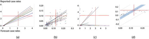
Figure 11b as well as the bivariate regression results appearing in Table 8 imply that the simple space-time RE model (M-2) specification renders sounder forecasts than the MESTF-RE (M-4) specification (e.g. its bivariate regression slope coefficients are closer to one); Figure 11d suggests that a one-step MESTF-RE forecast is good, but most of this model’s other forecasts appear to suffer from a lack of inertia buildup [i.e. too few initial time periods, which Hanke and Wichern (2013) argue should be at least 50, rather than merely 19]. The simple space-time RE (M-2) specification scatterplots display good performance regardless of the inclusion of Hubei Province; the MESTF-RE (M-4) specification furnishes an inferior performance, with useless forecasts after two-steps ahead. The simple space-time RE (M-2) specification without Hubei Province also suggests that the rate forecasts deteriorate with the passing of time, an expectation alluded to by forecasts from the MESTF-RE (M-4) specification. Nevertheless, both specifications stress the important diffusion role played by a geographic hierarchy pathway.

4.2 US State Level Forecasts

Producing eight days of US forecasts furnishes a benchmark for evaluating the preceding China COVID-19 diffusion results. The US time horizon is much longer, permitting an accumulation of inertia to occur in its geographic landscape, as is reflected in Table 9 tabulations, which summarize results for this case. Again, the simple space-time RE (M-2) specification outperforms the MESTF-RE (M-4) specification, but not as dramatically as in the China case. These types of differences also may signal mitigation strategy variations beyond the national trend, such as the level of quarantine. Both specifications render respectable forecasts, as is indicated by their $R^2$ values. As with the China analysis, a clear deterioration of forecasts over the time horizon is not apparent.

Table 9. Bivariate linear regression coefficients and R² values for additional eight days of new cases forecasted by the two space-time models for the US

day	space-time RE model (M-2) specification				MESTF-RE model (M-4) specification
	weight	$\hat{\alpha }$	$\hat{\beta }$	R^2	weight	$\hat{\alpha }$	$\hat{\beta }$	R^2
59	0.89475	5.294	0.750	0.643	1.22292	2.624	0.559	0.576
60	0.88254	4.342	0.888	0.787	1.81502	1.530	0.578	0.481
61	0.90881	4.645	0.951	0.797	1.98532	1.616	0.580	0.283
62	0.94501	4.995	0.963	0.791	2.39598	0.083	0.729	0.510
63	0.92727	5.180	0.816	0.708	2.29743	1.161	0.647	0.546
64	0.90666	5.325	0.778	0.666	2.78655	1.475	0.589	0.545
65	0.91004	4.850	0.705	0.665	3.48831	1.912	0.443	0.261
66	0.92536	7.805	0.754	0.475	2.58464	3.468	0.422	0.227
All		1.622	0.827	0.681		1.788	0.564	0.412

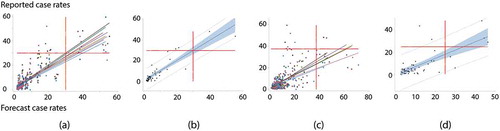
Figure 12 furnishes scatterplots for the sets of forecasts, portraying relatively less dispersion by the forecasted simple RE rates from their actual rate counterparts (Figures 12a and 12c). This smaller dispersion also characterizes the selected best single day results (Figures 12b and 12d).

Figure 12. Scatterplots with trend lines for the eight days of forecasts for the US; each color denotes a different day. Left (a): all data; simple RE model. Left middle (b): the overall best day forecast (#62) – the simple RE model. Right middle (c): all data; MESTF-RE model. Right (d): the overall best day forecast (#62) – the MESTF-RE model. The dashed lines denote 95% prediction, and the shaded area denotes 95% confidence, intervals around the solid trend line

4.3 Forecast Propositions

The preceding analyses imply a number of salient forecast propositions. Foremost is the assertion that

a prevailing geographic hierarchy (e.g., one based upon a national urban system’s spatial structure) delivers an important conduit for channeling the diffusion of COVID-19 across an active geographic landscape.

In other words, based upon data analytic results for both the simple space-time RE (M-2) and the MESTF-RE (M-4) specifications, hierarchical diffusion pathways play an influential channeling role that cannot be ignored. Meanwhile, another appropriate postulate is that

the MESTF-RE (M-4) specification tends to supply a superior retrospective description of the COVID-19 diffusion, whereas the simple space-time RE (M-2) specification tends to supply superior prospective short-term forecasts.

This contention is consistent with the IHME COVID-19 model specification, which is built upon this type of RE foundation. In addition, it echoes the MESTF-RE predictive failure highlighted by Table 7, and somewhat refuted by predictive results reported in Table 8. Furthermore, Tables 7 and 8 imply the following hypothesis:

a direct relationship exists between the length of time series constituting a space-time series and the number of future time intervals for which the MESTF-RE (M-4) specification furnishes reasonable forecasts.

The time series length for China is 19, with two future reasonable forecasts, whereas the time series length for the US is 58, with at least six future reasonable forecasts.

A final prominent assertion is that:

both the simple RE (M-2) and MESTF-RE (M-4) specifications need initial space-time data in order to provide forecasts, currently reducing them to uninformative equations in the first days of the diffusion of a disease such as COVID-19.

Space-time inertia must accumulate in an active geographic landscape before forecasts with the two model specifications become feasible; Hanke and Wichern (2013) argue that at least 50 data collection points in time need to transpire. This feature reveals a simulation experiments gap requiring future research attention: systematic explorations of synthetic populations need to establish practical assumptions and their implied space-time trajectories for consideration at the very beginning of a disease’s diffusion. The subsequent conceptualization needs to incorporate, among other facets, the prevailing spatial hierarchy.

5. Conclusions

A primary finding of the research summarized in this paper is that inclusion of a hierarchical diffusion component matters when predicting spatial diffusion spread, at least of COVID-19; both the China and the US case studies support this contention, which seems intuitive, although apparently disregarded in most contemporary COVID-19 geographic spread literature. This verdict confirms a contention repeatedly found in the spatial diffusion literature.

Both the simple space-time RE (M-2) and MESTF-RE (M-4) specifications furnish useful conceptualizations for short-term forecasting of the magnitude and location of diffusion once a space-time dataset becomes available. In their present, simplest, and rather unsophisticated forms, these two formulations allow short-term (i.e. a few days to about a week) forecasts of COVID-19 diffusion. Each has its advantages and disadvantages. The simple space-time RE (M-2) specification presents fewer computational challenges, gives more respectable forecasts (e.g. moderately good agreement with data, consistently into the future), but merely reallocates latent spatial and hierarchical structure effects from a SURE to a SSRE term. Although this reallocation may be irrelevant to prediction/forecasting, ignoring it distorts understanding of the diffusion process. In contrast, the MESTF-RE (M-4) specification more accurately describes the space-time data used to estimate/calibrate its forecasting equation, enhancing a contagion diffusion description with a supplemental hierarchical diffusion description, displays selected preferable properties (e.g. its bivariate regression slope coefficient is close to one; Tables 4 and 7), but produces forecasts that deteriorate more rapidly over time, with more forecasts outside of its narrower prediction intervals (the general V-shape of these intervals reflects the Poisson random variable nature of the new cases counts). The quality of these forecasts seems on par with the popular next-five-days meteorological weather forecasts offered to the general public. Furthermore, these specific forecasts suggest a strategy of daily updating a disease diffusion model’s estimation in order to produce a continuous sequence of next-five-day forecasts, similar to weather forecast practices. One important implication here is that both formulations could be bolstered by enhancing their respective specifications.

Another salient finding is that a preponderance of zeroes in the first half of a spatial diffusion process—representing locations to which the disease has not yet diffused—may not necessarily support the use of a zero-inflated counts model specification (e.g. Tables 3 and 7 report very small probabilities of an excessive number of zeroes, once a specification accounts for space-time autocorrelation). An important advantage of employing this specification is that it is pertinent during the initial spread of the disease during which many locations have yet to experience the disease, and as the relative number of zeroes diminishes, resulting in their appearing less excessive as more locations become initially contaminated by the disease, the estimate goes to zero (whereas, excluding it from the model specification forces the Poisson probability model to treat all zeroes as a Poisson realization, rather than some as the outcome of not yet being exposed to the disease).

An integration of these myriad conclusions delivers three interesting propositions that hint at a future research agenda. One concerns the lead time necessary for generating space-time forecasts. Another focuses on the specification of the geographic hierarchical structure and the geographic resolution of the areal units. And the third consideration has to do with alternative spatial statistical model specifications.

The China data analysis gives rise to concerns over data quality and the estimation of ${\mu }_{day}$. First, its national aggregate time series, the sequential data used to establish an epidemiological curve for the country, has two extreme outlier days that raise data quality questions. Results for the MESTF-RE forecasts tend to corroborate this questionable data quality contention (Table 8 versus Table 9 contents), although an alternative explanation for this particular anomalous outcome is that the China space-time series is too short to generate more extended forecasts. Second, considering a longer time horizon with the two aberrations smoothed yields the following description of its national mean rate:

(9) $\begin{array}{r}{\hat{\mu }}_{\mathrm{d}\mathrm{a}\mathrm{y}}=-{\left[-0.00117(12{)}^2+\frac{4.07033}{1+{\mathrm{e}}^{5.66503-0.24291(12)}}\right]}^2\\ +{\left[-0.00117(\mathrm{d}\mathrm{a}\mathrm{y}+12{)}^2+\frac{4.07033}{1+{\mathrm{e}}^{5.66503-0.24291(\mathrm{d}\mathrm{a}\mathrm{y}+12)}}\right]}^2\end{array}$(9)

which has a pseudo-R² of 0.94 with removal of the two outliers. In other words, although Equations (7)(7) ${\hat{\mu }}_{\mathrm{d}\mathrm{a}\mathrm{y}}=\frac{11.7127}{1+{\mathrm{e}}^{0.5711-23\left(0.0404\right)-0.0157\left({23}^2\right)}}-\frac{11.7127}{1+{\mathrm{e}}^{0.5711+\left(\mathrm{d}\mathrm{a}\mathrm{y}-23\right)\left(0.0404\right)-0.0157[\left(\mathrm{d}\mathrm{a}\mathrm{y}-23{)}^2\right]}}$(7) and (9(9) $\begin{array}{r}{\hat{\mu }}_{\mathrm{d}\mathrm{a}\mathrm{y}}=-{\left[-0.00117(12{)}^2+\frac{4.07033}{1+{\mathrm{e}}^{5.66503-0.24291(12)}}\right]}^2\\ +{\left[-0.00117(\mathrm{d}\mathrm{a}\mathrm{y}+12{)}^2+\frac{4.07033}{1+{\mathrm{e}}^{5.66503-0.24291(\mathrm{d}\mathrm{a}\mathrm{y}+12)}}\right]}^2\end{array}$(9) ) for China contain a time shift, Equations (8)(8) ${\hat{\mu }}_{\mathrm{d}\mathrm{a}\mathrm{y}}=-{\left[\frac{22.18609}{1+{\mathrm{e}}^{6.97888}}\right]}^2+{\left[-0.00037\mathrm{d}\mathrm{a}{\mathrm{y}}^2+\frac{22.18609}{1+{\mathrm{e}}^{6.97888-0.18220\times \mathrm{d}\mathrm{a}\mathrm{y}}}\right]}^2,$(8) and (9(9) $\begin{array}{r}{\hat{\mu }}_{\mathrm{d}\mathrm{a}\mathrm{y}}=-{\left[-0.00117(12{)}^2+\frac{4.07033}{1+{\mathrm{e}}^{5.66503-0.24291(12)}}\right]}^2\\ +{\left[-0.00117(\mathrm{d}\mathrm{a}\mathrm{y}+12{)}^2+\frac{4.07033}{1+{\mathrm{e}}^{5.66503-0.24291(\mathrm{d}\mathrm{a}\mathrm{y}+12)}}\right]}^2\end{array}$(9) ) argue for the existence of a common national number of new cases time series description.

The spatial weights matrices that capture the spatial autocorrelation information are at the core of the MESTF models. Specification of the hierarchical structure and adoption of a specific areal partitioning directly affect the resulting spatial weights matrices. As we indicate in the methodology section, the hierarchical structures used in this paper were constructed based upon literature research coupled with necessarily being parsimonious. More realistic and sophisticated specifications of the hierarchical structures for both countries would surely further our understanding on the effects of hierarchical diffusion. For contagion diffusion, the effects of the geographic units, or spatial resolution, are another factor to be explored further. Both China and the US would profit from application of the two forecasting models at the county level. Doing so would enable an explicit integration of the respective national urban hierarchies into their hierarchical diffusion components. A fundamental drawback of this effort is that the space-time dataset dimensions would be approximately 2,851-by-19 for the China case, and 3,111-by-58 for the US case, requiring enormous structure matrices (whose dimensions are the square of this number) demanding numerically intensive computing; as the preceding space-time weights matrices indicate, part of the accompanying computational burden could be alleviated by exploiting the Kronecker product operator: individual matrix eigenfunctions, which are much smaller in size, can be combined with Kronecker products to produce the required extremely large space-time matrices.

With regard to spatial statistical model specifications, a spatial panel model is an alternative to the GLMM approach employed in this paper (e.g. Elhorst 2014), a viewpoint that warrants some commentary. Mechanically, they are very similar techniques. Both deal with doubly subscripted terms, with one usually being time for panel data; the mixed model conceptualizations in this paper also have a time subscript. Their most important difference is their treatment of substantive covariates—in this paper, solely the national trend term—which when included in the GLMM corresponds to the panel data time component. The mixed model conceptualization posits a two-level regression: the first level is an individual regression for each areal unit, with the second level regression statistically explaining variation in the first-level regression coefficients. The panel data random effects model is equivalent to this formulation; these models diverge for the panel data fixed effects specification. Meanwhile, in order to maintain comparability with a space-time autoregressive formulation (Cliff et al. 1975), the analysis summarized in this paper employed a mixed model conceptualization. If evidence supports a fixed effects specification—the preceding fixed and random effects comparisons initialize this evaluation—future research should extend this study using a spatial panel analysis.

Besides the spatial panel approach, the introductory literature review highlights that existing relevant mainstream COVID-19 spatial analyses utilize mixed model specifications, Bayesian analysis, and space-time conceptualizations. Findings summarized in this paper differ from those for these earlier publications, in part because our specification more closely resembles a spatial panel analysis design coupled with employing MESF and MESTF methodology in a fixed/random effects style. In doing so, we explicitly uncover a geographic hierarchical component to better understand the disease’s diffusion, and to demonstrably exploit RE terms to identify potential omitted variables. Our approach also intentionally addresses excess zeroes.

Another valuable prospective to undertake would be to express the geographic spread in probabilistic terms, where probabilities are based upon both a contagion and a hierarchical configuration of geographic space, and forecast the potential of leaps and creeps of a disease across an active geographic landscape. Moreover, once the initial COVID-19 case appeared in Wuhan or WA, respectively identifying the most probable sequence of its spread to the rest of Chinese mainland and the coterminous US, once more with a day-by-day conditional forecast of its next appearance locations (e.g. province or state), would have been tremendously beneficial for effectively reacting to the present pandemic.

Finally, the notion of Spatial Stratified Heterogeneity (SSH; i.e. geographic variance within more than between strata) may be germane to this type of analysis (Wang, Zhang, and Fu 2016), although to date it does not seem to have been applied to the geographic diffusion of diseases in any meaningful way. This is a potential future research topic, too.

In conclusion, the diffusion of COVID-19 across Chinese mainland as well as the coterminous US followed both contagion and hierarchical geographic pathways. A simple space-time RE (M-2) specification furnishes the best description of the space-time unfolding of this diffusion process, one that supports short-term forecasts. Many common realized features appear in the diffusion of COVID-19 across both national geographic landscapes, confirming the reasonableness of its IHME model description for the US, and suggesting the need to establish such a model for China. In addition, as the exploratory analyses of the RE terms reveals, this model formulation should be accompanied by a search for epidemiologically relevant covariates that describe the sets of SSRE and SURE terms.

Acknowledgments

The authors would like to thank the constructive comments from the anonymous reviewers.

Data Availability Statement

The data that support the findings of this study are available in the public domain:

1. Daily counts of COVID-19 cases by provinces, China, are available from the Harvard Dataverse at https://doi.org/10.7910/DVN/MR5IJN.

2. The 2010 China Population data set is available from the National Bureau of Statistics of China at http://www.stats.gov.cn/english/Statisticaldata/CensusData.

3. Daily counts of COVID-19 cases by states, USA, are compiled by the Johns Hopkins University Center for Systems Science and Engineering (CSSE) and available at https://github.com/CSSEGISandData/COVID-19.

4. The 2019 Annual State Population Estimates for the US is available at the US Census Bureau Web site https://www.census.gov/data/tables/time-series/demo/popest/2010s-state-total.html.

5. Spatial weights matrices for China were derived from the provincial boundary data set available from the Harvard Dataverse at https://doi.org/10.7910/DVN/DBJ3BX.

6. Spatial weights matrices for the US were derived from the US Census Bureau at https://www.census.gov/geographies/mapping-files/time-series/geo/carto-boundary-file.html.

Additional information

Notes on contributors

Daniel Griffith

Bin Li is a professor of Geography at Central Michigan University, United States. He received a B.S. from South China Normal University, M.S. from University of Nebraska, and Ph.D. in Geography from Syracuse University. He conducts research and teaches courses in GIS, cartography, spatial statistics, and economic geography.

Bin Li

Daniel A. Griffith is an Ashbel Smith professor of Geography and Geospatial Information Sciences, School of Economic, Political and Policy Sciences, at the U. of Texas at Dallas. He earned an undergraduate degree in mathematics, and graduate degrees in statistics and geography, receiving his PhD from the University of Toronto in 1978. He held previous faculty positions at the U. of Miami, Syracuse U. (SU), SUNY/Buffalo, and Ryerson U. in Toronto. His many past service roles include Chair of the SU Geography Department and the International Spatial Accuracy Research Association (ISARA) Steering Committee, and editor of Geographical Analysis. His over 200 publications about spatial accuracy, spatial statistics, urban and regional economics, and spatial epidemiology appear in geography, computer science, economics, epidemiology, regional science, statistics, and mathematics journals. He has been recognized by the ISARA (Founders Award, Peter Burrough medal), the American Association of Geographers (J. Warren Nystrom dissertation award, distinguished research honors, elected Fellow), the Fulbright Program (Research Fellowship, Senior Specialist), the American Statistical Association (USDA-NASS Research Fellowship, elected Fellow), the John Simon Guggenheim Memorial Foundation, the Leverhulme Trust, and the University Consortium of Geographic Information Science (UCGIS; Research Award, elected Fellow). He also has been elected a Regional Science Association International, an American Association for the Advancement of Science (AAAS), and a Spatial Econometrics Association fellow, and in 2017 he was elected a foreign fellow of the Royal Society of Canada.

Notes

1. See https://www.peakbagger.com/pbgeog/histmetropop.aspx

2. https://www.census.gov/data/tables/time-series/demo/popest/2010s-total-metro-and-micro-statistical-areas.html

3. https://metrocosm.com/traffic-flow-maps/

4. https://www.nasa.gov/offices/oct/home/tech_life_facet.html

5. https://www.earthlymission.com/wp-content/uploads/2015/07/where-we-live-usa.jpg

6. https://dataverse.harvard.edu/dataset.xhtml?persistentId = doi:10.7910/DVN/MR5IJN

7. https://github.com/CSSEGISandData/COVID-19

8. http://www.stats.gov.cn/english/Statisticaldata/CensusData/or http://www.stats.gov.cn/tjsj/pcsj/rkpc/6rp/indexce.htm

9. https://www.census.gov/data/tables/time-series/demo/popest/2010s-state-total.html

10. https://coronavirus.jhu.edu/us-map

References

- Borchert, J. 1967. American metropolitan evolution. Geographical Review 57: 301–332.
- Borchert, J. 1972. America’s changing metropolitan regions. Annals of the Association of American Geographers 62: 352–373.
- Briz-Redón, Á., and Á. Serrano-Aroca. 2020. “A Spatio-temporal Analysis for Exploring the Effect of Temperature on COVID-19 Early Evolution in Spain.” Science of the Total Environment 728: 138811. doi:https://doi.org/10.1016/j.scitotenv.2020.138811.
- Cheng, G., and Y. Yang. 2015. “Forecast Combination with Outlier Protection.” International Journal of Forecasting 31 (2): 223–237. doi:https://doi.org/10.1016/j.ijforecast.2014.06.004.
- Christaller, W. 1966. Central places in southern Germany. Vol. 10. Prentice-Hall.
- Cliff, A., P. Haggett, J. Ord, and G. Versey. 1981. Spatial Diffusion: An Historical Geography of Epidemics in an Island Community. NY: Cambridge U. Press.
- Cliff, A., P. Haggett, J. Ord, K. Bassett, and R. Davies. 1975. Elements of Spatial Structure: A Quantitative Approach. London: Cambridge U. Press.
- Danon, L., E. Brooks-Pollock, M. Bailey, and M. Keeling. 2020. “A Spatial Model of CoVID-19 Transmission in England and Wales: Early Spread and Peak Timing.” medRxiv. doi:https://doi.org/10.1101/2020.02.12.20022566.
- de Jong, P., C. Sprenger, and F. Van Veen. 1984. “On Extreme Values of Moran’s I and Geary’s c.” Geographical Analysis 16 (1): 17–24.
- Dobis, E., M. Delgadoa, R. Florax, and P. Mulderb. 2015. “The Significance of Urban Hierarchy in Explaining Population Dynamics in the United States.” Paper presented at the 2015 Agricultural and Applied Economics Association (AAEA) & Western Agricultural Economics Association (WAEA) Joint Annual Meeting, July 26-28, San Francisco, CA. http://ageconsearch.umn.edu/record/205869/files/Dobis_et_al_AAEA2015.pdf
- Elhorst, J. 2014. “Spatial Panel Data Models.” InChap 3, Spatial Econometrics, edited by Elhorst, J., 37–93. Berlin: Springer.
- Fanelli, D., and F. Piazza. 2020. “Analysis and Forecast of COVID-19 Spreading in China, Italy and France.” Chaos, Solitons and Fractals, Online in ScienceDirect 134: 109761. doi:https://doi.org/10.1016/j.chaos.2020.109761.
- Frondel, M., and C. Vance. 2010. “Fixed, Random, or Something in Between? A Variant of HAUSMAN’s Specification Test for Panel Data Estimators.” Economic Letters 107 (3): 327–329. doi:https://doi.org/10.1016/j.econlet.2010.02.007.
- Giuliani, D., M. Dickson, G. Espa, and F. Santi. 2020.“Modelling and Predicting the Spread of Coronavirus (COVID-19) Infection in NUTS-3 Italian Regions.” arXiv Preprint. arXiv: 2003.06664.
- Gould, P. 1969. Spatial Diffusion. Resource Paper No. 4. Washington, D.C.: Association of American Geographers, Commission on College Geography.
- Griffith, D. 2005. “A Comparison of Four Analytical Disease Mapping Techniques as Applied to West Nile Virus in the Coterminous United States.” International Journal of Health Geographics 4 (1): 1–14. doi:https://doi.org/10.1186/1476-072X-4-18.
- Griffith, D. 2012. “Space, Time, and Space-time Eigenvector Filter Specifications that Account for Autocorrelation.” Estadística Española 54 (177): 7–34.
- Griffith, D., and J. Paelinck. 2009. “Specifying a Joint Space- and Time-lag Using a Bivariate Poisson Distribution.” Journal of Geographical Systems 11 (1): 23–36. doi:https://doi.org/10.1007/s10109-008-0075-3.
- Griffith, D., and Y. Chun. 2014. “An eigenvector spatial filtering contribution to short range regional population forecasting.” Economics and Business Letters 3 (4): 208–217. doi:https://doi.org/10.17811/ebl.3.4.2014.208-217.
- Griffith, D., Y. Chun, and B. Li. 2019. Spatial Regression Analysis Using Eigenvector Spatial Filtering. Cambridge, MA: Elsevier.
- Griffith, D. A. 1996. “Spatial autocorrelation and eigenfunctions of the geographic weights matrix accompanying geo‐referenced data.” Canadian Geographer/Le Géographe canadien 40(4): 351–367.
- Griffith, D. A. 2002. “A spatial filtering specification for the auto-Poisson model.“ Statistics & probability letters 58(3): 245–251.
- Griffith, D. A. 2004. “A spatial filtering specification for the autologistic model.“ Environment and Planning A 36(10): 1791–1811.
- Gu, C-l., and H-f. Pang. 2008. “Study on Spatial Relations of Chinese Urban System: Gravity Model Approach (In Chinese).” Geographical Research 27 (1): 1–12.
- Guliyev, H. 2020. “Determining the Spatial Effects of COVID-19 Using the Spatial Panel Data Model.” Spatial Statistics, Online in ScienceDirect 38: 100443. doi:https://doi.org/10.1016/j.spasta.2020.100443.
- Hägerstrand, T. 1953. Innovation Diffusion as a Spatial Process [Innovationsförloppet Ur Korologisk Synpunkt]. postscript and translation by A. Pred (1967) with the assistance of G. Haag. Chicago:University of Chicago Press.
- Han, R., H. Cao, and Z. Liu. 2018. “Studying the Urban Hierarchical Pattern and Spatial Structure of China Using a Synthesized Gravity Model.” Science China: Earth Sciences 61 (12): 1818–1831. doi:https://doi.org/10.1007/s11430-016-9191-5.
- Hanke, J., and D. Wichern. 2013. Business Forecasting. 9th ed. Upper Saddle River, NJ: Pearson.
- Hansen, N. 1975. A critique of economic regionalizations of the United States. IIASA Research Report RR-75-032. Laxenburg, Austria: International Institute of Applied Systems Analysis.
- IHME COVID-19 Health Service Utilization Forecasting Team. 2020. “Forecasting the Impact of the First Wave of the COVID-19 Pandemic on Hospital Demand and Deaths for the USA and European Economic Area Countries.” medRχiv. doi:https://doi.org/10.1101/2020.04.21.20074732.
- Kaiser, M., and N. Cressie. 1997. “Modeling Poisson Variables with Positive Spatial Dependence.” Statistics & Probability Letters 35 (4): 423–432. doi:https://doi.org/10.1016/S0167-7152(97)00041-2.
- Legendre, P., and L. Legendre. 2012. Numerical ecology. Elsevier.
- Leng, B., Y. Yang, Y. Li, and S. Zhao. 2011. “Spatial characteristics and complex analysis: A perspective from basic activities of urban networks in China.” Acta Geographica Sinica 66(2): 199–211.
- Leung, K., J. Wu, D. Liu, and G. Leung. 2020. “First-wave COVID-19 Transmissibility and Severity in China outside Hubei after Control Measures, and Second-wave Scenario Planning: A Modelling Impact Assessment.” The Lancet 395 (10233): 1382–1393. doi:https://doi.org/10.1016/S0140-6736(20)30746-7.
- Likassa, H. 2020. “The Impacts of Covariates on Spatial Distribution of Corona Virus 2019 (COVID-19): What Do the Data Show through ANCOVA and MANCOVA?” Eurasian Journal of Medicine and Oncology 4 (2): 141–148.
- Lösch, A. 1954. “Economics of location.”
- Ma, J. 2020. “Estimating Epidemic Exponential Growth Rate and Basic Reproduction Number.” Infectious Disease Modelling 5: 129–141. doi:https://doi.org/10.1016/j.idm.2019.12.009.
- Murakami, D., and D. A. Griffith. 2015. “Random effects specifications in eigenvector spatial filtering: a simulation study.” Journal of Geographical Systems 174): 311–331.
- Neal, Z. 2011. From central places to network bases: A transition in the U.S. urban hierarchy, 1900–2000. City & Community 10: 49–75.
- Nelson, G., and A. Rae. 2016. An economic geography of the United States: From commutes to megaregions. PLoS ONE 11(11): e0166083. https://doi.org/10.1371/journal.pone.0166083
- Peixoto, P., D. Marcondes, C. Peixoto, L. Queiroz, R. Gouveia, A. Delgado, and S. Oliva. 2020. “Potential Dissemination of Epidemics Based on Brazilian Mobile Geolocation Data. Part I: Population Dynamics and Future Spreading of Infection in the States of Sao Paulo and Rio De Janeiro during the Pandemic of COVID-19.” medRxiv. doi:https://doi.org/10.1101/2020.04.07.20056739.
- Pesaran, M. 2006. “Estimation and Inference in Large Heterogeneous Panels with a Multifactor Error Structure.” Econometrica 74 (4): 967–1012. doi:https://doi.org/10.1111/j.1468-0262.2006.00692.x.
- Philbrick, A. 1957. Principles of areal functional organization in regional human geography. Economic Geography, 33: 299–336.
- Reyes, R., R. Ahn, K. Thurber, and T. Burke. 2013. “Urbanization and Infectious Diseases: General Principles, Historical Perspectives, and Contemporary Challenges.” In Challenges in Infectious Diseases. Emerging Infectious Diseases of the 21st Century, edited by I. Fong, 123–146. NY: Springer.
- Song, W., X. Li, and C. Xiu. 2008. “Patterns of Spatial Interaction and Hierarchical Structure of Chinese Cities Based on Intercity Air Passenger Flows.” Geographical Research 27 (4): 917–926.
- Stehlé, J., N. Voirin, A. Barrat, C. Cattuto, V. Colizza, L. Isella, C. Régis, et al. 2011. “Simulation of an SEIR Infectious Disease Model on the Dynamic Contact Network of Conference Attendees.” BMC Medicine 9 (1): 87. doi:https://doi.org/10.1186/1741-7015-9-87.
- Strang, G. 2009. Introduction to Linear Algebra. 4th ed. MA: Wellesley-Cambridge Press.
- Tan, S., and L. Chen. 2020. “Real-time Differential Epidemic Analysis and Prediction for COVID-19 Pandemic.” arXiv preprint arXiv:2004.06888. https://arxiv.org/abs/2004.06888
- Tiefelsdorf, M., and B. Boots. 1995. “The Exact Distribution of Moran’s I.” Environment and Planning A 27: 985–985.
- Wang, J., T. Zhang, and B-J. Fu. 2016. “A Measure of Spatial Stratified Heterogeneity.” Ecological Indicators 67: 250–256. doi:https://doi.org/10.1016/j.ecolind.2016.02.052.
- Wang, J., and Y. Jing. 2017. “Comparison of Spatial Structure and Organization Mode of Inter-city Networks from the Perspective of Railway and Air Passenger Flow.” Acta Geographica Sinica 72 (8): 1508–1519.
- Xiong, Q., and D. Poston. 2020. ““The Urban Hierarchies of China and the United States.” Chap. 13.” In Developments in Demography in the 21st Century, edited by J. Singelmann and D. Poston, 197–220. Cham, Switzerland: Springer Nature.
- Xue, J. 2008. “Hierarchical Structure and Distribution Pattern of Chinese Urban System Based on Aviation Network.” Geographical Research 27 (1): 23–32.
- Yeates, M., and B. Garner. 1980. “The north american cities.” Ontario: Queen.