Signal acquisition of Luojia-1A low earth orbit navigation augmentation system with software defined receiver

ABSTRACT

Low Earth Orbit (LEO) satellite navigation signal can be used as an opportunity signal in the case of a Global Navigation Satellite System (GNSS) outage, or as an enhancement by means of traditional GNSS positioning algorithms. No matter which service mode is used, signal acquisition is a prerequisite for providing enhanced LEO navigation services. Compared with the medium orbit satellite, the transit time of the LEO satellite is shorter. Thus, it is of great significance to expand the successful acquisition time range of the LEO signal. Previous studies on LEO signal acquisition are based on simulation data. However, signal acquisition research based on real data is crucial. In this work, the signal characteristics of LEO satellites: power space density in free space and the Doppler shift of LEO satellites are individually studied. The unified symbolic definitions of several integration algorithms based on the parallel search signal acquisition algorithm are given. To verify these algorithms for LEO signal acquisition, a Software Defined Receiver (SDR) is developed. The performance of these integration algorithms on expanding the successful acquisition time range is verified by the real data collected from the Luojia-1A satellite. The experimental results show that the integration strategy can expand the successful acquisition time range, and it will not expand indefinitely with the integration duration. The performance of the coherent integration and differential integration algorithms is better than the other two integration algorithms, so the two algorithms are recommended for LEO signal acquisition and a 20 ms integration duration is preferred. The detection threshold of 2.5 is not suitable for all integration algorithms and various integration durations, especially for the Maximum-to-Mean Ratio indicator.

KEYWORDS:

• Coherent integration
• differential coherent integration
• Low Earth Orbit (LEO)
• non-coherent integration
• navigation augmentation
• signal acquisition

1. Introduction

GNSS has been widely used in navigation, positioning, timing, and precision agriculture (Hofmann-Wellenhof, Bernhard, and Wasle 2007), Structural Health Monitoring (SHM) (Shen et al. 2019, 2020), remote sensing (Shen et al. 2021; Jin, Cardellach, and Xie 2014), and other fields. However, GNSS positioning is affected by various measurement errors, such as ionospheric delay, tropospheric delay, and multipath effect. In addition, the GNSS signal is weak, it comes from 20,000 to 30,000 km away and is vulnerable to unintentional radio frequency interference or malicious interference (jamming and spoofing) (Chen et al. 2017a; Jia et al. 2018). Therefore, it is of great significance to enhance the reliability and positioning accuracy of GNSS by other means (Lu et al. 2021). Many studies consider using Signals of Opportunity (SOP) for positioning when GNSS is unavailable or unreliable. These SOP include digital television (Chen et al. 2017b; Chen et al. 2016; Chen et al. 2014), Bluetooth (Cao et al. 2019), LEO (Chen, Wang, and Zhang 2016; Ardito et al. 2019), Wi-Fi (Yan et al. 2021, 2018, 2017), vision (Wang et al. 2020; Chen et al. 2017), and 5 G (Dammann, Raulefs, and Zhang 2015; Wymeersch et al. 2017; Zhou et al. 2020), and so on. Among them, the LEO satellite has been paid more and more attention and has become a research hotspot.

On the one hand, LEO is studied as a non-GNSS alternative for positioning in case of a GNSS outage. In (Ardito et al. 2019), the performance of Doppler positioning using a single LEO satellite has been analyzed. The results show that Doppler positioning based on full one pass data can achieve an accuracy that is less than 100 m most of the time. A framework to navigate with the LEO satellite signal was proposed, of which pseudo-range and Doppler measurements of the LEO satellite were used to aid inertial navigation (Yan et al. 2021). Simulations were carried out in different scenarios, including GNSS partially or completely unavailable, different numbers of LEO, and the position of LEO known or unknown.

On the other hand, LEO is being studied as an enhancement by means of traditional GNSS positioning algorithms. In (Ke et al. 2015), a study on accelerating Precise Point Positioning (PPP) convergence time by combining GPS and LEO was carried out. The simulation results show that compared with the GPS, the PPP convergence time of GPS/LEO is reduced by 51.3%, and the accuracy is also improved by 14.9%. In (Li et al. 2019), an LEO-augmented full operational capability (FOC) multi-GNSS algorithm for rapid PPP convergence was proposed. Different LEO constellations were designed and complicated simulations were performed. The results show that the convergence time of PPP is significantly reduced as the number of visible LEOs increases. Meanwhile, the rapid motion of LEO satellites also contributes to geometric diversity and enables rapid convergence of PPP. The LEO enhanced GNSS (LeGNSS) system concept was proposed to improve the performance of the current multi-GNSS real-time positioning service in (Yan et al. 2018), where different operation modes and schemes of the LeGNSS system are introduced and analyzed.

Regardless of the LEO service mode mentioned above, signal acquisition is a prerequisite for providing enhanced low-orbit navigation services. LEO satellite orbit is different from that of the GNSS satellite, which results in different Doppler frequency shifts (Wang et al. 2019). In addition, there are few studies on LEO navigation augmentation signal acquisition, and simulation data are mostly used even if they exist (Khalife and Kassas 2019; Ta et al. 2021). There are many research results about the acquisition algorithms of the GNSS signal, and it is necessary to verify the applicability of these acquisition algorithms for the LEO navigation augmentation signal. Compared with the medium orbit satellite, the transit time of the LEO satellite is shorter, so it is of great significance to expand the successful acquisition time range of the navigation augmentation signal.

The Luojia-1A satellite is a lightweight scientific LEO satellite designed for night light remote sensing (Li, Zhao, and Li 2016) and LEO signal navigation augmentation experiments (Wang et al. 2019; Wang et al. 2018a; Wang et al. 2018b), which is based on the concept of integrated communication, navigation, and remote sensing (Li, Shao, and Zhang 2020; Dangermond and Goodchild 2020; Trinder and Liu 2020). The satellite was launched from Jiuquan Satellite Launch Center in China on 2 June 2018, with an orbit height of 645 km. The satellite is equipped with three L-band antennas, two of which are used to receive GPS/Beidou signals and one is used to broadcast navigation augmentation signals (Wang et al. 2018a). SDR is adopted to study LEO navigation augmentation signal acquisition in this research for several reasons. Firstly, the transit time of the Luojia-1A satellite is very short, so it is essential to collect data first and analyze them afterward. Secondly, the acquisition algorithm can be tested freely by SDR, which has great flexibility. Moreover, for the algorithm verification of this experimental satellite, the hardware implementation of the algorithm is expensive and time-consuming.

The purpose of this paper is to explore different acquisition algorithms for the navigation augmentation signal of the Luojia-1A satellite and try to expand the available time range of the LEO signal by an appropriate acquisition algorithm. First, the signal model of the Luojia-1A satellite is given, and the power spatial density and Doppler frequency shift at the ground station are analyzed. Second, a parallel code-phase search acquisition algorithm is introduced, and several integration algorithms for weak signal acquisition are described. Third, the experiments and results are presented. Then, thresholds of detection indicators and the relationship between integration duration and successful acquisition time are discussed. Finally, the conclusions are given in the last section.

2. Luojia-1A satellite signal model and characteristics

To study the acquisition algorithm of the Luojia-1A satellite navigation augmentation signal, the signal model is given at first. To study the signal characteristics of the Luojia-1A satellite, the Doppler frequency shift and power spatial densities of GPS and LEO satellite are compared.

2.1. Signal model

As an enhanced navigation satellite, the navigation signal of the Luojia-1A satellite is similar to that of the GNSS satellite (Wang et al. 2018a). The transmitted navigation augmentation signal contains three parts: carrier, navigation data, and spreading sequence. These signals are modulated onto the carrier signal by using the Binary Phase-Shift Keying (BPSK) method. In addition, the navigation data of the Luojia-1A satellite is transmitted at a rate of 50 bits per second (bps). This results in a possible data bit transition every 20 ms, which should be considered in signal acquisition. The navigation augmentation signal emitted by the Luojia-1A satellite can be described as:

(1) $s\left(t\right)=A_{c}C\left(t\right)D\left(t\right)sin(2\pi f_{H_1}t)$(1)

where $A_c$ is the amplitude of Coarse/Acquisition (C/A) code; $t$ denotes the time; $C\left(t\right)$ is the spreading sequence of C/A code; $D\left(t\right)$ is the navigation data; $f_{H_1}$ is the frequency of the carrier $H_1$. Normally, the input signal needs to be down-converted to a low-frequency signal for processing. The low-frequency component of down-conversion is called the intermediate frequency (IF) (Tsui, 2005). Downconversion is the frequency shifting in the spectrum that can be achieved by mixing the input signal with a locally generated signal (Hofmann-Wellenhof, Bernhard, and Wasle 2007). The down-converted form of this navigation augmentation signal can be described as:

(2) $s\left(t\right)=A_{c}C\left(t\right)D\left(t\right)sin(2\pi f_{IF}t)$(2)

where $f_{IF}$ is IF. After analog-to-digital conversion, the signal can be described as:

(3) $S_{IF}\left(n\right)=C\left(n\right)D\left(n\right)sin\left(2\pi f_{IF}n\right)+e\left(n\right)$(3)

where $n$ is the discrete sample point, $e\left(n\right)$ is the additive band-limited Additive White Gaussian Noise (AWGN).

To demodulate the information in the signal, the Doppler shift and code delay of the signal must be accurately obtained. The coarse Doppler shift and code delay are obtained by signal acquisition, and these parameters are passed to the tracking module to accurately obtain the Doppler shift and the code delay for signal demodulation. Therefore, signal acquisition plays an important role in the entire signal processing process. However, due to the difference between the orbits of LEO satellite and GPS satellite, as well as the different system designs, different factors need to be taken into consideration when performing LEO navigation augmentation signal acquisition.

2.2. Large variation of distance and signal strength

Due to the Luojia-1A satellite orbit is close to the earth, as well as the dramatically varied distance between the user and the satellite, there is a large signal strength variation (Wang et al. 2019). For a user on the earth, the shortest visible distance from the user to the Luojia-1A satellite is about 650 km, and the farthest visible distance can reach 2000 km. In addition, the variation from the most recent visible distance to the farthest visible distance occurs in about 5 min (mins). The GPS satellite transmitting antenna is designed to set different gains for different directions according to the power loss of different propagation distances of the signal (Misra and Enge 2006). The dramatically varying distance is considered in the design of the Luojia-1A satellite transmitting antenna. Also, unlike the GNSS satellite, navigation augmentation is usually only one of the tasks of the LEO satellite. Luojia-1A satellite is designed to provide positioning, navigation, and timing (PNT) services and remote sensing services, as well as communication services (Wang et al. 2019). This is a concept of the so-called “PNTRC” concept (Li et al. 2017). Therefore, other mission requirements of the satellite are probably taken into consideration in the design of antenna gain. It can be seen from the following experiments that as the distance from the user to the satellite increases, the signal strength decreases. The distance from the ground station to the GNSS satellite as well as the Luojia-1A satellite and the corresponding power space density calculated from the distance are presented in Figure 1.

Figure 1. Distance from the ground station to GNSS satellite as well as the Luojia-1A satellite and the corresponding propagation loss in free space calculated from the distance. (a) GPS. (b) Luojia-1A.

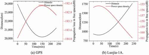
As can be seen from Figure 1, the distance from the ground station to the GNSS satellite and the distance to the Luojia-1A satellite are not of the same level. The large variation of the distance from the ground station to the Luojia-1A results in a larger range of free space propagation loss than that of GNSS, which should be taken into consideration when designing signal acquisition algorithms.

2.3. Large Doppler frequency shift range and high Doppler frequency shift rate

In satellite navigation and positioning, the Doppler effect is caused by the relative radial motion between the satellite and the receiver. Due to the Doppler effect, the frequency of the received carrier signal changes, limiting the length of the data used to capture the signal, increasing the complexity of signal acquisition. The frequency variation due to the Doppler effect is called the Doppler frequency shift. The Doppler frequency shift can be expressed by the following equation (Tsui 2005):

(4) $f_d=\frac{f{v}_d}{c}$(4)

where $f_d$ is the Doppler frequency shift; $f$ is the carrier frequency; $v_d$ is the relative radial speed between the receiver and the satellite; $c$ is the speed of light in vacuum. For GPS satellites, if the receiver is in a low-speed motion, the Doppler frequency shift is about 5 kHz; if the receiver is in high-speed motion, the Doppler frequency shift is about 10 kHz (Tsui 2005; Borre et al. 2007). In contrast to the GPS satellite, due to the fast geometry change of the Luojia-1A satellite, there is a large Doppler variation, which affects the signal acquisition efficiency (Wang et al. 2019). For the ground station, the radial velocity can be estimated by radial distance variation, and the equation is expressed as follows:

(5) $v_d=\frac{dr}{dt}$(5)

where $dr$ is the distance change from the ground station to the satellite during the time interval $dt$. The Doppler frequency shift and the Doppler frequency shift rate of the ground stationary station relative to the GPS satellite and the Luojia-1A satellite are calculated according to equations (4)(4) $f_d=\frac{f{v}_d}{c}$(4) and (5(5) $v_d=\frac{dr}{dt}$(5) ), respectively. The results are shown in Figure 2.

Figure 2. Doppler frequency shift and the Doppler frequency shift rate of the ground stationary station relative to the GPS satellite and the Luojia-1A satellite. (a) GPS. (b) Luojia-1A.

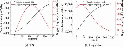
It can be seen from Figure 2 that the Doppler frequency shift and the Doppler frequency shift rate of the LEO satellite are much larger than those of the Medium Earth Orbit (MEO) satellite, which should be taken into consideration for the acquisition algorithm of the Luojia-1A satellite.

3. Methods

As can be seen from the previous section, the Doppler frequency shift range of the LEO satellite is large, and the rate of change of Doppler frequency shift rate is high. Therefore, a state-of-the-art parallel code-phase search acquisition algorithm is presented first. In addition, the variation of the power spatial density is also large according to the law of free space propagation of signals as demonstrated above. When the satellite is too far away from the ground station, the signal is too weak to acquire, so integration is adopted to improve the gain of the signal. Therefore, several major integration strategies are presented and compared to explore the signal acquisition effects of these methods on LEO navigation augmentation satellites such as the Luojia-1A satellite.

3.1. Parallel code phase search acquisition

Based on the implementation of code correlation and carrier correlation, there are three acquisition search algorithms: linear search, parallel frequency search, and parallel code-phase search. Parallel code-phase search, also called circular correlation search (Tsui 2005; Ziedan and Garrison 2004) can greatly reduce the computational burden and shorten the search time compared with the other two methods. All the acquisition algorithms implemented in this research are based on this search algorithm. The flow chart of the search algorithm is shown in Figure 3.

Figure 3. Flow chart of parallel code phase search acquisition.

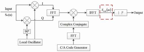
The algorithm only needs to perform an iterative search on the carrier frequency without iteration in the code phase. Moreover, the complex conjugate of the Fast Fourier Transform (FFT) of the C/A code can be generated in advance to speed up the search process. For the convenience of operation, input data of length 1 ms, corresponding to one code length, is adopted as a processing unit. The code-phase accuracy of the acquisition algorithm is related to the sampling rate of the data. The estimated code-phase error of 1 ms coherent integration does not exceed half a sampling interval, and for the data in this work, it does not exceed one-tenth of a chip length. The frequency search bandwidth is 500 Hz, and its estimation error is less than 250 Hz. The Doppler shift accuracy of the acquisition algorithm is related to the integration time of the acquisition algorithm, and the frequency search bandwidth is inversely proportional to the integration time. As the integration time $T$ increases, the frequency search bandwidth $f_{bin}$ shrinks, which can be simplified as $f_{bin}=500/T$.

For normal signal acquisition, the Inverse Fast Fourier Transform (IFFT) output of such a processing unit, the position at which the peak is obtained after modulo is the input signal code phase. However, for the acquisition of weak signals, it is difficult to complete the acquisition process by using only one processing unit, and it takes several processing units to complete the acquisition process. The dashed box in Figure 1 represents the operation for weak signal acquisition, and the IFFT output of each processing unit is adopted as an input to the operation. $S_{\mathrm{c}\mathrm{o}\mathrm{h}}\left(m\right)$ is the $m\mathrm{t}\mathrm{h}$ output or result of the processing unit. The operation for the acquisition of weak signals within the dashed box is described in detail below.

3.2. Strategies for weak signal acquisition

For unaided weak signal acquisition, the receiver sensitivity can be increased by extending the integration duration (Ziedan and Garrison 2004; Kong 2017). However, due to the bit transition and the high Doppler frequency shift rate of LEO, the integration duration cannot be extended indefinitely, and the integration acquisition process needs to be accomplished in as short a time as possible.

3.2.1. Non-coherent integration

Non-coherent integration is a method of increasing the signal-to-noise ratio gain by using the results of several successive processing units described in the previous section. The observation data for a long period is divided into several processing units and processed separately; then the absolute values of the processing results are accumulated as the detection value. The non-coherent operation is described by the following expression:

(6) $Ope{r}_{\mathrm{n}\mathrm{c}\mathrm{o}\mathrm{h}}\left(T_{\mathrm{u}\mathrm{n}\mathrm{i}\mathrm{t}},T_{\mathrm{n}\mathrm{c}\mathrm{o}\mathrm{h}}\right)=\sum _{m=1}^M\left|S_{\mathrm{c}\mathrm{o}\mathrm{h}}\left(m\right)\right|$(6)

where $M$ denotes the number of processing units, which is determined by the data length of a single processing unit $T_{\mathrm{u}\mathrm{n}\mathrm{i}\mathrm{t}}$ and the length of the entire integration $T_{\mathrm{n}\mathrm{c}\mathrm{o}\mathrm{h}}$. Since the non-coherent integration accumulates the absolute value of the result of each processing unit, it is less affected by the bit transition. Since the incoherent integration is little affected by the bit transition, the theoretical integration duration is not limited, but the non-coherent integration has a square loss, suppressing the signal-to-noise ratio gain of the weak signal (Xie 2009).

3.2.2. Coherent integration

The processing unit described above is a process of coherent integration with an integration duration of 1 ms. For longer coherent integration, a description similar to the non-coherent integration operation is as follows:

(7) $Ope{r}_{\mathrm{c}\mathrm{o}\mathrm{h}}\left(T_{\mathrm{u}\mathrm{n}\mathrm{i}\mathrm{t}},T_{\mathrm{n}\mathrm{c}\mathrm{o}\mathrm{h}}\right)=\left|\sum _{m=1}^M{S}_{\mathrm{c}\mathrm{o}\mathrm{h}}\left(m\right)\right|$(7)

where the meaning of the symbols in this expression is the same as the symbols in equation (6). The long-term observation data is divided into several processing units, which are processed separately; then the processing result is accumulated, and finally, the absolute value of the accumulated value is adopted as the detection value. However, unlike non-coherent integration, coherent integration acquisition may fail due to the bit transition. Therefore, variants of some coherent integration acquisition algorithms have emerged to eliminate or reduce the effects of bit transitions on coherent integration. Two improved algorithms based on the coherent integration acquisition algorithm are described the alternate half-bit method and the pre-guess test method.

As can be seen from the signal model introduced in the second section, the time interval at which bit transition occurs is a multiple of 20 ms. For a signal of 20 ms in succession, if a bit transition occurs in the first 10 ms, it is unlikely to occur in the last 10 ms. The alternate half-bit method is based on the above idea. First, the data need to be divided into several blocks at intervals of 10 ms. As shown in Figure 4, the entire data is divided into 2 n blocks. Then, a coherent integration is performed for each data block as described in equation (8)(8) $y_{\mathrm{b}\mathrm{l}\mathrm{o}\mathrm{c}\mathrm{k}}\left(i\right)=Ope{r}_{\mathrm{c}\mathrm{o}\mathrm{h}}\left(1\mathrm{m}\mathrm{s},10\mathrm{m}\mathrm{s}\right)\left(S_{\mathrm{b}\mathrm{l}\mathrm{o}\mathrm{c}\mathrm{k}}\left(i\right)\right)$(8) .

(8) $y_{\mathrm{b}\mathrm{l}\mathrm{o}\mathrm{c}\mathrm{k}}\left(i\right)=Ope{r}_{\mathrm{c}\mathrm{o}\mathrm{h}}\left(1\mathrm{m}\mathrm{s},10\mathrm{m}\mathrm{s}\right)\left(S_{\mathrm{b}\mathrm{l}\mathrm{o}\mathrm{c}\mathrm{k}}\left(i\right)\right)$(8)

Figure 4. Block division of the alternate half-bit method.

where the meaning of the symbols in this expression is the same as the symbols in equation (6); $S_{\mathrm{b}\mathrm{l}\mathrm{o}\mathrm{c}\mathrm{k}}\left(i\right)$ is the block divided as Figure 4, and $i=1,2,\dots 2n-1,2n$ is the index of the block; $y_{\mathrm{b}\mathrm{l}\mathrm{o}\mathrm{c}\mathrm{k}}\left(i\right)$ is the coherent integration of each block. For the above coherent integration results, according to the odd and even blocks, the non-coherent integration is performed separately, expressed as follows:

(9) $\left\{\begin{array}{c}{y}_{n\mathrm{c}\mathrm{o}\mathrm{h}-\mathrm{o}\mathrm{d}\mathrm{d}}=Ope{r}_{\mathrm{n}\mathrm{c}\mathrm{o}\mathrm{h}}\left(1\mathrm{m}\mathrm{s},10\mathrm{m}\mathrm{s}\right),\left(\mathrm{o}\mathrm{d}\mathrm{d}\mathrm{b}\mathrm{l}\mathrm{o}\mathrm{c}\mathrm{k}\mathrm{s}\right)\\ y_{\mathrm{n}\mathrm{c}\mathrm{o}\mathrm{h}-\mathrm{e}\mathrm{v}\mathrm{e}\mathrm{n}}=Ope{r}_{\mathrm{n}\mathrm{c}\mathrm{o}\mathrm{h}}\left(1\mathrm{m}\mathrm{s},10\mathrm{m}\mathrm{s}\right),\left(\mathrm{e}\mathrm{v}\mathrm{e}\mathrm{n}\mathrm{b}\mathrm{l}\mathrm{o}\mathrm{c}\mathrm{k}\mathrm{s}\right)\end{array}\right.$(9)

The non-coherent integration results $y_{\mathrm{n}\mathrm{c}\mathrm{o}\mathrm{h}-\mathrm{o}\mathrm{d}\mathrm{d}}$ are compared with $y_{\mathrm{n}\mathrm{c}\mathrm{o}\mathrm{h}-\mathrm{e}\mathrm{v}\mathrm{e}\mathrm{n}}$, where large results are free of bit transition and are adopted as the final detection value. This method can avoid the effect of bit transition, but the data utilization is only 50%, and the noise power is amplified in the non-coherent process.

The pre-guess test method is used to detect and handle the problem of bit transition unit by unit. Based on the existence and absence of a bit transition in the current processing unit, two coherent accumulating results are calculated, and the results are compared and determined for the following processing. The entire operation process is as follows:

(10) $Ope{r}_{\mathrm{g}\mathrm{u}\mathrm{e}\mathrm{s}\mathrm{s}}\left(T_{\mathrm{u}\mathrm{n}\mathrm{i}\mathrm{t}},T_{\mathrm{c}\mathrm{o}\mathrm{h}}\right)=\left|\sum _{m=1}^M\mathrm{s}\mathrm{i}\mathrm{g}\mathrm{n}\left(m\right)S_{\mathrm{c}\mathrm{o}\mathrm{h}}\left(m\right)\right|$(10)

where the meaning of symbols in this expression is the same as the symbols in (6); $\mathrm{s}\mathrm{i}\mathrm{g}\mathrm{n}\left(m\right)$ is the symbol, take +1 or -1, which can be determined by

(11) $\mathrm{i}\mathrm{g}\mathrm{n}\left(m\right)=\left\{\begin{array}{cc}+1,\left|\begin{array}{c}\sum _{n=1}^{m-1}\mathrm{s}\mathrm{i}\mathrm{g}\mathrm{n}\left(n\right)\\ S_{\mathrm{c}\mathrm{o}\mathrm{h}}\left(n\right)\\ +S_{\mathrm{c}\mathrm{o}\mathrm{h}}\left(m\right)\end{array}\right|>& \left|\begin{array}{c}\sum _{n=1}^{m-1}\mathrm{s}\mathrm{i}\mathrm{g}\mathrm{n}\left(n\right)\\ S_{\mathrm{c}\mathrm{o}\mathrm{h}}\left(n\right)\\ -S_{\mathrm{c}\mathrm{o}\mathrm{h}}\left(m\right)\end{array}\right|\\ -1,& otherwise\end{array}\right.$(11)

Since the problem of bit transition is considered in each processing unit, the influence of bit transition can be effectively eliminated incoherent integration. However, each processing unit adds additional accumulation and comparison operations, thus increasing the computation burden.

3.2.3. Differential coherent integration

There is also a technique called differential coherent integration that can take into account the advantages and disadvantages of the two methods mentioned above. In differential coherent integration, the processing results of adjacent processing units are conjugate multiplied, and the conjugate multiplication result is used as a new integral unit of coherent integration(Kong 2017; Xie 2009; Schmid and Neubauer 2004; Weixiao, Ruofei, and Shuai 2010). The operation is as follows:

(12) $Ope{r}_{\mathrm{d}\mathrm{i}\mathrm{f}\mathrm{f}}\left(T_{\mathrm{u}\mathrm{n}\mathrm{i}\mathrm{t}},T_{\mathrm{c}\mathrm{o}\mathrm{h}}\right)=\left|\sum _{m=1}^M{S}_{\mathrm{c}\mathrm{o}\mathrm{h}}^{\ast }\left(m-1\right)S_{\mathrm{c}\mathrm{o}\mathrm{h}}\left(m-1\right)\right|$(12)

where the meaning of symbols in this expression is the same as the symbols in (6). $S_{\mathrm{c}\mathrm{o}\mathrm{h}}^{\ast }\left(m-1\right)$ is the conjugate of $S_{\mathrm{c}\mathrm{o}\mathrm{h}}\left(m\right)$. This method, on the one hand, can reduce the square loss of non-coherent integration; on the other hand, the effect of the bit transition of traditional coherent integration can be mitigated.

3.3. Detection indicators

In the previous section, several integration strategies based on parallel code-phase search are introduced. To compare the effects of these integration processing strategies, appropriate detection indicators are selected in this section. To describe these detection indices uniformly, the correlation values of all searched grid points are given, and the expressions are denoted as $R\left(\delta f_i,\delta t_j\right)$, where $\delta f_i$ denotes the $i\mathrm{t}\mathrm{h}$ Doppler shift in the frequency search range; $\delta t_j$ denotes the $j\mathrm{t}\mathrm{h}$ code-phase delay in the code-phase search range.

3.3.1. Maximum-to-second-maximum ratio (MTSMR)

The ratio value between the maximum correlation value and the second maximum correlation value (MTSMR) is a widely used detection index in GNSS signal acquisition (Geiger, Vogel, and Soudan 2012; Kim and Kong 2014). The definition is as follows:

(13) ${\gamma }_{\mathrm{r}\mathrm{a}\mathrm{t}\mathrm{i}\mathrm{o}}=\frac{R_{\mathrm{m}\mathrm{a}\mathrm{x}}}{R_{\mathrm{s}\mathrm{u}\mathrm{b}}}$(13)

where $R_{\mathrm{m}\mathrm{a}\mathrm{x}}$ and $R_{\mathrm{s}\mathrm{u}\mathrm{b}}$ represent the maximum correlation value and the sub-maximum correlation value, respectively. The maximum correlation value $R_{\mathrm{m}\mathrm{a}\mathrm{x}}$ can be achieved by the following formula:

(14) $R_{\mathrm{m}\mathrm{a}\mathrm{x}}=R\left(\delta f_{i_{\mathrm{m}\mathrm{a}}},\delta t_{j_{\mathrm{m}\mathrm{a}}}\right)=max\left(R\left(\delta f_i,\delta t_j\right)\right)$(14)

where max is the maximum mathematical operator; $\delta f_{i_{\mathrm{m}\mathrm{a}}}$ and $\delta t_{j_{\mathrm{m}\mathrm{a}}}$ denote the Doppler frequency shift and code-phase delays at the maximum correlation value, $i_{\mathrm{m}\mathrm{a}\mathrm{x}}$ and $j_{\mathrm{m}\mathrm{a}\mathrm{x}}$ are the corresponding indexes of the search ranges. The second maximum correlation value $R_{\mathrm{s}\mathrm{u}\mathrm{b}}$ can be achieved as follows:

(15) $R_{\mathrm{s}\mathrm{u}\mathrm{b}}=\mathrm{m}\mathrm{a}\mathrm{x}\left(R\left(\delta f_{i_{\mathrm{m}\mathrm{a}}},\delta t_j\right)\right),j\notin \left[j_{\mathrm{m}\mathrm{a}\mathrm{x}}-l_{\mathrm{s}\mathrm{p}\mathrm{c}},j_{\mathrm{m}\mathrm{a}\mathrm{x}}+l_{\mathrm{s}\mathrm{p}\mathrm{c}}\right]$(15)

where $l_{\mathrm{s}\mathrm{p}\mathrm{c}}$ denotes the number of samples per code chip.

3.3.2. Maximum-to-mean ratio (MTMR)

The maximum-to-mean ratio is defined as follows:

(16) ${\gamma }_{\mathrm{m}\mathrm{m}}=\frac{R_{\mathrm{m}\mathrm{a}\mathrm{x}}}{R_{\mathrm{m}\mathrm{m}}}$(16)

where $R_{\mathrm{m}\mathrm{m}}$ is the mean of the correlation values, excluding the peak correlation value as well as the nearby correlation values, which can be achieved by the formula as follows:

(17) $\begin{array}{rl}& R_{\mathrm{m}\mathrm{m}}=\mathrm{m}\mathrm{e}\mathrm{a}\mathrm{n}\left(R\left(\delta f_i,\delta t_j\right)\right),i\notin \left[i_{\mathrm{m}\mathrm{a}\mathrm{x}}-1,i_{\mathrm{m}\mathrm{a}\mathrm{x}}+1\right]\\ & \mathrm{a}\mathrm{n}\mathrm{d}j\notin \left[j_{\mathrm{m}\mathrm{a}\mathrm{x}}-l_{\mathrm{s}\mathrm{p}\mathrm{c}},j_{\mathrm{m}\mathrm{a}\mathrm{x}}+l_{\mathrm{s}\mathrm{p}\mathrm{c}}\right]\end{array}$(17)

In this formula, the “mean” is the mean mathematical operator. It can be seen from the definition of maximum-to-mean ratio that it reflects the relative level between signal and noise from a statistical point of view. Under the conditions of the fixed signal system and integration length, different integration strategies will also affect the acquisition results. The effectiveness of these integration strategies in LEO satellite signal acquisition is presented below.

4. Experiments and results

To study the use of LEO for navigation enhancement, a series of experiments were conducted to collect the Luojia-1A satellite signal. At present, there is only one satellite of the Luojia series, namely the Luojia-1A test satellite. Due to the short transit time of the LEO satellite, all instruments were deployed ahead of time to wait for satellite transit. The experiment was carried out in an open sky environment, and experiments in complex environments will be carried out in the follow-up work.

4.1. Test bench for Luojia-1A signal sampling

In this work, a universal software radio peripheral (USRP) based test platform is designed for signal sampling and recording. USRP is an Ettus Research product, which is a low-cost, flexible, and tunable transceiver for designing, prototyping, and deploying radio communication systems. The USRP is designed to make ordinary computers work like high-bandwidth software radios. In the presented test bench, we use USRP X310, which has integrated a motherboard and two daughter boards. The USRP motherboard is responsible for clock generation and synchronization, digital-analog signal interface, host processor interface, and power management, while the USRP daughter board is used for up/down conversion, analog filtering, and other analog signals conditioning operations (Chen et al. 2015).

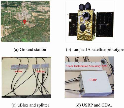
On 26 July 2019, data collected for about 8 mins was stored as a file, which serves as a data source for algorithm validation described in the previous section. In this way, the process of algorithm verification is greatly simplified. The experimental configuration is shown in Figure 5. The location of data collection is located at a ground station in Wuhan City as shown in subfigure (a) in Figure 5. The antenna used in the experiment is active, so an uBlox is connected to the splitter to power the antenna. The Clock Distribution Accessory 2990 (CDA-2990), also designed by Ettus Research, is an eight-channel clock distribution accessory for synchronizing multiple software radio systems and providing 1 pulse per second (PPS) time reference signals. The GPS Ant Input Interface of CDA-2990 is connected to the splitter. The frequency outputs are connected to different USRPs for device synchronization, and PPS outputs are connected to USRPs for timing. USRP interacts with the host computer through USRP Hardware Driver (UHD).

Figure 5. Experiment scene and configuration. (a) Ground station. (b) Luojia-1A satellite prototype. (c) uBlox and splitter. (d) USRP and CDA.

4.2. Results of process unit

To get the performance of the integration unit with an acquisition code length, that is, the acquisition effect of the processing unit mentioned above, the collected data is coherently integrated every 1 s, and the integration length is 1 ms. The acquisition results are shown in Figure 6.

Figure 6. Acquisition results of 1 ms coherent integration. Red: MTSMR value of each second; Green: the elevation angle of each second; Blue: the distance between the ground station and the satellite at each second.

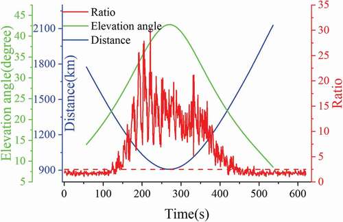
In Figure 6, the red, green, and blue lines represent MTSMR values, elevation angles, and distances between the ground station and the satellite, respectively. All these values are calculated every second. The red dashed line represents the MTSMR threshold, which is used to judge whether the acquisition is successful or not. Only signal acquisitions with a ratio value greater than this threshold are considered successful. In this paper, the MTSMR threshold is 2.5. From the above results, it can be concluded that with the increase in the distance between the station and the satellite, the elevation angle decreases, the ratio value decreases, and the acquisition results deteriorate. The total data time is about 10 mins, but the time interval to ensure successful acquisition is from 135 s to 419 s, a total of 285 s, less than 5 mins.

4.3 Results of 5 ms integration

Because the LEO transit time is very short, it is of great significance to expand the successful acquisition time range of the LEO navigation augmentation signal. In order to study the integration strategies for expanding the successful acquisition time range, different integration strategies are used for 5 ms integration. The ratio values acquired by different integration strategies and the acquired Doppler shift results are shown in Figure 7 and Figure 8, respectively.

Figure 7. Acquisition ratio value of 5 ms of different integration strategies.

(a) Overview of the acquisition ratio value. (b) Beginning of the acquisition ratio value. (c) End of the acquisition ratio value.

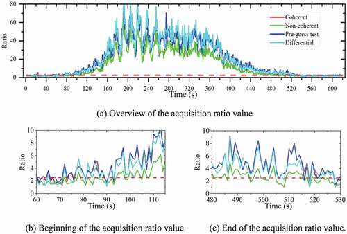
Figure 8. Doppler shift of 5 ms of different integration strategies.

(a) Overview of the Doppler shift. (b) Beginning of the Doppler shift. (c) End of the Doppler shift.

In Figure 7 and Figure 8, the red, green, blue, and cyan lines represent the acquisition results of coherent integration, non-coherent integration, pre-guess test integration, and differential coherent integration, respectively. All these values are calculated every second. Figure 7(a) and Figure 8(a) are overviews of the acquisition results of various integration strategies.

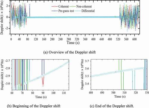
From Figure 7(b) and Figure 7(c), it can be concluded that the overall successful acquisition interval is from 94 s to 486 s, lasting 393 s. Compared with the result of the coherent integration of 1 ms, it has been greatly improved. To more finely present the available duration of acquisition under various integration strategies, the ratio values of transition time from available to unavailable and the corresponding Doppler shifts are presented in Figure 8(b) and Figure 8(c). By comparing Figure 7 and Figure 8, it can be found that some detection values are less than the ratio threshold, but the acquisition Doppler shift remains continuous. There is a misjudgment by setting the ratio threshold. Taking the results of incoherent integration as an example, although there are many ratio values below 2.5 between 91 seconds and 108 s, 486 s, and 505 s, the acquisition Doppler shift remains continuous and can be acquired correctly. The selection and setting of the threshold are discussed in the following section. It can be seen from the results of the acquired Doppler shift at 90 s, all methods except the differential coherence method fail. It can be seen from the results of the acquired Doppler shift in Figure 8(b) that at 505 s, all methods except the incoherent method are successfully acquired. It can be seen from the Doppler shift that the total available time is between 77 and 527 s, lasting 450 s.

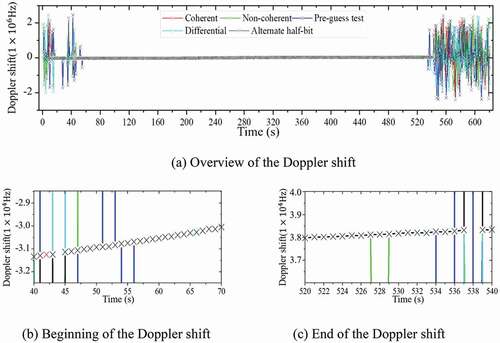
4.4. Results of 20 ms integration

The ratio and Doppler shift results of 20 ms integration are shown in Figure 9 and Figure 10, respectively. The integration results of the alternate half-bit method are also shown in figures. The display details in Figures 9, 10 are similar to those in Figures 7, 8, except that the newly added black element represents the result of the alternate half-bit method. As can be seen from these figures, the period during which the signal can be successfully acquired by the alternate half-bit method is from 45 s to 537 s. The alternating half-bit method acquired period coincides with the differential coherent acquired period. Due to the misjudgment of the bit transition, the performance of the pre-guess test is the worst. Similar to the 5 ms integration results, although some of the detected values are lower than the threshold of 2.5, the signal is successfully acquired, which is more obvious in the non-coherent integration.

Figure 9. Acquisition ratio value of 20 ms of different integration strategies. (a) Overview of the acquisition ratio value. (b) Beginning of the acquisition ratio value. (c) End of the acquisition ratio value.

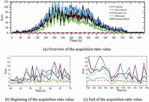
Figure 10. Doppler shift of 5 ms of different integration strategies. (a) Overview of the Doppler shift. (b) Beginning of the Doppler shift. (c) End of the Doppler shift.

4.5. Results of other integration duration

For different integration durations, the successful acquisition time length and range of different integration algorithms are summarized as shown in Table 1 and Figure 11. The successful acquisition time range is calculated based on the continuity of the Doppler shift. It can be seen from these results that the integration can effectively expand the range of successful acquisitions, thus increasing the available time of the signal. However, due to the influence of noise, the time range of successful acquisition will not expand infinitely with the increase in integration duration.

Figure 11. Successful acquisition time range of different integration algorithms for different integration duration lengths.

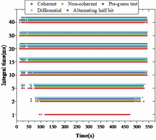
Table 1. Successful acquisition time lengths of different integration algorithms for different integration time lengths

Integration strategies	Coherent	Non-coherent	Pre-guess test	Differential	Alternating half bit
1 ms	327s
2 ms	393s	390s	393s	416s
5 ms	460s	445s	454s	465s
10 ms	510s	485s	482s	501s
15 ms	522s	495s	495s	513s
20 ms	522s	505s	502s	514s	514s
30 ms	509s	504s	505s	506s
40 ms	498s	493s	498s	494s	494s

5. Discussion

The above results show that the detection index is MTSMR, and the threshold of the detection index is an empirical value of 2.5. However, it can be found that the MTSMR output values of the different integration algorithms are significantly different, with the non-coherent MTSMR values being significantly smaller than the other integration strategies. At the same time, it is found that many MTSMR detection values are less than the threshold value, but the obtained Doppler shift remains continuous, that is, successfully obtained. Therefore, it is necessary to explore the reasonable setting of those indicators’ thresholds and whether those thresholds are related to the integration duration.

5.1. Thresholds of detection indicators

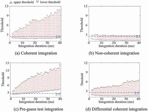
As shown in the previous section, the range of MTSMR detection value varies with different integration algorithms, such as the MTSMR detection value of non-coherent integration is significantly smaller than that of other integration algorithms. Based on the continuity of the Doppler shift, the probability of false alarm ($P_f$) using different MTSMR thresholds under different integration algorithms of 5 ms is given, as shown in Figure 12.

Figure 12. Probability of false alarm using different MTSMR thresholds under different integration algorithms of 5 ms. (a) Coherent integration. (b) Non-coherent integration. (c) Pre-guess test integration. (d) Differential coherent integration.

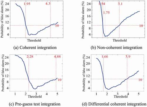
In Figure 12, the horizontal axis represents the threshold of MTSMR and the vertical axis represents the $P_f$. The horizontal red dot lines represent 10% $P_f$, and the vertical red dot lines represent the critical threshold for obtaining 10% $P_f$. Taking the non-coherent integration as an example, when the detection threshold of MTSMR is between 1.54 and 3.1, the non-coherent integration of 5 ms can achieve the $P_f$ less than 10%, that is, the probability of detection ($P_d$) is more than 90%. When the threshold is 1.75, the lowest $P_f$ value can be obtained: 2.7419%, that is, the $P_d$ reaches the maximum value: 97.2581%. If the threshold is set too large or too small, the $P_f$ will increase. When the threshold setting is too large, it is easy to detect a successful acquisition as a failed acquisition. When the threshold setting is too small, it is easy to detect a failed acquisition as a successful acquisition. To further discuss the relationship between the MTSMR threshold and the integration duration, the relationship between the integration duration and thresholds of less than 10% $P_f$ is given, as shown in Figure 13.

Figure 13. The upper and lower MTSMR thresholds of less than 10% $P_f$ for various integration duration. (a) Coherent integration. (b) Non-coherent integration. (c) Pre-guess test integration. (d) Differential coherent integration.

In Figure 13, the horizontal axis denotes the integration duration and the vertical axis represents the threshold of MTSMR. For coherent integration, non-coherent integration, and differential integration, the $P_f$ is less than 10% in the integration duration of 2–20 ms when the MTSMR threshold value is 2.5. For the pre-guess test integration, when the threshold is selected to be 2.5, the $P_f$ is greater than 10% when the integration duration is greater than 9 ms. Under the premise that the $P_f$ is less than 10%, with the prolongation of integration duration, the range of optional threshold of coherent integration increases gradually, the range of optional threshold of non-coherent integration is smaller and relatively stable, the range of optional threshold of pre-guess test gradually expands and tends to move upward, and the range of differential coherence threshold is relatively stable. For the other detection indicator MTMR mentioned above, the relationship between the integration duration and thresholds of less than 10% $P_f$ is also given as shown in Figure 14.

Figure 14. The upper and lower MTMR thresholds of less than 10% Pf for various integration duration. (a) Coherent integration. (b) Non-coherent integration. (c) Pre-guess test integration. (d) Differential coherent integration.

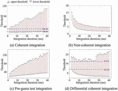
As can be seen from the figure, the obtained MTMR threshold range is significantly different in magnitude for different integration algorithms, so it is difficult to use a global value as the MTMR detection threshold for all integration algorithms. The threshold between two dot lines represents the intersection of the optional threshold ranges of different integration durations between 2 and 20 ms. Under the premise that the $P_f$ is lower than 10%, the lower limit of the optional threshold of coherent integration does not change significantly with the increase in the integration duration, and the overall range of the optional threshold increases with the upper limit of the threshold. The upper and lower limits of the optional thresholds of non-coherent integration gradually decrease, and the fluctuations are large. It is difficult to use the same threshold for non-coherent integrations to obtain less than 10% $P_f$ of different integration durations. The upper and lower limits of the optional thresholds of the pre-guess test method increase gradually, but the threshold range intersection of different integration durations is smaller. The lower limit of differential coherence the optional threshold decreases gradually and tends to be stable, and the range of optional threshold increases.

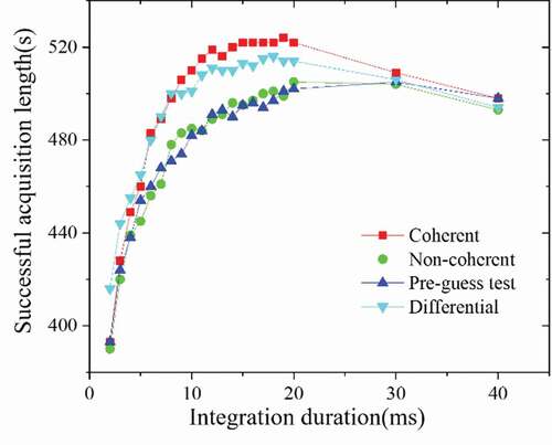
5.2. Integration duration

To study the relationship between integration duration and successful acquisition time, the acquisition time of 2–40 ms integration duration is calculated, which is shown in Figure 15. In general, with the increase in integration duration, the successful acquisition time first increases and then decreases, and the successful acquisition time will not increase indefinitely with the integration duration. When the integration duration is more than 20 ms, the length of successful acquisition time decreases. The effect of coherent integration and differential integration is better than the other two integration methods. When the integration duration is less than 9 ms, the effect of differential integration is better than that of coherent integration, and the effect of coherent integration is slightly better than that of coherent integration when the integration duration is longer than 9 ms.

Figure 15. Relationship between integration duration and successful acquisition time length.

6. Conclusions

This paper aims to study LEO signal acquisition and try to expand the successful acquisition time range. One of the most significant findings to emerge from this study is that the integration strategies expand the successful acquisition time range, and it will not expand indefinitely with the integration duration.

Through the study of LEO’s orbit and signal characteristics, it is found that compared with medium earth orbit satellites, LEO has the characteristics of large Doppler shift and large variation in power space density. Based on the parallel code search signal acquisition algorithm, the unified symbolic definitions of coherent integration, non-coherent integration, differential coherent integration, pre-guess test, and alternating half-bit algorithms are given. To verify and analyze the above acquisition algorithms, an SDR was developed and the real data were collected from the Luojia-1A satellite by using USRP. The experimental results show that the successful acquisition time range of the 1 ms integration duration is about 300 s. Integration strategies can significantly expand the successful acquisition time range, and the maximum acquisition time range can reach 522 s. However, due to the change in signal strength and the presence of bit transition, it is difficult to maintain a longer successful acquisition time range even if the integration duration is infinitely extended. In addition, the thresholds of detection indicators under different integration algorithms and various integration durations are discussed and given. For all integration algorithms except the pre-guess test, the $P_f$ is less than 10% in the integration duration of 2–40 ms when the MTSMR threshold value is adopted the empirical value 2.5 and it is difficult to use a global value as the MTMR detection threshold for all integration strategies. The trend of successful acquisition time range versus integration duration under different integration algorithms is discussed. The performance of coherent integration and differential integration is better than the other two integration algorithms. Therefore, coherent integration and differential integration algorithms are recommended, and a 20 ms integration duration is suggested.

Data availability statement

The data that support the findings of this study are available from the State Key Laboratory of Information Engineering in Surveying, Mapping and Remote Sensing (LIESMARS), www.lmars.whu.edu.cn. The University of Wuhan, but restrictions apply to the availability of these data, which were used under license for the current study, and so are not publicly available. Data are, however, available from the authors upon reasonable request and with permission of LIESMARS.

Additional information

Funding

This research was supported by the National Key R&D Program of China [grant number 2018YFB0505400] and the Natural Science Fund of Hubei Province with Project [grant number 2018CFA007];National Key Research and Development Program of China [2018YFB0505400];

Notes on contributors

Liang Chen

Liang Chen is a professor in the State Key Laboratory of Information Engineering in Surveying, Mapping and Remote Sensing, Wuhan University. His research interests include indoor positioning, wireless positioning, sensor fusion, and location-based services.

Xiangchen Lu

Xiangchen Lu is currently studying for a PhD in Geodesy at Wuhan University. His research direction is LEO navigation augmentation and software defined receiver.

Nan Shen

Nan Shen received a PhD degree from Wuhan University in 2021. His research interests focus on precise GNSS data processing, software defined receiver.

Lei Wang

Lei Wang is currently an associate research fellow at Wuhan University. He obtained a PhD degree from Queensland University of Technology, Australia in 2015. His research interest includes GNSS precise positioning, LEO navigation augmentation, LEO precise orbit determination, indoor positioning systems.

Yuan Zhuang

Yuan Zhuang is a professor at Wuhan University. His current research interests include multi-sensors integration, real-time location system, personal navigation system, wireless positioning, Internet of Things (IoT), and machine learning for navigation applications.

Ye Su

Ye Su is a masters student at Wuhan University. Her current research interests include outdoor positioning and V-SLAM.

Deren Li

Deren Li received the Dr. Eng. degree in photogrammetry and remote sensing from Stuttgart University, Stuttgart, Germany, in 1985. He was elected as an Academician of the Chinese Academy of Sciences, Beijing, China, in 1991, and the Chinese Academy of Engineering, Beijing, and the Euro–Asia Academy of Sciences, Beijing, in 1995. He was the President of the International Society for Photogrammetry and Remote Sensing Commissions III and VI and the first President of the Asia GIS Association, from 2002 to 2006. His research interests include spatial information science and technology, such as remote sensing, GPS and geographic information system (GIS), and their integration.

Ruizhi Chen

Ruizhi Chen is currently the director of LIESMARS. He was elected an Academician of Finnish Academy of Science and Letters in 2021. His main research interests include smartphone ubiquitous positioning and satellite navigation and positioning.

References

- Ardito, C. T., J. Morales, J. Khalife, A. Abdallah, and Z. Kassas. 2019. “Performance evaluation of navigation using LEO satellite signals with periodically transmitted satellite positions.” Proceedings of the 2019 International Technical Meeting of The Institute of Navigation, Virginia, USA, January 28-31.
- Borre, K., D. M. Akos, N. Bertelsen, P. Rinder, and S. H. Jensen. 2007. A software-defined GPS and Galileo receiver: A single-frequency approach. Boston: Birkhauser.
- Cao, Z., Y. Cheng, R. Chen, G. Guo, F. Ye, L. Chen, and Y. Pan. 2019. “An infant monitoring system with the support of accurate real-time indoor positioning.” Geo-spatial Information Science 22 (4): 1–11. doi:https://doi.org/10.1080/10095020.2019.1631617.
- Chen, L., O. Julien, P. Thevenon, D. Serant, A. G. Pena, and H. Kuusniemi. 2015. “TOA estimation for positioning with DVB-T signals in outdoor static tests.” IEEE Transactions on Broadcasting 61 (4): 625–638. doi:https://doi.org/10.1109/TBC.2015.2465155.
- Chen, L., R. Piche´, H. Kuusniemi, and R. Chen. 2014. “Adaptive mobile tracking in unknown non-line-of-sight conditions with application to digital TV networks.” EURASIP Journal on Advances in Signal Processing 2014 (1): 22. doi:https://doi.org/10.1186/1687-6180-2014-22.
- Chen, L., P. Thevenon, G. Seco-Granados, O. Julien, and H. Kuusniemi. 2016. “Analysis on the TOA tracking with DVB-T signals for positioning.” IEEE Transactions on Broadcasting 62 (4): 957–961. doi:https://doi.org/10.1109/TBC.2016.2606939.
- Chen, L., S. Thombre, K. Ja¨rvinen, E.S. Lohan, A. Ale´n-Savikko, H. Leppa¨koski, M. Z. H. Bhuiyan, S. Bu-Pasha, G. N. Ferrara, and S. Honkala. 2017a. “Robustness, security and privacy in location-based services for future IoT: A survey.” IEEE Access 5: 8956–8977. doi:https://doi.org/10.1109/ACCESS.2017.2695525.
- Chen, L., L.-L. Yang, J. Yan, and R. Chen. 2017b. “Joint wireless positioning and emitter identification in DVB-T single frequency networks.” IEEE Transactions on Broadcasting 63 (3): 577–582. doi:https://doi.org/10.1109/TBC.2017.2704422.
- Chen, R., and L. Chen. 2017. “Indoor Positioning with Smartphones: TheState-of-the-art and the Challenges.” Acta Geodaetica et Cartographica Sinica 46 (10): 1316–1326. doi:https://doi.org/10.11947/j.AGCS.2017.20170383.
- Chen, X., M. Wang, and L. Zhang. 2016. “Analysis on the performance bound of Doppler positioning using one LEO satellite.” 2016 IEEE 83rd Vehicular Technology Conference (VTC Spring), Nanjing, China, March 1, 1–5. doi:https://doi.org/10.1109/VTCSpring.2016.7504137.
- Dammann, A., R. Raulefs, and S. Zhang. 2015. “On prospects of positioning in 5G.” 2015 IEEE International Conference on Communication Workshop (ICCW), London, UK, 1207–1213. doi:https://doi.org/10.1109/ICCW.2015.7247342.
- Dangermond, J., and Michael F. Goodchild. 2020. “Building geospatial infrastructure.” Geo-spatial Information Science 23 (1): 1–9. doi:https://doi.org/10.1080/10095020.2019.1698274.
- Geiger, B. C., C. Vogel, and M. Soudan. 2012. “Comparison between ratio detection and threshold comparison for GNSS acquisition.” IEEE transactions on aerospace and electronic systems 48 (2): 1772–1779. doi:https://doi.org/10.1109/TAES.2012.6178098.
- Hofmann-Wellenhof, B., Herbert Lichtenegger Bernhard, and Elmar Wasle. 2007. GNSS–global navigation satellite systems: GPS, GLONASS, Galileo, and more. Vienna: Springer.
- Jia, Q., R. Wu, W. Wang, D. Lu, and L. Wang. 2018. “Adaptive blind anti-jamming algorithm using acquisition information to reduce the carrier phase bias.” GPS Solutions 22 (4): 99. doi:https://doi.org/10.1109/ACCESS.2017.2695525.
- Jin, S., E. Cardellach, and F. Xie. 2014. “GNSS Remote Sensing.” Springer EURASIP Journal on Advances in Signal Processing. doi:https://doi.org/10.1007/978-94-007-7482-7.
- Ke, M., J. Lv, J. Chang, W. Dai, K. Tong, and M. Zhu, 2015. “Integrating GPS and LEO to accelerate convergence time of precise point positioning.” 2015 International Conference on Wireless Communications & Signal Processing (WCSP), IEEE, Nanjing, China, October 15-17. doi:https://doi.org/10.1109/WCSP.2015.7341230.
- Khalife, J. J., and Z. M. Kassas, 2019. “Receiver design for Doppler positioning with LEO satellites.” ICASSP 2019-2019 IEEE International Conference on Acoustics, Speech, and Signal Processing (ICASSP), IEEE, Brighton, United Kingdom, May 12-17. doi:https://doi.org/10.1109/ICASSP.2019.8682554.
- Kim, B., and S.-H. Kong. 2014. “Determination of detection parameters on TDCC performance.” IEEE transactions on wireless communications 13 (5): 2422–2431. doi:https://doi.org/10.1109/TWC.2014.0204014.131704.
- Kong, S.-H. 2017. “High sensitivity and fast acquisition signal processing techniques for GNSS receivers: From fundamentals to state-of-the-art GNSS acquisition technologies.” IEEE Signal Processing Magazine 34 (5): 59–71. doi:https://doi.org/10.1109/MSP.2017.2714201.
- Li, D., Z. Shao, and R. Zhang. 2020. “Advances of geo-spatial intelligence at LIESMARS.” Geo-spatial Information Science 23 (1): 40–51. doi:https://doi.org/10.1080/10095020.2020.1718001.
- Li, D., X. Shen, D. Li, and S. Li. 2017. “On civil-military integrated space-based real-time information service system.” Geomatics and Information Science of Wuhan University 42: 1501–1505. doi:https://doi.org/10.13203/j.whugis20170227.
- Li, D., X. Zhao, and X. Li. 2016. “Remote sensing of human beings–a perspective from nighttime light.” Geo-spatial information science 19 (1): 69–79. doi:https://doi.org/10.1080/10095020.2016.1159389.
- Li, X., F. Ma, X. Li, H. Lv, L. Bian, Z. Jiang, and X. Zhang. 2019. “LEO constellation-augmented multi-GNSS for rapid PPP convergence.” Journal of Geodesy 93 (5): 749–764. doi:https://doi.org/10.1109/WCSP.2015.7341230.
- Lu, X., L. Chen, N. Shen, L. Wang, Z. Jiao, and R. Chen. 2021. “Decoding PPP Corrections From BDS B2b Signals Using a Software-Defined Receiver: An Initial Performance Evaluation.” IEEE Sensors Journal 21 (6): 7871–7883. doi:https://doi.org/10.1109/JSEN.2020.3041486.
- Misra, P., and P. Enge. 2006. Global positioning system: Signals, measurements and performance. Second ed. Massachusetts: Ganga-Jamuna Press.
- Schmid, A., and A. Neubauer, 2004. “Performance evaluation of differential correlation for single shot measurement positioning.” Proceedings of the 17th International Technical Meeting of the Satellite Division of the Institute of Navigation (ION GNSS 2004), CA, USA, September 21-24, 1998–2009. doi:https://doi.org/10.1080/135103404200317761.
- Shen, N., L. Chen, J. Liu, L. Wang, T. Tao, D. Wu, and R. Chen. 2019. “A Review of Global Navigation Satellite System (GNSS)-based Dynamic Monitoring Technologies for Structural Health Monitoring.” Remote Sensing 11 (9): 1001. doi:https://doi.org/10.3390/rs11091001.
- Shen, N., L. Chen, L. Wang, H. Hu, X. Lu, C. Qian, J. Liu, S. Jin, and R. Chen. 2021. “Short-Term Landslide Displacement Detection Based on GNSS Real-Time Kinematic Positioning.” IEEE Transactions on Instrumentation and Measurement 70: 1–14. doi:https://doi.org/10.1109/TIM.2021.3055278.
- Shen, N., L. Chen, L. Wang, X. Lu, T. Tao, J. Yan, and R. Chen. 2020. “Site-specific real-time GPS multipath mitigation based on coordinate time series window matching.” GPS Solutions 24 (3): 1–14. doi:https://doi.org/10.1007/s10291-020-00994-z.
- Ta, T.H., S.U. Qaisar, A. G. Dempster, and F. Dovis. 2021. “Partial differential postcorrelation processing for GPS L2C signal acquisition.” IEEE Transactions on Aerospace and Electronic Systems 48 (2): 1287–1305. doi:https://doi.org/10.1109/TAES.2012.6178062.
- Trinder, J., and Qingxiang Liu. 2020. “Assessing environmental impacts of urban growth using remote sensing.” Geo-spatial Information Science 23 (1): 20–39. doi:https://doi.org/10.1080/10095020.2019.1710438.
- Tsui, J. B.-Y. 2005. Fundamentals of global positioning system receivers: A software approach. New Jersey: John Wiley & Sons.
- Wang, L., R. Chen, D. Li, B. Yu, and C. Wu. 2018a. “Quality assessment of the LEO navigation augmentation signals from Luojia-1A satellite.” Geomatics and Information Science of Wuhan University 43: 2191–2196. doi:https://doi.org/10.13203/j.whugis20180413.
- Wang, L., R. Chen, D. Li, G. Zhang, X. Shen, B. Yu, C. Wu, S. Xie, P. Zhang, and M. Li. 2018b. “Initial assessment of the LEO based navigation signal augmentation system from Luojia-1A satellite.” Sensors 18 (11): 3919. doi:https://doi.org/10.3390/s18113919.
- Wang, L., R. Chen, B. Xu, X. Zhang, T. Li, and C. Wu. 2019. “The challenges of LEO based navigation augmentation system–lessons learned from Luojia-1A satellite.” China Satellite Navigation Conference, Springer, Beijing, China, May 22-25, 298–310. doi:https://doi.org/10.1007/978-981-13-7759-4_27.
- Wang, Y., L. Chen, P. Wei, and X. Lu. 2020. “Visual-Inertial Odometry of Smartphone under Manhattan World.” Remote Sensing 12 (22): 3818. doi:https://doi.org/10.3390/rs12223818.
- Weixiao, M., M. Ruofei, and H. Shuai, 2010. “Optimum path based differential coherent integration algorithm for GPS C/A code acquisition under weak signal environment.” IEEE 2010 First International Conference on Pervasive Computing, Signal Processing and Applications, Harbin, China, September 17-19. doi:https://doi.org/10.1109/PCSPA.2010.295.
- Wymeersch, H., G. Seco-Granados, G. Destino, D. Dardari, and F. Tufvesson. 2017. “5G mmWave positioning for vehicular networks.” IEEE Wireless Communications 24 (6): 80–86. doi:https://doi.org/10.1109/MWC.2017.1600374.
- Xie, G. 2009. Principles of GPS and receiver design. Beijing: Electronic Industry Press.
- Yan, J., Y. Cao, B. Kang, X. Wu, and L. Chen. 2021. “An ELM-Based Semi-Supervised Indoor Localization Technique With Clustering Analysis and Feature Extraction.” IEEE Sensors Journal 21 (3): 3635–3644. doi:https://doi.org/10.1109/JSEN.2020.3028579.
- Yan, J., K. Yu, R. Chen, and L. Chen. 2017. “An Improved Compressive Sensing and Received Signal Strength-Based Target Localization Algorithm with Unknown Target Population for Wireless Local Area Networks.” Sensors 17 (6): 1246. doi:https://doi.org/10.3390/s17061246.
- Yan, J., L. Zhao, J. Tang, Y. Chen, R. Chen, and L. Chen. 2018. “Hybrid Kernel Based Machine Learning Using Received Signal Strength Measurements for Indoor Localization.” IEEE Transactions on Vehicular Technology 67 (3): 2824–2829. doi:https://doi.org/10.1109/TVT.2017.2774103.
- Zhou, X., L. Chen, J. Yan, and R. Chen. 2020. “Accurate DOA Estimation With Adjacent Angle Power Difference for Indoor Localization.” IEEE Access 8: 44702–44713. doi:https://doi.org/10.1109/ACCESS.2020.2977371.
- Ziedan, N. I., and J. L. Garrison. 2004. “Unaided acquisition of weak GPS signals using circular correlation or double-block zero padding.” Position Location and Navigation Symposium (IEEE Cat. No. 04CH37556), IEEE, CA, USA, April 26-29. doi:https://doi.org/10.1109/PLANS.2004.1309030.