i4sea: a big data platform for sea area monitoring and analysis of fishing vessels activity

ABSTRACT

The i4sea research project provides effective and efficient big data integration, processing, and analysis technologies to deliver both real-time and historical operational snapshots of fishing vessels activity in national sea areas. This paper presents the architecture of the i4sea big data platform for sea area monitoring and analysis of fishing vessels activity and demonstrates the operation of some use-case pilot scenarios.

KEYWORDS:

• Big data
• fishing
• vessel activity
• machine learning

1. Introduction

Sea area monitoring is a critical tool to protect maritime resources, track and surveil sea vessels activity, and optimize supply chains for marine economy. Marine traffic data play a key role in sea area monitoring. Examples include VMS (Vessel Monitoring Systems) and AIS (Automatic Identification System) data. Both are widely used in Monitoring Control and Surveillance (MCS) programs at national and international levels. VMS are digital systems used in commercial fishing to allow regulatory organizations to track and monitor the activities of fishing vessels. The aim is to improve the management and sustainability of the marine environment by ensuring proper fishing practices and preventing illegal fishing. Other sources of valuable data are, meteorological (e.g. precipitation and wind speed), environmental (e.g. sea temperature and chlorophyll levels) and geographical (e.g. coastline and bathymetry) data.

There exist several commercial software¹ that provide monitoring functionality for fishing vessels activity, by utilizing VMS data. However, VMS data have a low sampling rate (approximately 1 message every 15 minutes) and often transmit inaccurate and incomplete identification and activity data. For this reason, we claim that combining VMS data with other sources of vessel traffic data, e.g. AIS (2 seconds to 3 minutes per message), will improve their accuracy and their quality (Veracity). Moreover, effectively supporting maritime surveillance requires, in addition to traffic data, the combined use of geographical, meteorological, and environmental data that (a) will improve the accuracy of identification operations, and (b) better support the export of mobility behavior patterns (Variety). Furthermore, simply monitoring the fishing vessels activity is not enough for a system that targets to protect maritime resources and optimize supply chains for marine economy. For this reason, such a system should also be able to support analysis of such data, such as pattern detection and predictive analytics, both in an offline and online manner. Finally, the creation of an effective “operational image” (real time and historical) of surveillance of marine areas requires enormous amounts of both static and streaming data (Volume and Veracity). Motivated by the above, our goal is to build an innovative Big Data system that will be able to efficiently collect, manage, and analyze, both in an offline and online fashion, large volumes of incoming marine surveillance data along with other contextual data, such as meteorological and environmental. Furthermore, we aim to further extend and integrate already developed data processing techniques and to develop innovative Big Data Analytics solutions.

Several real-life application scenarios could benefit from such a system. For example, detecting and/or predicting, in real time, illegal activities, such as illegal fishing, illegal transshipment, and trespassing in forbidden zones. The detection can be achieved by utilizing the incoming stream of traffic data along with other contextual information, such as fishing zones or forbidden zones (e.g. Natura 2000 zones). The prediction can be achieved by employing historical information in order to build a predictive model and utilize this predictor in order to predict the future movement of fishing vessels. Another interesting scenario is the estimation and/or the prediction of fishing pressure. Moreover, a common functionality of such systems is the polling procedure, where a user/controller sends a POLL request (position/status signal request) in order to identify fishing vessels that are about to present some kind of deviating behavior. What would be of great interest, is if the system could indicate a subset of vessels for which there is a high probability of delinquent behavior in the near future. Finally, we could avoid firing false alarms for illegal fishing activity, by taking into account real-time wind data and related traffic data, in order to better estimate vessel activity and verify routes.

While state-of-the-art technologies to collect, store, and analyze marine traffic data are mature enough to provide efficient and effective solutions, providing an integrated solution to the problem of monitoring and analyzing fishing vessels activity both in an online and offline manner is a challenging task. More specifically, different components have to be seamlessly integrated under an appropriate system architecture and several offline and online analytic techniques, tailored to fishing vessels activity, have to be devised and implemented. Apart from the commercial software that we already mentioned, there are several research projects that deal with similar challenges (AMINESS Project; BlueBRIDGE Project; DatAcron Project; FERARI Project; INFORE Project) in the maritime domain. However, these efforts do not focus specifically in monitoring and analyzing fishing vessels activity.

In this paper, we propose the i4sea Big Data platform (i4sea project) which aims at sea area monitoring and analysis tailored to fishing vessels activity. The vision is to provide effective and efficient big data integration, processing and analysis technologies to deliver both real-time and historical operational snapshots of fishing vessels activity in national sea areas. The key objectives are as follows:

• Propose an architecture that enables different modules and technologies to interact seamlessly, in a plug-and-play manner, and facilitates access to batch processing and stream processing methods in a hybrid manner.

• Enhance the value of vessel traffic data through the integration with open geographic, environmental, and meteorological data.

• Effective support for behavioral analysis and extraction of navigation patterns from historical vessel activity data, in conjunction with geographic, environmental, and meteorological parameters.

• Support of activity detection and prediction techniques through the real-time, online analysis of the incoming streams of data.

The platform will be tested in real use-case scenarios provided by COSMOS S.A., which operates the Sea Observer VMS IT infrastructure for the Hellenic Fish-Breeding Center (EHINAP²) to monitor fishing activity in Greece.

This paper presents the architecture of the i4sea big data platform for sea area monitoring and analysis of fishing vessels activity and demonstrates the operation of some use-case pilot scenarios. To the best of our knowledge, this is the first system that deals with the problem of sea area monitoring and analysis of fishing vessels activity in the era of Big Data.

2. Related work

2.1. Research projects

The INFORE Project addresses the challenges posed by huge datasets and real-time, interactive extreme-scale analytics and forecasting, among others, for maritime surveillance applications. DatAcron (DatAcron Project) addresses requirements from the air-traffic management and maritime domains by developing advanced tools for detecting and visualizing threats, abnormal activity, increasing the safety and efficiency of operations related to vessels and airplanes. BlueBRIDGE (BlueBRIDGE Project) develops smart solutions to support decision-makers involved in the fisheries and aquaculture ecosystem by facilitating the knowledge production chain (data collection, aggregation, analysis, and the production of indicators for authorities and investors). FERARI (FERARI Project) focuses on big data architecture for complex event detection and monitoring large data streams. Finally, AMINESS (AMINESS Project) promotes shipping safety in the Aegean Sea through a web portal offering different levels of access to relevant stakeholders such as shipowners, policymakers, the scientific community, and the general public. However, all of the above efforts do not focus specifically in fishing vessels activity. The i4sea project (Big Data in Monitoring and Analyzing Sea Area Traffic: innovative ICT and analysis models) (i4sea project; Tampakis 2020) will design and develop an innovative big data platform for sea area monitoring and analysis tailored to fishing vessels activity. The vision of the project is to provide effective and efficient big data integration, processing and analysis technologies to deliver both real-time and historical operational snapshots of fishing vessels activity in national sea areas.

2.2. Analytics

2.2.1. Trajectory joins

An important operation, which is the cornerstone of several knowledge discovery techniques from mobility data is the so-called trajectory join problem. There are a lot of efforts that try to deal with the problem of trajectory join in a centralized way (Bakalov et al. 2005, 15; Chen and Patel 2009). However, all of the above approaches are centralized and applying them to a parallel and distributed environment is non-trivial. Toward this direction, there is a bunch of research efforts that try to tackle this problem in a distributed setting (Fang et al. 2016; Shang et al. 2017, 2018; Xie, Li, and Phillips 2017; Zeinalipour-Yazti, Lin, and Gunopulos 2006). However, the definitions of these works are rather limited since they return pairs of trajectory ids that satisfy the join predicate but not the actual portion of these trajectories. To deal with this, the authors in Tampakis et al. (2020) introduce an efficient and highly scalable approach to deal with the distributed subtrajectory join problem, by means of MapReduce. More specifically, they try to identify all pairs of subtrajectories that move “close enough” in time and space w.r.t. a spatial threshold ${\epsilon }_{\mathit{sp}}$ and a temporal tolerance ${\epsilon }_t$ and is comprised of a Repartitioning phase and a Query phase.

2.2.2. Co-movement patterns

This line of research aims to identify several types of collective behavior patterns among moving objects. One of the first approaches for identifying such collective mobility behavior is the so-called flock pattern (Laube, Imfeld, and Weibel 2005; Vieira, Bakalov, and Tsotras 2009), which identifies groups of at least $\mathit{m}$ objects that move within a disk of radius $\mathit{r}$ for at least $\mathit{k}$ consecutive timepoints. Inspired by this, a less “strict” definition of flocks was proposed in Kalnis, Mamoulis, and Bakiras (2005) where the notion of a moving cluster was introduced. There are several related works that emerged from the above ideas, like the approaches of convoys (Jeung et al. 2008; Orakzai, Calders, and Pedersen 2019), swarms (Li et al. 2010), platoons (Li, Bailey, and Kulik 2015), traveling companion (Tang et al. 2012) and gathering pattern (Zheng et al. 2013). Recently, Tritsarolis, Theodoropoulos, and Theodoridis (2020) propose a novel co-movement pattern definition, called evolving clusters, that unifies the definitions of flocks and convoys and reduces them to Maximal Cliques (MC), and Connected Components (MCS), respectively. In addition, the authors propose an online algorithm, that discovers several evolving cluster types simultaneously in real time using Apache Kafka, without assuming temporal alignment, in contrast to the seminal works (i.e. flocks and convoys).

2.2.3. Trajectory clustering

Another line of research tries to discover groups of either entire or portions of trajectories considering their routes. There are several approaches whose goal is to group whole trajectories, including T-OPTICS (Nanni and Pedreschi 2006; Pelekis et al. 2016), that incorporates a trajectory similarity function into the OPTICS algorithm. However, discovering clusters of complete trajectories can overlook significant patterns that might exist only for portions of their lifespan. To deal with this, another line of research has emerged, that of Subtrajectory Clustering (Pelekis et al. 2017a, Pelekis, et al., 2017b; Tampakis et al. 2018, 2019), where the goal is to partition a trajectory into subtrajectories, whenever the density or the composition and its neighborhood changes “significantly,” then form groups of similar ones, while, at the same time, separate the ones that fit into no group, called outliers.

2.2.4. Hot-spot analysis

Hot-spot analysis aims at discovering statistically significant clusters. Spatial statistics were used in Moran (1950) and Ord and Getis (1995) while the spatio-temporal case has been studied in Hong et al. (2015) and Lukasczyk et al. (2015). Furthermore, efficient parallel hot-spot analysis algorithms on point spatio-temporal hot-spots are proposed in Makrai, 2016 and Nikitopoulos et al. (2016). Recently, in Nikitopoulos et al. (2018) statistics were used to discover hot-spots on trajectory data.

2.2.5. Future Location Prediction

The fact that the Future Location Prediction (FLP) problem has been extensively studied brings up its importance and applicability in a wide range of applications. Toward tackling the FLP problem, on line of work includes efforts that take advantage of historical movement patterns in order to predict the future location. Such an approach is presented in Trasarti et al. (2017), where the authors propose MyWay, a hybrid, pattern-based approach that utilizes individual patterns when available, and when not, collective ones, in order to provide more accurate predictions and increase the predictive ability of the system. In another effort, Petrou et al. (2019) utilize the work done by Tampakis et al. (2019) on distributed subtrajectory clustering in order to be able to extract individual subtrajectory patterns from big mobility data. These patterns are subsequently utilized in order to predict the future location of the moving objects in parallel.

A different way of addressing the FLP problem includes machine learning approaches. Valsamis et al. (2017) model the trajectory of sea vessels and provide a service that predicts in near-real time the position of any given vessel by employing multilayer perceptrons (MLPs). Zorbas et al. (2015) introduce a machine-learning model which exploits geospatial time-series surveillance data generated by sea-vessels, to predict future trajectories based on real-time criteria. Several different machine-learning algorithms were tested in terms of regression accuracy, as measured by means absolute error, and execution time. The perceptron was selected as it outperformed all other algorithms. Park et al. (2018) propose a prediction technique which can generate the future trajectory sequence of surrounding vehicles in real time by employing sequence-to-sequence LSTM encoder-decoder architecture. (Anagnostopoulos, Anagnostopoulos, and Hadjiefthymiades 2011) treat the FLP problem as a classification problem through the adoption of machine learning techniques, such as C4.5.

3. Architecture

3.1. Overview

To deal with the big data available for i4sea’s use case scenarios and to support arbitrary processing and analysis functions, we follow a lambda architecture that facilitates access to batch processing and stream processing methods in a hybrid manner. The aim of such an approach is to balance latency, throughput, and fault-tolerance. This is achieved by using batch processing for comprehensive views of historical data, while simultaneously using stream processing to provide views of real-time data. The two views may be joined before presentation.

The overall architecture of the i4sea big data platform is illustrated in Figure 1. More specifically, the architecture is based on six modules, where both batch and streaming data are managed and exploited in order to achieve the goals of surveillance of marine areas and analysis of vessel traffic. The data entry point for the platform is the Data Manager, which collects, pre-processes, fuses, and enriches the incoming data. The output of the Data Manager is written to some persistent storage and is also fed to subsequent modules that perform online analytics. The Storage Layer is responsible for storing the produced data. The Offline Analytics module is responsible for performing the required batch analytics. Data produced from this module is stored to the Storage Layer and can be subsequently utilized by several online analytics. The Online Analytics module receives input from the incoming streams produced by the Data Manager and the Storage Layer, where results of the Offline Analytics are stored. Finally, the Application Layer module consists of several applications that utilize the i4sea platform in order to model fleet dynamics, estimate fishing pressure, identify and predict vessel activities, etc. The Application Layer includes visualization methods responsible for visualizing data as required by the different application scenarios.

Figure 1. Overall architecture.

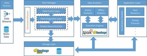
All these modules play a significant and necessary role toward the achievement of applications’ requirements. More specifically, an important goal of the i4sea platform is the integration and fusion of data sources, which aims at the integration of mobility data of vessels with sources of open geographical, environmental, and meteorological data and the fusion of traffic data from different data sources (VMS and AIS data) that correspond to the same entities (vessels). An additional goal is to design and implement methods for compression, extraction of synopses and detection of semantically enriched trajectories from multiple streams of real-time traffic data. Both of these application requirements are implemented inside the Data Manager Layer. Moreover, an important goal of the i4sea platform is the analysis of combined traffic data, which aims to develop methods and tools for data analysis from streams and historical vessel traffic data. Furthermore, another important goal is the prediction of fishing vessels traffic and activities, which aims at the design and development of algorithms for long-term prediction of (a) location, (b) itineraries, and (c) fishing vessels activities. These application requirements are realized inside the Data Analytics Module (Offline and Online). Finally, another key application requirement is the Fleet dynamics modeling, which aims at the implementation of fleet dynamics modeling methodologies and the Fishing Pressure Estimation. Both of these use case scenarios are implemented through the Application Layer.

In general, we utilized several “out of the box” Big Data solutions, which depend on commodity machines and do not require any special hardware. These solutions are seamlessly integrated and provide the opportunity both for offline and online analytics, through a simple lambda architecture. The backbone of the i4sea platform, which enables the different modules and technologies to interact seamlessly, is the coordination and communication system. To achieve this, we employed Kafka (Kreps, Narkhede, and Rao 2011), a state-of-the-art publish-subscribe messaging system that facilitates both the management and processing of streaming data.

3.2. Data manager

One of the main objectives of this module is data collection. The available data sources include:

• streaming sources, such as mobility data (VMS and AIS),

• dynamic sources, updated daily or annually, such as weather data and environmental data (e.g. chlorophyll levels)

• static sources, such as geospatial data (e.g. bathymetry, coastline, and protected areas).

The Data Manager is responsible for fusing incoming streams of traffic data from different data sources (VMS and AIS data) that correspond to the same entities (vessels). Furthermore, the Data Manager handles the integration of traffic data with other sources, such as weather or environmental data, thus resulting in multiple enriched streams that can be either stored or read by other modules and applications in a publish-subscribe fashion through Kafka Topics.

3.3. Storage layer

The Storage Layer is designed to accumulate immense volumes of historical data as the incoming streams of data arrive, and store data produced from other modules that might be useful in the future. Toward this direction, the platform utilizes the Hadoop Distributed File System (HDFS) (Shvachko et al. 2010), which is able to store in a scalable, durable and fault tolerant way enormous volumes of data. Furthermore, this module should be able to facilitate efficient retrieval of data, as required by several tasks of the Offline and Online Analytics module. To tackle this specification, we utilized Elasticsearch (Gormley and Tong 2015) that allows for the efficient retrieval of data in near real-time.

3.4. Offline analytics

This module is responsible for analyzing large volumes of historical data and extracting useful knowledge out of them, which can be subsequently utilized either by the Online Analytics module or by the end-applications. In order to achieve this, the different offline analytic processes access the data either directly from the Storage Layer. To support big data batch processing, we employed state-of-the-art batch processing solutions: Hadoop (Shvachko et al. 2010) and Spark (Zaharia et al. 2016). Examples of such offline analytic processes are presented in (Tampakis et al. 2020), where methods to identify all pairs of moving objects that moved “close” enough in space and time for at least some duration are presented, and in (Tampakis et al. 2019) which identifies clusters of vessel sub-trajectories.

3.5. Online analytics

The goal of this module is to be able to perform analytics over the incoming streams. The input data is the data streams produced by the Data Manager, and the offline analytic processes, through Kafka Topics and HDFS, respectively. This module should be able to perform streaming or micro-batch processing over high velocity incoming streams. To achieve this, we utilize Spark Streaming (Armbrust et al. 2018) and Kafka (Kreps, Narkhede, and Rao 2011) (more specifically the KafkaConsumer interface). More specifically, Spark Streaming is used for micro-batch analytic tasks and Kafka is utilized for tasks that require operational latency (response time in the order of milliseconds). Examples of such online processes are as follows: future location prediction, vessel activity prediction, etc.

3.6. Application Layer

The Application Layer module consists of the set of applications that conform to the specifications set by business cases. The input of this module comes from all the offline and online analytics along with contextual data stored in the Storage Layer. According to each business case requirement, the different components are combined together appropriately in order to produce the desired result.

The Application Layer also includes components that can help developers build applications on top of the platform. One such component is a deployment of the web-based notebook, Apache Zeppelin. It has great support for Spark in particular, including language backends for Java, Scala, Python, and R. Apache Zeppelin also provides tools for big data visualization, as well as the results of batch analysis performed by applications, with support for charts and maps for geospatial data. The architecture modules are available to Apache Zeppelin in the form of software libraries that expose reusable methods and APIs that can be combined for specific use cases. Users of the platform can create notebooks in Apache Zeppelin, while having access to the functionalities provided by the data manager, storage layer, and analytics modules of the platform.

4. Data preparation

4.1. Data fusion

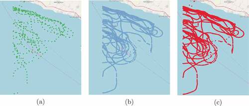
One of the main of objectives of i4sea platform is to combine heterogenous data (e.g. mobility traces and weather), as well as homogenous data, in order to produce value for the end-user. Combining homogenous data is actually the “fusion” of incoming streams of data from different sources, that represent the same entities. In our case, we have two alternative sources of mobility data, namely VMS and AIS data. VMS data are produced by the vessel monitoring system, which is a satellite-based monitoring system which at regular intervals provides data to the fisheries authorities on the location, course and speed of vessels. An example of such a vessel is illustrated in Figure 2(a). This data can be subsequently joined with static data sources and get enriched with valuable information, such as the type of the fishing vessel and the kind of gear that it carries. On the downside, VMS data have an increased reporting period, approximately 1 message every 15 minutes, due to the increased message cost, originating from the fact that VMS is a satellite-based system. This fact can introduce a lot of uncertainty in the i4sea system, since it will be unaware of the movement of a fishing vessel in between the received messages. On the other hand, AIS data is a low-cost automatic tracking system that uses transponders on vessels and base stations through the VHS frequency. Due to this fact, AIS data have a significantly lower reporting period (2 seconds to 3 minutes per message), as depicted in Figure 2(b), than VMS data and could be used to “enhance” VMS traces with extra mobility information, in the cases where a fishing vessel is equipped with both VMS and AIS systems, as illustrated in Figure 2(c). However, a significant problem during this procedure is that there is no matching id in order to perform this join between AIS and VMS.

Figure 2. The (a) VMS trace, (b) AIS trace and (c) Fused trace of a specific fishing vessel.

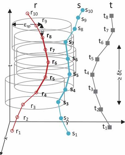
For this reason, we tried to exploit the spatiotemporal information provided by the two sources. In order to achieve this, we built upon the Distributed Subtrajectory Join solution proposed in (Tampakis et al. 2020), which given two sets of trajectories (or a single set and its mirror in the case of self-join), identifies all pairs of maximal “portions” of trajectories (or else, subtrajectories) that move close in time and space w.r.t. a spatial threshold ${\epsilon }_{\mathit{sp}}$ and a temporal tolerance ${\epsilon }_t$, for at least some time duration $\mathit{\delta t}$. Furthermore, we utilized the trajectory similarity function introduced in (Tampakis et al. 2019), which is a variation of the LCSS similarity between trajectories, that incorporates the distance proportionality, in order to implement a scalable and efficient solution to the Distributed Most Similar Trajectory Join query (DMSTJ).³

Definition 4.1. Given two sets of trajectories $\mathit{R}$ and $\mathit{S}$, $\mathrm{\forall }$ trajectory $\mathit{r}\in \mathit{R}$, we want to discover the most similar trajectory $\mathit{s}{ }^{\mathrm{\prime }}\in \mathit{S}$ for which it holds that $\mathit{Sim}(\mathit{r},\mathit{s}{ }^{\mathrm{\prime }})>\mathit{\alpha }$ and $\mathrm{\forall }$ trajectory $\mathit{s}\in \mathit{S}$ the goal is to discover the most similar trajectory $\mathit{r}{ }^{\mathrm{\prime }}\in \mathit{R}$ for which it holds that $\mathit{Sim}(\mathit{s},\mathit{r}{ }^{\mathrm{\prime }})>\mathit{\alpha }$, where $\mathit{\alpha }$ is a similarity threshold.

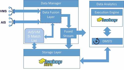
In more detail, as depicted in Figure 3, the AIS/VMS fusion procedure consists of an offline and an online module. In the offline module, the DMSTJ query runs periodically over the accumulated data and updates the AIS/VMS Match List. During the online module, the system utilizes this list in order to fuse appropriately the incoming VMS and AIS streams.

Figure 3. Overall architecture.

4.2. Noise Elimination and Synopses Generation

An important step when dealing with streams of mobility data is to cope with data stream imperfections, such as the inherent noise in vessel positions due to sea drift, discrepancies in GPS signals, etc. Another crucial issue, which derives from the fact that the vast majority of the reported positions of moving object are “predictable,” i.e. do not deviate significantly from their “recent” movement, is to discard this kind of signals and keep only the “critical” ones, where the mobility behavior of moving objects changes “significantly.” Figure 4 illustrates two such examples, where we have the raw trajectory depicted in blue and their corresponding synopses depicted in red.

Figure 4. Two raw trajectories (in blue) and their corresponding synopses (in red).

Motivated by these, we utilized the work presented in Patroumpas et al. (2017) and more specifically the Validity Check component, the Noise Elimination component and the Synopses Generation component. These components were integrated into the i4sea platform by utilizing the Kafka Consumer interface. In more detail, as illustrated in Figure 5, the input is the fused stream of data and the output consists of two streams, one stream with the noise-free signals and another one with the Synopses generated by the Synopses Generation component.

Figure 5. Overall architecture.

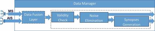
During the Validity Check we discard invalid messages, i.e. duplicate or contradicting positions and positions with invalid coordinates. Subsequently, the valid positions enter the Noise Elimination phase, where the goal is to identify and remove noisy positions. In more detail, we identify abnormal speeds and turns and positions which incur an abrupt change both in speed and heading of velocity. Finally, the noise-free stream is forwarded to the Synopses Generation phase, during which we discover the so-called “critical points,” which are points that indicate “instantaneous” (Pause, Change in Speed, Turn) and “long lasting” (Communication Gap, Long-term Stop, Slow Motion, Smooth Turn) events.

4.3. Mobility data enrichment

Mobility data is produced by vessel monitoring and identification systems or generated by algorithmic processes along the processing pipeline. The former case includes VMS and AIS data, while the latter case includes the products of data fusion and predictive analytics. Mobility Data in its basic form consists of records with a minimal set of fields, namely the vessel identifier, trace timestamp, and trace location in the form of geographical latitude and longitude, and optionally the speed, heading, and course of the vessel at the time. Basic Mobility Data lacks context that could be useful for better assessing the vessel’s state. Such context is the seabed depth at the location of the vessel, or the forecast for weather conditions at the vessel’s time and location. Mobility Data Enrichment is the process of augmenting basic mobility data with such additional contextual data, producing enriched mobility data suitable for further analysis. Both online and offline analyses benefit from working on enriched data, since costly processing operations, mainly spatio-temporal joins to geographical data, have already been applied. Filtering of mobility data based on these additional fields is much faster using enriched data, since the fields are readily available and no costly joins are required. This is especially beneficial to online filtering, which is applicable to the real-time presentation of the fleet state.

Basic mobility data is primarily extended with vessel attributes, geographical properties, and weather conditions for each reported time and location of the vessel. The vessel attributes used are the vessel type and length, which are obtained by joining to the vessel registry. The geographical properties used are the seabed depth, extracted from the bathymetry data spatial raster, and the marine area at the vessel’s location, obtained by spatially joining to the polygonal geometries representing marine areas defined by EU fishing regulations. The weather conditions included are wind speed and direction, wave height and direction, and rainfall intensity. The weather data is obtained by extracting the aforementioned values from the forecast or reanalysis meteorological data spatio-temporal raster. Forecast weather data, which can be supplied by a meteorological service, is used for the online enrichment of fresh mobility data with probabilistic future weather data. Reanalysis weather data, which is obtained from the European Center for Medium-Range Weather Forecasts (ECMWF) service (European Centre for Medium-Range Weather Forecasts Service), is used for the offline enrichment of historical mobility data with more accurate past weather data, yielding more refined historical mobility data. Enriched mobility data also include the activity indicator for fishing vessels. The activity indicator suggests whether a fishing vessel is most probably mooring, steaming, or fishing at the time. The activity indicator value is the result of a rule-based calculation that is provided by experts and takes into account the vessel type, the time of day and month of the trace timestamp, the vessel speed, and the distance of the vessel from the nearest port.

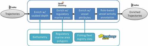
Mobility data enrichment is primarily implemented using Spark, wherein the availability of shared APIs for both offline and online processing has helped to reuse the enrichment methods developed for both analytics scenarios. For the determination of the marine area at the vessel’s location we employed the spatial join techniques provided by the (Apache Sedona Project). Those include spatial partitioning of both the mobility data and the marine area polygons so that spatial joins can be efficiently performed on each partition pair. For extracting values from raster datasets such as bathymetry and weather data, we used the (GeoTrellis Framework) to transform provided datasets to efficient layer structures stored in HDFS. The RasterFrames Library was used to handle these structures using Spark and join mobility data with time-dependent spatial rasters. Figure 6 illustrates how the various data enrichment steps can be combined in a stream processing pipeline using Kafka and Spark Streaming.

Figure 6. Mobility data enrichment streaming pipeline.

5. Offline analytics

5.1. Distributed Subtrajectory Join

An important operation, which is the cornerstone of several knowledge discovery techniques from mobility data, is the so-called trajectory join problem, which aims to find all pairs of “similar” (i.e. nearby in space-time) trajectories in a dataset. An even more challenging problem is the subtrajectory join query, where the goal is not only to identify all pairs of similar trajectories but also their corresponding “similar portions.” However, the subtrajectory join is a processing-intensive operation and centralized algorithms cannot scale with the size of today’s mobility data, thus parallel, and distributed algorithms are necessary in order to provide efficient processing of this query. As already mentioned, such a query is in fact the building block for several operations than aim to identify mobility patterns, such as co-movement patterns (Tritsarolis, Theodoropoulos, and Theodoridis 2020) and subtrajectory clustering (Pelekis et al. Pelekis, et al., 2017b; Tampakis et al. 2019). More specifically, within the scope of the i4sea platform, it can be utilized in order to identify illegal transshipment activity by retrieving all the pairs of moving objects that move “close” to each other for at least some duration, optimize transportation planning by merging “similar” itineraries or identify pairs of trajectories from different data sources (such as AIS and VMS) that represent the same moving objects. Motivated by these, we incorporate into the i4sea platform the Distributed Subtrajectory Join (DSJ) solution that was proposed in Tampakis et al. (2020).

In more detail, the problem that addresses is as follows: given two sets of trajectories, identify all pairs of maximal “portions” of trajectories (or else, subtrajectories) that move close in time and space w.r.t. a spatial threshold ${\epsilon }_{\mathit{sp}}$ and a temporal tolerance ${\epsilon }_t$, for at least some time duration $\mathit{\delta t}$. This can be depicted in Figure 7, given two trajectories $\mathit{r}$ and $\mathit{s}$, the pair of their maximal matching “portions” is ($\{r_4,r_5,r_6,r_7,r_8\},\{s_3,s_4,s_5,s_6,s_7\}$).

Figure 7. A pair of maximally “matching” subtrajectories $(r_{4,8},s_{3,7})$.

Formally, given a set $\mathit{R}$ of trajectories moving in the xy-plane, a trajectory $\mathit{r}\in \mathit{R}$ is a sequence of timestamped locations $\left\{r_1\dots r_N\right\}$. Each $r_i=(x_i,y_i,t_i)$ represents the $\mathit{i}$-th sampled point, $\mathit{i}\in 1,\dots \mathit{N}$ of trajectory $\mathit{r}$, where $\mathit{N}$ denotes the length of $\mathit{r}$ (i.e. the number of points it consists of). The pair $(x_i,y_i)$ and $t_i$ denote the 2D location in the xy-plane and the time coordinate of point $r_i$ respectively. A subtrajectory $r_{\mathit{i},\mathit{j}}$ is a subsequence $\left\{r_i\dots r_j\right\}$ of $\mathit{r}$ which represents the movement of the object between $t_i$ and $t_j$ where $\mathit{i}<\mathit{j}$.

Given a pair $(\mathit{r},\mathit{s})$ of trajectories (the same holds for subtrajectories) with $\mathit{r}\in \mathit{R}$ and $\mathit{s}\in \mathit{S}$, the common lifespan $w_{\mathit{r},\mathit{s}}$ is defined as the time interval $[\mathit{max}(r_1.\mathit{t},s_1.\mathit{t}),\mathit{min}(r_N.\mathit{t},s_M.\mathit{t})]$, where $r_1$ ($s_1$) is the first sample of $\mathit{r}$ ($\mathit{s}$, respectively) and $r_N$ ($s_M$) is the last sample of $\mathit{r}$ ($\mathit{s}$, respectively). The duration of the common lifespan $w_{\mathit{r},\mathit{s}}$ is $\mathrm{\Delta }{w}_{\mathit{r},\mathit{s}}$ = $\mathit{min}(r_N.\mathit{t},s_M.\mathit{t})$ – $\mathit{max}(r_1.\mathit{t},s_1.\mathit{t})$

Further, let $\mathit{DistS}(r_i,s_j)$ denote the spatial distance between two points $r_i$, $s_j$, which is defined as the Euclidean distance in this paper, even though other distance functions are also applicable. Also, let $\mathit{DistT}(r_i,s_j)$ denote the temporal distance, defined as $|r_i.\mathit{t}-s_j.\mathit{t}|$.

Definition 5.1. (Matching subtrajectories) Given a spatial threshold ${\epsilon }_{\mathit{sp}}$, a temporal tolerance ${\epsilon }_t$ and a time duration $\mathit{\delta t}$, a “match” between a pair of subtrajectories $(\mathit{r}{ }^{\mathrm{\prime }},\mathit{s}{ }^{\mathrm{\prime }})$ occurs iff $\mathrm{\Delta }{w}_{\mathit{r}{\mathit{ }}^{\mathrm{\prime }},\mathit{s}{ }^{\mathrm{\prime }}}\ge \mathit{\delta t}-2{\epsilon }_t$, and $\mathrm{\forall }\mathit{r}{{\mathit{ }}^{\mathrm{\prime }}}_{\mathit{i}}\in \mathit{r}{ }^{\mathrm{\prime }}$ there exists at least one $\mathit{s}{{\mathit{ }}^{\mathrm{\prime }}}_{\mathit{j}}\in \mathit{s}{ }^{\mathrm{\prime }}$ so that $\mathit{DistS}(\mathit{r}{{\mathit{ }}^{\mathrm{\prime }}}_{\mathit{i}},\mathit{s}{{\mathit{ }}^{\mathrm{\prime }}}_{\mathit{j}})\le {\epsilon }_{\mathit{sp}}$ and $\mathit{DistT}(\mathit{r}{{\mathit{ }}^{\mathrm{\prime }}}_{\mathit{i}},\mathit{s}{{\mathit{ }}^{\mathrm{\prime }}}_{\mathit{j}})\le {\epsilon }_t$, and $\mathrm{\forall }\mathit{s}{{\mathit{ }}^{\mathrm{\prime }}}_{\mathit{j}}$ there exists at least one $\mathit{r}{{\mathit{ }}^{\mathrm{\prime }}}_{\mathit{i}}$ so that $\mathit{DistS}(\mathit{s}{{\mathit{ }}^{\mathrm{\prime }}}_{\mathit{j}},\mathit{r}{{\mathit{ }}^{\mathrm{\prime }}}_{\mathit{i}})\le {\epsilon }_{\mathit{sp}}$ and $\mathit{DistT}(\mathit{s}{{\mathit{ }}^{\mathrm{\prime }}}_{\mathit{j}},\mathit{r}{{\mathit{ }}^{\mathrm{\prime }}}_{\mathit{i}})\le {\epsilon }_t$.

Definition 5.2. (Maximally matching subtrajectories) Given a pair of “matching” subtrajectories $(\mathit{r}{ }^{\mathrm{\prime }},\mathit{s}{ }^{\mathrm{\prime }})$ which belong to trajectories $\mathit{r},\mathit{s}$ respectively, this pair is considered a “maximal match” if $\text{setbox}0=\mathrm{\exists }\text{t}\mathit{o}\text{wd}0\text{hss}/\text{hss}\text{box}0$ superset $\mathit{r}{ }^{\mathrm{\prime \prime }}$ of $\mathit{r}{ }^{\mathrm{\prime }}$ or $\mathit{s}{ }^{\mathrm{\prime \prime }}$ of $\mathit{s}{ }^{\mathrm{\prime }}$ where the pair $(\mathit{r}{ }^{\mathrm{\prime \prime }},\mathit{s}{ }^{\mathrm{\prime }})$ or $(\mathit{r}{ }^{\mathrm{\prime }},\mathit{s}{ }^{\mathrm{\prime \prime }})$ or $(\mathit{r}{ }^{\mathrm{\prime \prime }},\mathit{s}{ }^{\mathrm{\prime \prime }})$ is “matching”.

At this point, we should clarify that two trajectories may have more than one “maximal matches” (i.e. pairs of subtrajectories). Having provided the above background definitions, we can define the subtrajectory join query between two sets of trajectories.

Definition 5.3. (Subtrajectory join) Given two sets of trajectories $\mathit{R}$ and $\mathit{S}$, a spatial threshold ${\epsilon }_{\mathit{sp}}$, a temporal tolerance ${\epsilon }_t$ and a time duration $\mathit{\delta t}$, the subtrajectory join query searches for all pairs $(\mathit{r}{ }^{\mathrm{\prime }},\mathit{s}{ }^{\mathrm{\prime }})$, $\mathit{r}{ }^{\mathrm{\prime }}\in \mathit{r}\in \mathit{R}$ and $\mathit{s}{ }^{\mathrm{\prime }}\in \mathit{s}\in \mathit{S}$, which are “maximally matching” subtrajectories.

To address this problem in a scalable manner, the MapReduce programming model was adopted. More specifically, the solution is comprised of a Repartitioning phase and a Query phase. The Repartitioning phase is a preprocessing step that takes place only once and the Query phase is where the actual processing takes place in a single MapReduce job. To boost the performance of the DSJ query processing even further, we introduce an indexing mechanism, which speeds up the computation of the . For more details about DSJ, please refer to (Tampakis et al. 2020).

5.2. Distributed Clustering

Another important operation that aims at discovering knowledge from mobility data is trajectory clustering. The research so far has focused mainly in methods that try to identify specific collective behavior patterns among moving objects (e.g. Tritsarolis, Theodoropoulos, and Theodoridis (2020)). However, these approaches operate at specific predefined temporal “snapshots” of the dataset, and by that they ignore the route of each moving object between these sampled points. Another line of research tries to identify patterns that are valid for the entire lifespan of the moving objects (e.g. T-OPTICS (Nanni and Pedreschi 2006)). Nevertheless, discovering clusters of complete trajectories can overlook significant patterns that might exist only for some portions of their lifespan.

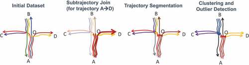
For this reason, we focus on Clustering analysis, where the goal is to segment trajectories to subtrajectories, according to some criteria, and then discover clusters of subtrajectories. In order to demonstrate the merits of subtrajectory clustering, let us consider the example of Figure 8, which illustrates six trajectories moving in the xy-plane, where each one of them has a different origin-destination pair. More specifically, these pairs are $\mathrm{A}\to \mathrm{B}$, $\mathrm{A}\to \mathrm{C}$, $\mathrm{A}\to \mathrm{D}$, $\mathrm{B}\to \mathrm{A}$, $\mathrm{B}\to \mathrm{C}$ and $\mathrm{B}\to \mathrm{D}$. These six trajectories have the same starting time and similar speed. A typical trajectory clustering technique would fail to identify any clusters. However, the goal of a subtrajectory clustering method is to identify four clusters ($\mathrm{A}\to \mathrm{O}$ (red), $\mathrm{B}\to \mathrm{O}$ (blue), $\mathrm{O}\to \mathrm{C}$ (purple), $\mathrm{O}\to \mathrm{D}$ (orange)) and two outliers ($\mathrm{O}\to \mathrm{A}$ and $\mathrm{O}\to \mathrm{B}$ (black)).

Figure 8. Clustering example of six trajectories moving in an intersection.

Within the i4sea platform, such an operation can be utilized in order to discover the underlying network of movement, which in the maritime domain this is apriori known, by grouping subtrajectories that move “close” to each other and use cluster representatives/medoids as network edges. An additional valuable application scenario of subtrajectory clustering is predictive analytics over mobility data, where the goal is the extraction of valuable knowledge from data and its utilization in order predict future behavioral patterns (i.e. movement) (Petrou et al. 2019, Petrou, et al., 2019). The general idea is first to identify popular mobility patterns, either global (for the whole dataset) or local (for each moving object separately), by employing some subtrajectory clustering technique that also provides the cluster representatives. Then, when some new position of a moving object is reported, the goal is to try to “match” the new portion of movement with the most similar historical patterns and employ this pattern in order to predict its future location.

To address this problem in the context of big data, we incorporate into the i4sea platform, the Distributed Subtrajectory Clustering (DSC) solution that was proposed in Tampakis et al. (2019). More specifically, DSC utilizes the MapReduce programming model by building upon the DSJ query (Tampakis et al. 2020), in order to tackle the problem in an efficient and scalable manner. In more detail, the problem of Subtrajectory Clustering is abstracted as a three-step procedure. The first step is the Subtrajectory Join, where for each trajectory $\mathit{r}$ we identify the maximal portions of all the other trajectory that moved “close enough” in time and space with $\mathit{r}$ (depicted in Figure 8). The next step is the Segmentation phase, where each trajectory gets segmented in subtrajectories whenever the density (or the composition) of its neighborhood changes “significantly.” Finally, we have the Clustering and Outlier Detection step, where the most “representative” subtrajectories get selected and the clusters get built “around” these “representatives.” For more details about the DSC solution, please refer to (Tampakis et al. 2019).

5.3. Hotspot Analysis

Hotspot Analysis is an important spatio-temporal operation that aims to detect statistically significant areas with high values, termed hotspots, as well as areas with low values, termed coldspots. Hotspot Analysis can be applied to a spatio-temporal feature dataset with regard to a specific feature value. The Getis-Ord $G_i^{\ast }$ statistic (Ord and Getis 1995), presented in Equation 1(1) $[\mathit{thb}]G_i^{\ast }=\frac{\sum _{\mathit{j}=1}^n{w}_{\mathit{i},\mathit{j}}{x}_j-\bar{x}\sum _{\mathit{j}=1}^n{w}_{\mathit{i},\mathit{j}}}{\mathit{s}\sqrt{\frac{\mathit{n}\sum _{\mathit{j}=1}^n{w}_{i,j}^2-{\left(\sum _{\mathit{j}=1}^n{w}_{\mathit{i},\mathit{j}}\right)}^2}{\mathit{n}-1}}}$(1) , is used for gauging the significance of each feature in the dataset. The $G_i^{\ast }$ statistic takes into account the spatio-temporal neighborhood of each feature. For a feature to be identified as a hotspot, the feature should generally have a high value and be among features with high values as well. Conversely, for a feature to be identified as a coldspot, the feature should generally have a low value and be among features with low values as well. The $G_i^{\ast }$ statistic smooths out features that stand out in their respective neighborhoods. The $G_i^{\ast }$ statistic is a z-score, interpreted as the number of standard deviations by which a raw score is above or below the raw score mean. In the i4sea platform, Hotspot Analysis operates on a set of spatio-temporal cells in the x, y, and t dimensions with respect to a cell value. The cells are the product of spatio-temporal segmentation. The range of each dimension and the cell size at each dimension are user-defined. The value of each cell is calculated before the $G_i^{\ast }$ statistic calculation. Requiring a confidence interval of 90%, cells with a $G_i^{\ast }$ statistic above 1.65 constitute the dataset hotspots, cells with a $G_i^{\ast }$ statistic below −1.65 constitute the dataset coldspots, and the rest of the cells are considered neutral. In more detail, the Getis-Ord $G_i^{\ast }$ statistic of feature $\mathit{i}$ can be defined as:

(1) $[\mathit{thb}]G_i^{\ast }=\frac{\sum _{\mathit{j}=1}^n{w}_{\mathit{i},\mathit{j}}{x}_j-\bar{x}\sum _{\mathit{j}=1}^n{w}_{\mathit{i},\mathit{j}}}{\mathit{s}\sqrt{\frac{\mathit{n}\sum _{\mathit{j}=1}^n{w}_{i,j}^2-{\left(\sum _{\mathit{j}=1}^n{w}_{\mathit{i},\mathit{j}}\right)}^2}{\mathit{n}-1}}}$(1)

where $\mathit{n}$ is the number of all features, $x_j$ is the value of feature $\mathit{j}$, and $w_{\mathit{i},\mathit{j}}$ is the weight of the neighborhood link between feature $\mathit{i}$ and feature $\mathit{j}$. The value of $w_{\mathit{i},\mathit{j}}$ is 1 if feature $\mathit{j}$ is in feature’s $\mathit{i}$ neighborhood, otherwise it is 0. $\bar{x}$ and $\mathit{s}$ are the usual mean and standard deviation of all feature values, respectively. Hotspot Analysis employs the Apache Spark framework. Spatio-temporal data points are initially mapped to and grouped by the spatio-temporal cells within which the data points fall and the cell values are accordingly calculated. The process is illustrated in Figure 9. The cell dataset is divided into multiple partitions according to the user parameters. A partition has the shape of a rectangular cuboid and consists of multiple cells at all dimensions. Each partition is assigned to a worker. With respect to a partition’s exterior cells, a part of a cell’s neighborhood is, by initial partition construction, assigned to neighboring partitions. Parallelism and performance are increased by making each cell along with its neighboring cells available to the same worker. The exact missing part of an exterior cell’s neighborhood depends on the neighborhood distance specified by the user and the position of the cell within the partition. In order to achieve data locality for these cells, parts of the exterior of the neighboring partitions must be transmitted to the worker processing the partition. The exact part of a partition’s exterior that needs to be transmitted to a neighboring partition depends on the relative positions of the two partitions and the neighborhood distance. An example of exterior cells from neighboring partitions that need to be transmitted to the worker processing a specific partition is illustrated in Figure 10. In this example, a neighborhood distance of 1 is assumed. After the repartitioning stage, all cells within a partition are colocated with their respective neighboring cells. The $G_i^{\ast }$ z-score is then calculated for each cell and the top-k, where k has been specified by the user, high score cells are returned to the Apache Spark application driver, concluding the analysis.

Figure 9. Data points are mapped to and grouped by cells, yielding a dataset of cells with a specific value.

Figure 10. Data locality in Hotspot Analysis. A worker is processing the partition with white cells. Gray cells denote exterior cells of neighboring partitions that are transmitted to the worker, so that the whole neighborhood of each white cell is made locally available to the worker.

An interesting application scenario of Hotspot Analysis, within the scope of the i4sea platform, is the estimation of fishing pressure, i.e. the intensity of fishing activity, is Fishing Pressure Hotspot Analysis. Fishing Pressure Hotspot Analysis aims to discover in which marine areas fishing activity is more intense and during which time periods, as well as marine areas of neutral and low fishing activity intensity. The activity indicator for a fishing vessel, namely the field that denotes which activity the vessel probably engages into at a specific time and location, is part of the enriched mobility data. Fishing Pressure Hotspot Analysis operates on the enriched mobility data for which fishing activity is indicated. Greek marine rules dictate fishing hours, which in turn make up fishing days, separately for each fishing vessel type. Trawlers and purse seiners, for instance, have different fishing hours. The marine rules are taken into consideration when temporally aggregating vessel traces of different vessel types. Fishing vessels with traces suggesting fishing activity are grouped by the containing spatio-temporal cells, yielding the aggregated fishing pressure value for each cell. Each vessel with at least one trace within a specific cell is counted exactly once, regardless of the number of traces, for the calculation of the cell value.

6. Online analytics

6.1. Co-Movement Pattern mining

Co-Movement Pattern mining (CMP) is yet another branch of Mobility Data Analytics, which focuses on discovering clusters of vessels that move together for at least some time duration. CMP can be employed in a wide plethora of applications, including traffic calculation and point-of-interest discovery, in different domains such as maritime, urban, and aviation.

In the context of the i4sea platform, the potential applications of Co-Movement Pattern mining are among many, anchorage discovery, naval surveillance for (probably suspicious) activities, such as transshipment and intentional AIS switch-off (Kontopoulos et al. 2020), as well as object and behavior profiling. Motivated by this, we adopt the approach of (Tritsarolis, Theodoropoulos, and Theodoridis 2020), where a novel graph-based online co-movement pattern mining algorithm is proposed, called EvolvingClusters, which can be used to discover different collective movement behaviors (e.g. flocks (Vieira, Bakalov, and Tsotras 2009), convoys (Jeung, Shen, and Zhou 2008; Jeung et al. 2008; Orakzai, Calders, and Pedersen 2019)) in a unified way based on the activity of multiple concurrent objects through time and space.

In a nutshell, given a Data stream $\mathit{D}=\{T_1,T_2,\dots ,T_n\}$ of Timeslices $T_i$ consisting of objects’ timestamped locations ($p_j$, $T_i$), EvolvingClusters works as follows:

• Each $p_j\in T_i$ is used in order to form a connectivity graph with vertices the points’ respective vessel identifier, and edges their spatial proximity with respect to a distance metric (e.g. Haversine distance) and a reachability threshold $\mathit{\theta }$

• Afterward, we extract the Maximal Connected Components (MCS $\approx$ Convoys) and Maximal Cliques (MC $\approx$ Flocks) with respect to a cardinality threshold $\mathit{c}$.

• Finally, each discovered pattern is compared to the previously discovered ones, and if it satisfies the temporal ($\mathit{t}$) and cardinality ($\mathit{c}$) restrictions, it is output to the resulted active patterns data stream.

The comparison between the members of two patterns $C_{t_i}$, $C_{t_i-1}$ discovered at timeslices $t_i$ and $t_{\mathit{i}-1}$, respectively, is conducted taking the following cases into account⁴:

1. The two patterns are identical ($C_{t_i}=C_{{\mathit{t}}_{\mathit{i}-1}}$)

2. The two patterns have no common objects ($C_{t_i}\cap C_{{\mathit{t}}_{\mathit{i}-1}}=\mathrm{\varnothing }$)

3. The current pattern is a subset of the previous one ($C_{t_i}\subset C_{{\mathit{t}}_{\mathit{i}-1}}$)

4. The current pattern is a superset of the previous one ($C_{{\mathit{t}}_{\mathit{i}-1}}\subset C_{t_i}$)

5. The two patterns contain only some common objects ($C_{t_i}\cap C_{{\mathit{t}}_{\mathit{i}-1}}\ne \mathrm{\varnothing }$, $C_{t_i}\cap C_{{\mathit{t}}_{\mathit{i}-1}}\subset C_{t_i},C_{{\mathit{t}}_{\mathit{i}-1}}$)

6.2. Predictive analytics

Predictive analytics over mobility data, is an important operation with a wide range of applications, such as collision detection, traffic estimation and service recommendation, in different domains, such as maritime, urban, and aviation. What is even more challenging is how to deal with this problem in the Big Data era, where new positions arrive at frequent rates and the accumulated ones scale to petabytes of data, and in application scenarios where latency and scalability matter.

There are several applications that could benefit from such an operation. For instance, in the maritime domain, detection and more importantly prevention of illegal fishing activity is of great impact in the preservation of marine life. More concretely, let us consider a scenario where a governmental agency tracks, in real time, the position of fishing vessels and its goal is not only to detect whether a fishing vessel has entered an area where fishing activities are forbidden but also to predict and prevent such kind of behavior by notifying the authorities.

In the maritime domain, the Future Location Prediction (FLP) of fishing vessels is of great importance, i.e. the prediction of the anticipated location(s) of a fishing vessel taking into account its own or the population’s motion history.

Definition 6.1. (FLP) Given a desired look-ahead interval $\mathrm{\Delta }{t}^{\mathit{pred}}$, the recent $\mathit{k}$ positions $r_{\mathit{N}-\mathit{k}+1},\dots ,r_N$ of moving object $\mathit{r}$, where, $r_N$ is the latest reported position, predict the position of $\mathit{r}$ at $t^{\mathit{now}}+\mathrm{\Delta }{t}^{\mathit{pred}}$, where $t^{\mathit{now}}$ is the current time.

6.2.1. LSTM-based FLP

Trajectories produced by vessels can be considered as time sequence data (Xue, Huynh, and Reynolds 2018) and thus are suited to be treated with techniques that are capable of handling sequential data and/or time series (Rossi et al. 2020). Several methods have been proposed to forecast time sequence data (Shi and Yeung 2018). However, over the past two decades, the research interest has been moved to Neural Networks (NNs) (Haykin 1998).

Long Short-Term Memory (LSTM) (Hochreiter and Schmidhuber 1997) is capable of learning long-term dependencies and has emerged as an effective NN architecture for several difficult learning problems (including sequential or temporal data-based applications) (Ji et al. 2020). Hence, in i4sea, we employ LSTMs to solve the future location prediction problem, that is, given vessel traffic data (timestamp, latitude, and longitude) and a time interval $\mathrm{\Delta }{t}^{\mathit{pred}}$, to predict each vessel’s location after $\mathrm{\Delta }{t}^{\mathit{pred}}$ time. Details for the LSTM NNs can be found in the original publications (Graves and Schmidhuber 2005).

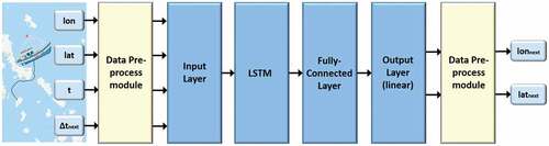
A schematic overview of the proposed LSTM-based network architecture is presented in Figure 11. More specifically, the NN architecture is composed of a data pre-process module, which transforms appropriately the AIS data to feed LSTM model, an input layer of four neurons (one for each input variable), an LSTM hidden layer, a fully connected hidden layer, an output layer of two neurons (one for each prediction coordinate) and a data pre-process module to transform appropriately the NN outputs to the predicted latitude and longitude coordinates. Details for the Backward Propagation Through Time algorithm and for the Adam approach, which were employed for the NN learning purposes, can be found in Werbos (1990) and Kingma and Ba (2015), respectively.

Figure 11. Network architecture for the proposed LSTM model, with one LSTM cell and two fully connected layers. The dark blue boxes indicate layers in the network, while the light blue ones indicate the input-output information.

6.2.2. Activity prediction

The operation of activity prediction, in the context of the i4sea platform, is, given a lookahead interval $\mathrm{\Delta }{t}^{\mathit{pred}}$, to predict whether a fishing vessel will be fishing at $t^{\mathit{now}}+\mathrm{\Delta }{t}^{\mathit{pred}}$. The way that this operation is actually implemented in the i4sea platform brings up the merits of the i4sea architecture, since different modules are combined into a pipeline. More specifically, as illustrated in Figure 12, the Trajectory Prediction (TP) and the Mobility Data Enrichment modules are utilized. In more detail, the TP module predicts the route of each moving object from $(t^{\mathit{now}},t^{\mathit{now}}+\mathrm{\Delta }{t}^{\mathit{pred}}]$, and these prediction are given as input to the Mobility Data Enrichment module which applies the rule-based activity annotation. The output, will be a new stream that will contain the information about the activity that each fishing vessel will be performing at $t^{\mathit{now}}+\mathrm{\Delta }{t}^{\mathit{pred}}$. In a similar direction the Future Location Prediction and the Co-Movement Pattern mining module where utilized in order to predict future patterns of movement, as presented in (Tritsarolis et al. 2021).

Figure 12. Activity prediction pipeline.

7. Application Layer

7.1. Monitoring

Presenting and monitoring online analytics results is particularly challenging, especially in the case of geospatial data such as trajectories, that span both space and time dimensions. The Application Layer defines building blocks for such applications that leverage Web Service principles in order to expose analysis results to the web, so that they can be visualized in web applications. This way, access to the platform cluster can be provided with minimal exposure of cluster nodes to the outside of the cluster private network.

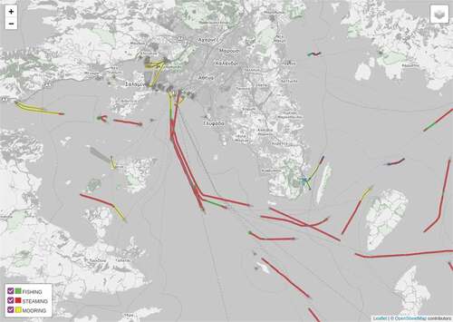
Figure 13 illustrates the architecture of an application prototype targeted to online analytics results monitoring. The application aims to monitor the evolving state of the entire fishing fleet, with regard to the last known position of each vessel. Input mobility data messages of trajectories are sent to a Kafka topic. Input mobility data must conform to a general trajectory schema where at least the location, timestamp, and vessel identifier are provided by the message source. The streams processing pipeline operates on input mobility data and produces output mobility data, specifically enriched trajectories, trajectory synopses, enriched trajectory synopses, trajectory predictions, and enriched trajectory predictions. The output mobility data produced is forwarded to the respective Kafka topics. Input and output mobility data is periodically written by a Python application to a SQLite database, which constitutes the fleet state database. A Flask-based Web Service is deployed within the platform cluster network and acts as a gateway to the analytics results for the outside world. A Web Application running on a Web Browser polls the service for the most recent fleet state data. The service queries the SQLite database to retrieve fleet state data according to user-specified query criteria. The data retrieved is then transferred to the Web Browser using JSON representation and presented on a map using visualization methods provided by the Leaflet web map library. A map view of the online analytics results monitoring application prototype, which displays fishing vessel activity, is presented in Figure 14.

Figure 13. Application prototype for online analytics results monitoring.

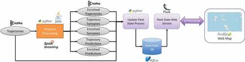
Figure 14. Fishing vessel activity view of the online analytics results monitoring application prototype. A fishing vessel is depicted as either mooring, steaming, or fishing.

8. Experimental evaluation

The experiments were conducted in a 9-node cluster, running Hortonworks Data Platform version 3.1.0.0, where each node has 16GB of memory and 8-core CPUs. The storage subsystem is implemented as part of the cluster using HDFS, providing a total of 3.3 TB distributed in 7 nodes. Spark execution engine is deployed across 7 nodes also, using Apache Hadoop YARN as the resource manager.

For our experimental study, we utilize 2 years (2017 and 2018) of AIS and VMS data of fishing vessels moving in Greek waters. The vessel movement data include anonymized VMS data provided by the Administration of Fishery Control, Ministry of Maritime and Insular Policy of Greece. They include about 50 million position reports from more than 1000 fishing vessels and take up about 2GB of storage space in compressed form (gzip). We also used a more extensive dataset of terrestrial AIS data, sourced by the Administration of Maritime Safety, Minister of Maritime Affairs and Insular Policy of Greece. The AIS dataset includes about 3.7 billion position reports from more than 10,000 vessels, taking up more than 60GB in storage space compressed (gzip). We also utilized meteorological re-analyis data available via the European Center for Medium-Range Weather Forecasts (ECMWF) data portal, covering the sea area of Greece and spanning the same two-year period. They include hourly values for 11 significant measures related to weather conditions at sea. Additional data used primarily for data enrichment also include a bathymetry spatial raster dataset from EMODnet, as well as polygonal geometries representing marine areas defined by EU fishing regulations, processed and contributed to the project by the Hellenic Center for Marine Research (HCMR), partner to the i4sea project.

Our experimental methodology is as follows. Initially, we evaluate the Data Fusion component in term of quality of results. Subsequently, we examine the efficiency and the effectiveness of the Synopses Generator, in terms of latency and compression rate. Next, we examine the efficiency of the Mobility Data Enrichment process in both noise-free raw data and the corresponding synopses. Successively, we evaluate the quality of the Distributed Subtrajectory Clustering component by comparing with two state-of-the-art subtrajectory clustering algorithms. Furthermore, we present a demonstration of the Hotspot Analysis and the Co-movement Pattern Mining components. Finally, we evaluate the efficiency and the effectiveness of the Future Location Prediction component.

8.1. Data preparation

8.1.1. Data Fusion

For the evaluation of the Data Fusion component, we utilized a subset of the VMS and AIS datasets corresponding to the same period, i.e. January 2018. The reason for choosing a subset of 1 month duration is that we needed to manually extract the ground truth for the experiment that follows, which made it impossible to use the entire dataset. Concerning the efficiency and scalability of the DMSTJ solution, please refer to (Tampakis et al. 2020). The VMS dataset contained 637 fishing vessels and the corresponding AIS dataset contained 1045 fishing vessels. At this point, we should mention that, by law, not all fishing vessels are obliged to carry a VMS device, only those that exceed a specific length. Furthermore, not all fishing vessels carry an AIS device, which means that the number of vessels that hold both an AIS and a VMS device might be relatively small in comparison with the total number of fishing vessels that hold either an AIS or a VMS device. Moreover, concerning the fishing vessels that carry an AIS device, only the ones that exceed a specific length are obliged by law to transmit their position at all times.

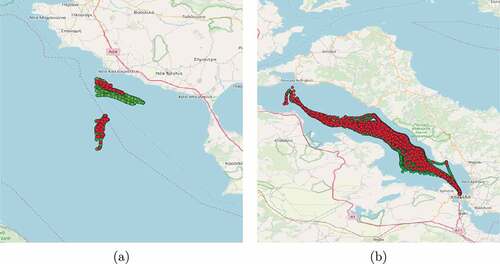
In practice, we ran DMSTJ, with the following parameter setting, ${\epsilon }_{\mathit{sp}}=10\mathrm{km}$, ${\epsilon }_t=10\min$, $\mathit{\delta t}=20\min$ and $\mathit{\alpha }=0.2$ and we managed to achieve 52 “matches.” However, evaluating a solution where the ground truth is unknown is a difficult task. For this reason, we utilized two alternative methods in order to achieve this, visual inspection and manual ground truth based on the names and the other contextual information of the vessels. In terms of visual inspection, the results are satisfying since it seems, as illustrated in Figure 15, that the vast majority of the discovered matches correspond to the same fishing vessel. Concerning the manual ground truth, as illustrated in Table 1, there were 210 fishing vessels that appeared in both datasets by examining the name and other contextual information. This leads to accuracy and precision at approximately 0.84, as depicted in Table 1. Moreover, by visually inspecting the cases that were falsely identified as “matches,” at least half of them seemed to belong to the same vessel. All in all, it seems that our solution manages to identify a large number of AIS/VMS “matches,” given the fact that the number of fishing vessels that hold both an AIS and a VMS device is relatively small and the fact that a large number of fishing vessels, that carry an AIS device, are obliged by law to transmit their position at all times.

Table 1. AIS/VMS fusion confusion matrix with accuracy and precision

	Discovered				Accuracy	Precision
Actual		True	False	Total	0.833493	0.846154
	Positive	44	166	210
	Negative	8	827	835
	Total	52	993	1045

Figure 15. Examples of discovered matches between VMS (red) and AIS (green).

8.1.2. Synopses Generation

Initially, we evaluate the effectiveness of the synopses generator as a tool to reduce the amount of data by keeping only the critical points. We ran the Synopses Generator in 2 years of AIS data (i.e. 2017–2018) and calculated the compression rate. As illustrated in Table 2, the initial noise-free number of positions in the dataset was approximately 100 million, while the number of critical points that were extracted was about 11 million, which results in a compression rate of 88.37%.

Table 2. Compression rate of Synopses Generator

Number of Positions	Critical Points	Compression Rate
101281869	11778948	88.37%

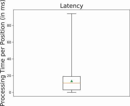
Subsequently, we evaluate the efficiency of the synopses generation procedure, by means of processing time per position. As illustrated in Figure 16, the Synopses Generator conforms with the real-time nature of the i4sea platform, since the media processing time of a position is 11 milliseconds.

Figure 16. Performance of the Synopses Generator in terms of latency.

8.1.3. Mobility data enrichment

For the experimental evaluation of online mobility data enrichment, we used two datasets of AIS data. The first AIS dataset consists of noise-free AIS data. The total number of traces in the dataset is depicted in Table 2. The second AIS dataset consists of AIS synopses data produced by the first dataset. The total number of traces is also depicted in Table 2. The experiments were run on Apache Spark Streaming with four different setups. More specifically, we experimented with the trigger interval option set to 1, 2, 4 and 8 minutes, which means that whenever a batch of data with durations 1, 2, 4 and 8 minutes gets accumulated, the mobility data enrichment process gets triggered for the specific batch. For each setup, we measured the median time needed by Apache Spark Streaming to process the input batches and produce the enriched mobility data. The results of the experiment are presented in Table 3.

Table 3. Experimental evaluation of online mobility data enrichment in Apache Spark Streaming. Noise-free AIS traces vs AIS Synopses processed using trigger interval option set to 1, 2, 4 and 8 minutes

	Median Latency (in msec)
Trigger Interval	Noise-Free Raw Data	Synopses
1	31.54	2.87
2	60.33	5.35
4	115.67	10.32
8	226.21	20.67

As it is obvious, the processing time of the synopses is about an order of magnitude faster than processing the noise-free raw dataset. As anticipated this result is aligned with the compression rate, i.e the critical points is about 11% of the noise-free raw dataset and the processing time of the critical points is about 11% of the processing time of the noise-free raw dataset.

8.2. Offline analytics

8.2.1. Distributed Subtrajectory Clustering

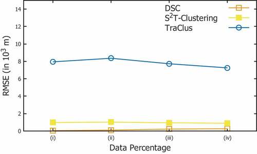
We compare DSC with two state-of-the-art subtrajectory clustering algorithms, S²T-Clustering (Pelekis et al. Pelekis, et al., 2017b) and TraClus (Lee, Han, and Whang 2007). The metric that we employ in order to evaluate the quality of the outcome of the clustering procedure is the well-known RMSE metric, which is actually a measure of intra-cluster distance between the representatives and the cluster members. Hence, the larger the RMSE, the higher the intra-cluster distance and consequently the lower the quality of the clustering.

In order to perform this experiment, we utilized a month of noise-free data from July 2018 which was further partitioned in 4 portions (25%, 50%, 75%, 100%). This choice was necessary because the centralized implementations of S²T-Clustering and TraClus could not scale with the full size of the datasets. As illustrated in Figure 17, DSC outperforms, in terms of RMSE, both TraClus and S²T-Clustering.

Figure 17. Comparison between DSC, S²T-Clustering and TraClus in terms of the RMSE metric.

8.2.2. Hotspot Analysis

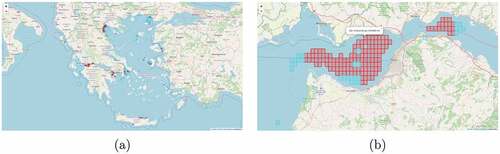
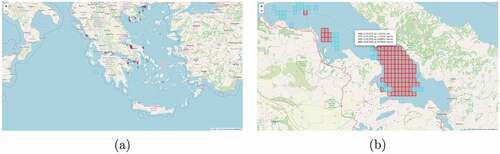
A demonstration of Hotspot Analysis applied to AIS data is presented in Figure 18. The analysis parameters consist of trawler for the vessel type, fishing for the vessel activity, a bounding box of Greece for the spatial range, and January 2018 for the temporal range. The cell dimensions are 0.015 degrees at the longitude dimension, 0.015 degrees at the latitude dimension, and the whole temporal range at the temporal dimension. The neighborhood distance is set to 2. This makes sense for the longitude and latitude dimensions. Since there is a single timespan at the temporal dimension, each cell has no neighboring cells at this dimension. The top-2000 cells are displayed. Hotspots are displayed as red rectangles, coldspots as deep blue rectangles, and neutral cells as light blue rectangles. Since hotspots are exhausted before the 2000-limit is reached, several neutral cells are displayed as well as all the hotspots. Only cells with at least one vessel fishing within the cell are displayed.

Figure 18. Fishing Pressure Hotspot Analysis of trawler AIS data. The data spans one month from 1 January 2018 to 31 January 2018 and is temporally grouped by the whole temporal range. The figure displays (a) the overview and (b) a detail of the analysis result.

A popup at each rectangle’s location displays the rank, timespan start date, and $G_i^{\ast }$ statistic of the underlying cell. It also indicates whether the cell is a hotspot, is neutral, or is a coldspot.

A demonstration of Hotspot Analysis applied to AIS and VMS data is presented in Figure 19. The analysis parameters consist of 50 m for the minimum depth at the trace location, purse seiner for the vessel type, fishing for the vessel activity, a bounding box of Greece for the spatial range, and January to August 2018 for the temporal range. The cell dimensions are 0.015 degrees at the longitude dimension, 0.015 degrees at the latitude dimension, and 15 days at the temporal dimension. The neighborhood distance is set to 2. The top-3000 cells are displayed. Since hotspots are exhausted before the 3000-limit is reached, several neutral cells are displayed as well as all the hotspots.

Figure 19. Fishing Pressure Hotspot Analysis of purse seiner AIS and VMS data at depths greater than 50 m. The data spans eight months from 1 January 2018 to 31 August 2018 and is temporally grouped by 15-day timespans. The figure displays (a) the overview and (b) a detail of the analysis result.

A popup at each rectangle’s location displays the rank, timespan start date, and $G_i^{\ast }$ statistic of the underlying cell or cells. It also indicates whether each cell is a hotspot, is neutral, or is a coldspot. Each rectangle may correspond to a single cell or multiple cells, since there are multiple timespans at the temporal dimension, and is colored according to the highest ranking cell underneath. The cells within the popup are listed in descending ranking order.

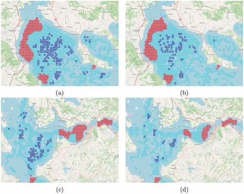
A demonstration of Hotspot Analysis applied to AIS complete data in contrast to AIS synopses data is presented in Figure 20. The analysis parameters are identical in both cases and consist of trawler for the vessel type, fishing for the vessel activity, a bounding box of Greece for the spatial range, and January to March 2018 for the temporal range. The cell dimensions are 0.015 degrees at the longitude dimension, 0.015 degrees at the latitude dimension, and 15 days at the temporal dimension. The neighborhood distance is set to 2. All cells with at least one vessel fishing within the cell are displayed.

Figure 20. Fishing Pressure Hotspot Analysis of trawler AIS complete data in contrast to AIS synopses data. The data spans three months from 1 January 2018 to 31 March 2018 and is temporally grouped by 15-day timespans. The figure displays two details of the analysis result for the AIS complete data in (a) and (c) and the corresponding details of the analysis result for the AIS synopses data in (b) and (d). AIS synopses data, although much sparser than AIS complete data, seems to perform well enough in this case, successfully identifying the vast majority of hotspots.

8.3. Online analytics

8.3.1. Co-Movement Pattern mining

Focusing on the maritime domain, Figure 21 illustrates the EvolvingClusters formed at 1 August 1 2018 within 00:00–05:00. More specifically, we observe that most patterns are formed at nearby ports, with some of them being either anchorages or fishing ports. Focusing on the Saronic Gulf, where most traffic is located, we observe in addition some potential fishing areas near the Islands Salamina and Aegina.

Figure 21. Toward the exploitation of EvolvingClusters in Maritime Domain (left: MCS; right: MC). Discovering anchorages and (potential) fishing areas.

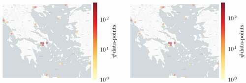
In conclusion, running EvolvingClusters within the entirety of the dataset’s temporal horizon may uncover several other patterns, indicating the presence of (probably suspicious) phenomena such as over-fishing (i.e. fishing pressure level) or transshipment and intentional AIS switch-off (Kontopoulos et al. 2020). These findings may inspire domain experts into further investigating these occurrences and reach some meaningful deductions.

8.3.2. LSTM-based FLP

NNs require massive amounts of data for learning purposes. In the literature, the employed datasets for vessel FLP purposes using NN models, often, include records obtained from vessels during one-month period (Tu et al. 2018; Valsamis et al. 2017). Particularly, in Tu et al. (2018), the selected dataset contained 403,599 AIS records from 180 vessels of different types. In this paper, in order to employ sufficient data for vessel FLP purposes, the proposed NN model was experimentally evaluated over a sample dataset of 1,078,544 AIS records received from 507 fishing vessels, during the whole year of 2018, in the Aegean Sea rectangle bounded by latitude in [36.0846 … 39.4871] and longitude in [24.4556 … 26.5869].

For each vessel, original AIS sequences are being partitioned into a number of meaningful trajectories, then a method evaluation procedure, similar to (Alexandridis et al. 2017) was adopted, i.e. the available trajectories were allocated randomly into three sets: training, validation and testing, employing 50%–25%–25% ratio, respectively. Obviously, the three sets include different trajectories of the available vessels, i.e. data of the training set cannot be found in the validation or testing sets. Also, in order to prevent even the slightest chance of data leak, special care was taken for trajectories of the same vessel occurring on the same day not to be allocated into different sets.

Moreover, the NN parameters were determined using the training set and then model selection was performed using the validation set. Finally, the selected NN model’s performance was tested on the testing set, which is independent of training and model selection and thus can assess generalization capabilities.

As far as the testing phase is concerned, by taking advantage of the i4sea architecture, the vessels’ next position prediction corresponds to an online distributed procedure. More specifically, streaming information from different vessels is fed to the network at the same time, which a) makes predictions in parallel and b) sends the new information in a distributed streaming way to other tools in the i4sea platform.

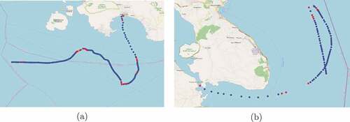
Experimental results were evaluated using the Mean Absolute Error (MAE) of the Euclidean distance between the original points and the predicted ones on the testing set. According to the results, the LSTM model predicts satisfactorily the fishing vessels’ next position. More specifically, for the prediction intervals 2, 5, 10, 20, and 30 minutes, the respective MAE, in the testing set, are 50, 128, 337, 753, and 1714 meters. For visualization purposes Figure 22(a) shows a fishing vessel’s original locations along with the predicted ones, for each prediction interval.

Figure 22. (a) Original locations vs Predicted locations for a fishing vessel and (b) Performance of the FLP tool in terms of latency.

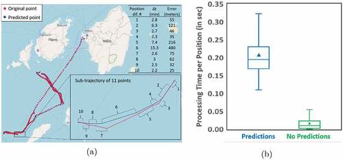
Figure 22(b), also, depicts time-related efficiency of the LSTM-based FLP on the i4sea platform, by means of processing time per predicted position and non prediction, i.e. non processed data.

9. Conclusions – future work

To conclude, in this paper we present the i4sea Big Data platform, which aims at monitoring and analyzing the activity of fishing vessels by following a lambda architecture that facilitates access to both batch processing and stream processing methods with a hybrid approach and thus balancing between latency, throughput, and fault tolerance. Moreover, we presented several characteristic use-case scenarios, such as Mobility Data Enrichment, AIS/VMS Fusion, Distributed Subtrajectory Join and Clustering, Hot-spot Analysis, Co-movement Pattern Discovery and Vessel Future Location Prediction, which are seamlessly integrated into the i4sea platform by utilizing the publish-subscribe communication system (Kafka).

As for future work, we plan to integrate additional data sources, such as ERS (electronic reporting system), which are daily electronic logs of fishing vessels that refer to the quantities of catches and RTH, which are real-time data from radars and thermal cameras. Moreover, we plan to extend the functionality of the i4sea platform, so that it will be able to support additional use case scenarios by creating new pipelines of the already existing functionality and by seamlessly integrating novel offline and online analytics. Finally, we would like to investigate whether the existing architecture of the i4sea platform can be used in other domains, such as sustainable fishing tourism.

Data availability statement

The AIS and VMS datasets used in our experimental study cannot be made publicly available due to national legislative constraints. However, a subset of the AIS dataset which was collected by our AIS antenna can be found at https://doi.org/10.5281/zenodo.4498410.

Disclosure statement

No potential conflict of interest was reported by the authors.

Additional information

Funding

This work was partially supported by the Greek Ministry of Development and Investment, General Secretariat of Research and Technology, under the Operational Programme Competitiveness, Entrepreneurship and Innovation 2014–2020 [grant T1EDK-03268, i4sea].

Notes on contributors

Panagiotis Tampakis

Panagiotis Tampakis received the PhD degree in Big Mobility Data Management and Analytics from the Department of Informatics of University of Piraeus. He is currently an Assistant Professor at the Department of Mathematics and Computer Science of the University of Southern Denmark. His has an exceptional publication record in top venues and journals and has participated in several EU-funded research projects. His research interests include mobility data management and mining and big data.

Eva Chondrodima

Eva Chondrodima received the Ph.D. degree in computational intelligence from the National Technical University of Athens (NTUA), Greece, in 2017, the M.Sc. degree in advanced information systems from the University of Piraeus, Greece, in 2013, and the B.Sc. degree in electronic engineering from the Technological Educational Institute of Athens, Greece, in 2011. She is currently a Post-Doctoral researcher with the Department of Informatics, University of Piraeus. Her research interests include computational intelligence with emphasis on neural networks and evolutionary computation methods, and applications to geoscience, mobility data science, and semantic Web.

Andreas Tritsarolis

Andreas Tritsarolis holds a BSc in Informatics (University of Piraeus, 2020) and currently studies Data Science and Machine Learning at MSc level. He also participates as a junior researcher at the Data Science Lab, University of Piraeus, collaborating in a number of research projects. His research interests lie in the areas of Data Science and Machine Learning for Mobility Data, with emphasis on Deep and Federated Learning. He has co-authored papers in refereed journals (including IJGIS) and conference proceedings (including MDM and SSTD), in the field of Mobility Data Analytics.

Aggelos Pikrakis

Aggelos Pikrakis (Eng. ‘93, Ph.D. ‘02) is an Assistant Professor (tenured position) at the Department of Informatics, University of Piraeus, Greece, teaching courses related to Machine Learning, Digital Signal Processing and Audio Analysis. His research interests lie primarily in the area of audio analytics, with an emphasis on machine learning algorithms, including deep neural networks, Hidden Markov models, Bayesian architectures and alignment methods. He is the co-author of two internationally acclaimed textbooks and more than 50 refereed articles in peer-reviewed journals and conferences, with his research work ranking high in various international algorithmic challenges. He is also the recipient of the 2019 EURASIP Meritorious Service Award. For more information, please see Aggelos’s homepage at http://www.cs.unipi.gr/pikrakis, his Google Scholar page and his GitHub page at https://github.com/pikrakis

Yannis Theodoridis

Yannis Theodoridis is Professor of Data Science at the University of Piraeus, Greece. His research interests include big data management & analytics for human mobility- related information. He has co-authored three monographs and over 100 refereed articles in scientific journals and conferences, with over 12,000 citations so far, according to Google Scholar. He holds a Dipl. Eng. (1990) and Ph.D. (1996) in Computer Engineering, both from the National Technical University of Athens (NTUA). Personal webpage: http://www.unipi.gr/faculty/ytheod/.

Kostis Pristouris

Kostis Pristouris is an experienced software engineer with a diploma in electrical & computer engineering and a postgraduate diploma in geoinformatics, both from the National Technical University of Athens. He is a full stack engineer, with strong experience in web development and databases, particularly versed in geographic information systems applications and infrastructure.

Harry Nakos

Harry Nakos is an electrical and computer engineer from the National Technical University of Athens. He works as a scientific associate at the Athena Research Center in Athens. His professional and research interests include web application development, geospatial data analysis, and social network data analysis.

Panagiotis Kalampokis

Panagiotis Kalampokis received his Bsc diploma in Computer Science from University of Ioannina Greece in 2013, and his Msc in Mobile and Web Development from International Hellenic University in 2017 with main focus on Big Data Analytics. Since 2018 he has been working as a Big Data Developer in many R&D projects e.g: (SLIPO, I4Sea) at IMSI Institute of Athena Research and Innovation Center. His current research interests include GeoSpatial Analysis with Big Data and Web Development.

Theodore Dalamagas

Theodore Dalamagas is Research Director, Vice Director of Information Management Systems Institute at ATHENA Research Center, co-founder and Chief Technology Officer of Symbiolabs (spinoff of ATHENA). He received his Diploma in Electrical Engineering from NTU Athens, Greece, his MSc in Advanced Information Systems from Glasgow University, Scotland, and his PhD from NTUA. His research and technology areas of interest include: scientific databanks and e-research infrastructures, data Web and information retrieval, data interoperability and integration, and bioinformatics.

Notes

1. Sea Observer (COSMOS), Fishery Solution: vTrack Vessel Monitoring (Visma Consulting A/S) and Trackwell VMS (Trackwell Ltd.)

2. http://cosmosconsulting.gr/wp-content/uploads/pdf/SeaObserverVMS.pdf.

3. The source code can be found here: https://github.com/DataStories-UniPi/Distributed-Subtrajectory-Similarity-Matrix.

4. For more information regarding the above discussion the reader is referred to (Tritsarolis, Theodoropoulos, and Theodoridis 2020).

References

- Alexandridis, A., E. Chondrodima, N. Giannopoulos, and H. Sarimveis. 2017. “A Fast and Efficient Method for Training Categorical Radial Basis Function Networks.” IEEE Transactions on Neural Networks and Learning Systems 28 (11): 2831–2836. doi:10.1109/TNNLS.2016.2598722.
- AMINESS Project. http://aminess.eu
- Anagnostopoulos, T., C. Anagnostopoulos, and S. Hadjiefthymiades. 2011. “Mobility Prediction Based on Machine Learning.” In 12th IEEE International Conference on Mobile Data Management, MDM 2011, Luleå, Sweden, June 6–9, 2, 27–30.
- Apache Sedona Project. https://sedona.apache.org
- Armbrust, M., T. Das, J. Torres, B. Yavuz, S. Zhu, R. Xin, A. Ghodsi, I. Stoica, and M. Zaharia. 2018. “Structured Streaming: A Declarative API for Real-time Applications in Apache Spark.” In Proceedings of the 2018 International Conference on Management of Data, SIGMOD Conference 2018 Houston, TX, USA, edited by G. Das, C. M. Jermaine, and P. A. Bernstein, 601–613. ACM.
- Bakalov, P., M. Hadjieleftheriou, E. J. Keogh, and V. J. Tsotras. 2005. “Efficient Trajectory Joins Using Symbolic Representations.” In Proceedings of MDM Ayia Napa, Cyprus, 86–93.
- BlueBRIDGE project. http://www.bluebridge-vres.eu
- Chen, Y., and J. M. Patel. 2009. “Design and Evaluation of Trajectory Join Algorithms.” In Proceedings of SIGSPATIAL Seattle, Washington, USA, 266–275.
- DatAcron project. http://ai-group.ds.unipi.gr/datacron
- European Centre for Medium-Range Weather Forecasts service. https://www.ecmwf.int
- Fang, Y., R. Cheng, W. Tang, S. Maniu, and X. S. Yang. 2016. “Scalable Algorithms for Nearest-neighbor Joins on Big Trajectory Data.” IEEE Transactions on Knowledge and Data Engineering 28 (3): 785–800. doi:10.1109/TKDE.2015.2492561.
- FERARI project. http://www.ferari-project.eu
- GeoTrellis framework. https://geotrellis.io
- Gormley, C., and Z. Tong. 2015. Elasticsearch: The Definitive Guide: A Distributed Real-time Search and Analytics Engine. Sebastopol, California: O’Reilly Media.
- Graves, A., and J. Schmidhuber. 2005. “Framewise Phoneme Classification with Bidirectional Lstm and Other Neural Network Architectures.” Neural Networks 18 (5): 602–610. IJCNN 2005. doi:10.1016/j.neunet.2005.06.042.
- Haykin, S. 1998. Neural Networks: A Comprehensive Foundation. 2nd ed. USA: Prentice Hall PTR.
- Hochreiter, S., and J. Schmidhuber. 1997. “Long Short-term Memory.” Neural Computation 9 (8): 1735–1780. doi:10.1162/neco.1997.9.8.1735.
- Hong, L., Y. Zheng, D. Yung, J. Shang, and L. Zou. 2015. “Detecting Urban Black Holes Based on Human Mobility Data.” In Proceedings of SIGSPATIAL Bellevue, WA, USA.
- i4sea project. https://i4sea.eu
- INFORE project. http://www.infore-project.eu
- Jeung, H., H. T. Shen, and X. Zhou. 2008. “Convoy Queries in Spatio-temporal Databases.” In ICDE Auckland, New Zealand, 1457–1459. IEEE Computer Society.
- Jeung, H., M. L. Yiu, X. Zhou, C. S. Jensen, and H. T. Shen. 2008. “Discovery of Convoys in Trajectory Databases.” PVLDB 1 (1): 1068–1080.
- Ji, Y., L. Wang, W. Wu, H. Shao, and Y. Feng. 2020. “A Method for Lstm-based Trajectory Modeling and Abnormal Trajectory Detection.” IEEE Access 8: 104063–104073. doi:10.1109/ACCESS.2020.2997967.
- Kalnis, P., N. Mamoulis, and S. Bakiras. 2005. “On Discovering Moving Clusters in Spatio-temporal Data.” In SSTD Angra dos Reis, Brazil, 364–381.
- Kingma, P. D., and J. Ba. 2015. “Adam: A Method for Stochastic Optimization.” In International Conference on Learning Representations (ICLR) San Diego, CA, USA.
- Kontopoulos, I., K. Chatzikokolakis, D. Zissis, K. Tserpes, and G. Spiliopoulos. 2020. “Real-time Maritime Anomaly Detection: Detecting Intentional AIS Switch-off.” International Journal of Big Data Intelligence 7 (2): 85–96. doi:10.1504/IJBDI.2020.107375.
- Kreps, J., N. Narkhede, and J. Rao. 2011. “A Distributed Messaging System for Log Processing.” In Proceedings of 6th International Workshop on Networking Meets Databases (NetDB), Athens, Greece.
- Laube, P., S. Imfeld, and R. Weibel. 2005. “Discovering Relative Motion Patterns in Groups of Moving Point Objects.” IJGIS 19 (6): 639–668.
- Lee, J., J. Han, and K. Whang. 2007. “Trajectory Clustering: A Partition-and-group Framework.” In SIGMOD Beijing, China, 593–604.
- Li, Y., J. Bailey, and L. Kulik. 2015. “Efficient Mining of Platoon Patterns in Trajectory Databases.” Data & Knowledge Engineering 100: 167–187. doi:10.1016/j.datak.2015.02.001.
- Li, Z., B. Ding, J. Han, and R. Kays. 2010. “Swarm: Mining Relaxed Temporal Moving Object Clusters.” PVLDB 3 (1): 723–734.
- Lukasczyk, J., R. Maciejewski, C. Garth, and H. Hagen. 2015. “Understanding Hotspots: A Topological Visual Analytics Approach.” In Proceedings of SIGSPATIAL Bellevue, WA, USA.
- Makrai, G. 2016. “Efficient Method for Large-scale Spatio-temporal Hotspot Analysis.” In Proceedings of SIGSPATIAL California, USA.
- Moran, P. 1950. “Notes on Continuous Stochastic Phenomena.” Biometrika 37 (1): 17–23. doi:10.1093/biomet/37.1-2.17.
- Nanni, M., and D. Pedreschi. 2006. “Time-focused Clustering of Trajectories of Moving Objects.” Journal of Intelligent Information Systems 27 (3): 267–289. doi:10.1007/s10844-006-9953-7.
- Nikitopoulos, P., A. Paraskevopoulos, C. Doulkeridis, N. Pelekis, and Y. Theodoridis. 2018. “Hot Spot Analysis over Big Trajectory Data.” In Proceedings of IEEE BigData Seattle, WA, USA, 761–770.
- Nikitopoulos, P., A.-I. Paraskevopoulos, C. Doulkeridis, N. Pelekis, and Y. Theodoridis. 2016. “BigCAB: Distributed Hot Spot Analysis over Big Spatio-temporal Data Using Apache Spark.” In Proceedings of SIGSPATIAL California, USA.
- Orakzai, F., T. Calders, and T. B. Pedersen. 2019. “K/2-hop: Fast Mining of Convoy Patterns with Effective Pruning.” PVLDB 12 (9): 948–960.
- Ord, J. K., and A. Getis. 1995. “Local Spatial Autocorrelation Statistics: Distributional Issues and an Application.” Geographical Analysis 27 (4, October): 286–306. doi:10.1111/j.1538-4632.1995.tb00912.x.
- Park, S., B. Kim, C. M. Kang, C. C. Chung, and J. W. Choi. 2018. “Sequence-to-sequence Prediction of Vehicle Trajectory via LSTM Encoder-decoder Architecture.” In 2018 IEEE Intelligent Vehicles Symposium, IV 2018, Changshu, Suzhou, China, June 26- 30, 1672–1678.
- Patroumpas, K., E. Alevizos, A. Artikis, M. Vodas, N. Pelekis, and Y. Theodoridis. 2017. “Online Event Recognition from Moving Vessel Trajectories.” GeoInformatica 21 (2): 389–427. doi:10.1007/s10707-016-0266-x.
- Pelekis, N., P. Tampakis, M. Vodas, C. Doulkeridis, and Y. Theodoridis. 2017a. “On Temporal-constrained Sub-trajectory Cluster Analysis.” Data Mining and Knowledge Discovery 31 (5): 1294–1330. doi:10.1007/s10618-017-0503-4.
- Pelekis, N., P. Tampakis, M. Vodas, C. Panagiotakis, and Y. Theodoridis. 2017b. “In-DBMS Sampling-based Sub-trajectory Clustering.” In Proceedings of the 20th International Conference on Extending Database Technology, EDBT 2017 Venice, Italy, 632–643.
- Pelekis, N., S. Sideridis, P. Tampakis, and Y. Theodoridis. 2016. “Simulating Our Lifesteps by Example.” ACM Transactions on Spatial Algorithms and Systems 2 (3): 11:1–11:39. doi:10.1145/2937753.
- Petrou, P., P. Nikitopoulos, P. Tampakis, A. Glenis, N. Koutroumanis, G. M. Santipantakis, and K. Patroumpas, et al. 2019. “ARGO: A Big Data Framework for Online Trajectory Prediction.” In SSTD Vienna, Austria, 194–197.
- Petrou, P., P. Tampakis, H. Georgiou, N. Pelekis, and Y. Theodoridis. 2019. “Online Long-term Trajectory Prediction Based on Mined Route Patterns.” In MASTER workshop in conjuction with ECML/PKDD Würzburg, Germany.
- RasterFrames library. https://rasterframes.io
- Rossi, A., G. Barlacchi, M. Bianchini, and B. Lepri. 2020. “Modelling Taxi Drivers’ Behaviour for the Next Destination Prediction.” IEEE Transactions on Intelligent Transportation Systems 21 (7): 2980–2989. doi:10.1109/TITS.2019.2922002.
- Shang, S., L. Chen, Z. Wei, C. S. Jensen, K. Zheng, and P. Kalnis. 2017. “Trajectory Similarity Join in Spatial Networks.” PVLDB 10 (11): 1178–1189.
- Shang, S., L. Chen, Z. Wei, C. S. Jensen, K. Zheng, and P. Kalnis. 2018. “Parallel Trajectory Similarity Joins in Spatial Networks.” The VLDB Journal 27 (3): 395–420. doi:10.1007/s00778-018-0502-0.
- Shi, X., and D.-Y. Yeung. 2018. “Machine Learning for Spatiotemporal Sequence Forecasting: A Survey.” ArXiv, abs/1808.06865.
- Shvachko, K., H. Kuang, S. Radia, and R. Chansler. 2010. “The Hadoop Distributed File System.” In M. G. Khatib, X. He, and M. Factor, editors, IEEE 26th Symposium on Mass Storage Systems and Technologies, MSST Lake Tahoe, Nevada, USA, 1–10. IEEE Computer Society.
- Tampakis, P., C. Doulkeridis, N. Pelekis, and Y. Theodoridis. 2020. “Distributed Subtrajectory Join on Massive Datasets.” ACM Transactions on Spatial Algorithms and Systems 6 (2): 8:1–8:29. doi:10.1145/3373642.
- Tampakis, P., N. Pelekis, C. Doulkeridis, and Y. Theodoridis. 2019. “Scalable Distributed Subtrajectory Clustering.” In 2019 IEEE International Conference on Big Data (Big Data) Los Angeles, CA, USA, 950–959. IEEE.
- Tampakis, P., N. Pelekis, N. V. Andrienko, G. L. Andrienko, G. Fuchs, and Y. Theodoridis. 2018. “Time-aware Sub-trajectory Clustering in Hermes@postgresql.” In ICDE Paris, France, 1581–1584.
- Tampakis, P. 2020. “Big Mobility Data Analytics: Algorithms and Techniques for Efficient Trajectory Clustering.” In 21st IEEE International Conference on Mobile Data Management, MDM 2020, Versailles, France, June 30 - July 3, 244–245. IEEE.
- Tang, L. A., Y. Zheng, J. Yuan, J. Han, A. Leung, C. Hung, and W. Peng. 2012. “On Discovery of Traveling Companions from Streaming Trajectories.” In ICDE Washington, DC, USA, 186–197.
- Trasarti, R., R. Guidotti, A. Monreale, and F. Giannotti. 2017. “MyWay: Location Prediction via Mobility Profiling.” Information Systems 64: 350–367. doi:10.1016/j.is.2015.11.002.
- Tritsarolis, A., E. Chondrodima, P. Tampakis, and A. Pikrakis. 2021. “Online Co-movement Pattern Prediction in Mobility Data.” In C. Costa and E. Pitoura, editors, Proceedings of the Workshops of the EDBT/ICDT 2021 Joint Conference, Nicosia, Cyprus, March 23, volume 2841 of CEUR Workshop Proceedings. CEUR-WS.org.
- Tritsarolis, A., G.-S. Theodoropoulos, and Y. Theodoridis. 2020. “Online Discovery of Co-movement Patterns in Mobility Data.” International Journal of Geographical Information Science: 1–27.
- Tu, E., G. Zhang, L. Rachmawati, E. Rajabally, and G.-B. Huang. 2018. “Exploiting Ais Data for Intelligent Maritime Navigation: A Comprehensive Survey from Data to Methodology.” IEEE Transactions on Intelligent Transportation Systems 19 (5): 1559–1582. doi:10.1109/TITS.2017.2724551.
- Valsamis, A., K. Tserpes, D. Zissis, D. Anagnostopoulos, and T. A. Varvarigou. 2017. “Employing Traditional Machine Learning Algorithms for Big Data Streams Analysis: The Case of Object Trajectory Prediction.” Journal of Systems and Software 127: 249–257. doi:10.1016/j.jss.2016.06.016.
- Vieira, M. R., P. Bakalov, and V. J. Tsotras. 2009. “On-line Discovery of Flock Patterns in Spatio-temporal Data.” In ACM SIGSPATIAL Seattle, Washington, USA, 286–295.
- Werbos, P. J. 1990. “Backpropagation through Time: What It Does and How to Do It.” Proceedings of the IEEE 78 (10): 1550–1560. doi:10.1109/5.58337.
- Xie, D., F. Li, and J. M. Phillips. 2017. “Distributed Trajectory Similarity Search.” PVLDB 10 (11): 1478–1489.
- Xue, H., D. Q. Huynh, and M. Reynolds. 2018. “Ss-lstm: A Hierarchical Lstm Model for Pedestrian Trajectory Prediction.” In 2018 IEEE Winter Conference on Applications of Computer Vision Lake Tahoe, NV, USA, 1186–1194.
- Zaharia, M., R. S. Xin, P. Wendell, T. Das, M. Armbrust, A. Dave, X. Meng, et al. 2016. “Apache Spark: A Unified Engine for Big Data Processing.” Communications of the ACM 59 (11): 56–65. doi:10.1145/2934664.
- Zeinalipour-Yazti, D., S. Lin, and D. Gunopulos. 2006. “Distributed Spatio-temporal Similarity Search.” In Proceedings of CIKM Arlington, Virginia, USA, 14–23.
- Zheng, K., Y. Zheng, N. J. Yuan, and S. Shang. 2013. “On Discovery of Gathering Patterns from Trajectories.” In ICDE Brisbane, Australia, 242–253.
- Zorbas, N., D. Zissis, K. Tserpes, and D. Anagnostopoulos. 2015. “Predicting Object Trajectories from High-speed Streaming Data.” In 2015 IEEE TrustCom/BigDataSE/ISPA, Helsinki, Finland, August 20- 22, 2, 229–234.