Satellite mapping of air temperature under polar night conditions

ABSTRACT

A novel satellite technique for air temperature mapping with a spatial resolution of ~100 m was proposed for the town of Apatity, the Kola Peninsula (Russia), taken as a case study. The main idea behind this novel technique is to find the statistical relationships between the land surface temperatures in each point of the study area, observed by multiple infrared thermal satellite imagery, and the time series of air temperatures recorded by World Meteorological Organization (WMO) weather station. Fourteen scenes of infrared thermal spectral band of the Landsat satellites for the period 2014–2019 were used, as well as the long-term time series of air temperature from the weather station and the results of air temperature observations carried out by the network of loggers. For calm weather conditions, according to the ground truth, the error of air temperature mapping was σ = 1.5°C, and the precision was estimated as δ = 1.0°C. An analysis of the compiled air temperature map showed that, under polar night conditions, the air temperature on the hilltops was by 10–18°C higher than in the lowlands. It was concluded that, for economic reasons, as well as for the reasons of population health protection in the Arctic, it would be advisable to plan the placement of new cities on the hills. Each of these new areas should be designed in a “semi-isolated” manner in order to minimize the time needed by the local people for crossing the lowlands between the nearby districts. A characteristic feature of modern megalopolises is their internal structure formed by the growing primary settlements that can be considered as nuclei interlinked by transportation routes. Thus, the new Arctic cities can be called “Arctic megalopolises” because of their internal structure that is specific to megalopolises.

KEYWORDS:

• Polar night
• town of Apatity
• air temperature
• satellite images
• time series
• regression
• mapping
• bioclimatic comfort

1. Introduction

An important indicator of environmental safety in an urban setting is the thermal comfort of the population as defined in ANSI/ASHRAE 55–2004 Standard. Thermal comfort provides optimal environmental conditions for all functional systems of the human body. Deviations from the optimal temperature of bioclimatic comfort in urban areas cause disorders of the respiratory, circulatory, and endocrine systems. These bioclimatic diseases are associated with hyperthermia due to urban heat Island effects (Bornshtein 1968; Cotton and Pielke 2007; Zhou et al. 2019) and general pollution with environmental toxicants (Koppe et al. 2004). On the other hand, extreme low winter temperatures are also associated with poorer health (Young and Makinen 2010; Ruuhela et al. 2021).

Bioclimatic comfort in urban areas is largely determined by air temperature T_a(x,y), with x, y as coordinates. However, the spatial distribution of T_a(x,y) in an urban area is not uniform due to the “canyon” effect and to many other factors (Chapman, Thornes, and Bradley 2001; Zhou et al. 2019; Huang and Wang 2020; Xu and Wang 2021) such as shielding of soil evaporation by the pavement, “wind shadow” because of built-up environment, and differences in thermal inertia and albedo of urban surface (Cracknell and Xue 1996; Gornyy et al. 2017). As a result, microclimatic conditions that fall outside the bioclimatic comfort zone may be formed in some areas. These phenomena were mostly studied in the warm season using the example of megalopolises, with urban surface overheating in the “heat Islands” being of particular concern (Koppe et al. 2004; Schwarz, Lautenbach, and Seppelt 2011; Ruuhela et al. 2017, 2021; Im et al. 2019; Kritsuk et al. 2019). At the same time, the winter urban microclimatic regime in the Arctic zone under polar night conditions has not been sufficiently studied to date. As few examples, the studies undertaken in the Arctic cities of Alaska (USA) (Magee, Curtis, and Wendler 1999; Hinkel et al. 2003), the Kola Peninsula, and Western Siberia (Russia) (Konstantinov, Grishchenko, and Varentsov 2015; Shumilov, Kasatkina, and Kanatjev 2017; Demin et al. 2018; Varentsov et al. 2018; Konstantinov, Varentsov, and Esau 2018; Demin 2019) can be cited.

Direct measurements of T_a(x,y) in urban areas with a spatial resolution of about several tens to hundreds of meters are extremely labor-consuming and often economically unfeasible. Clearly, even costly microclimate study projects such as one project undertaken in Seoul (South Korea) (Park et al. 2017), with 1193 Automatic Weather Stations (AWS) installed over an area of 605 km², which corresponded to a distance ~700 m between the observation points, cannot cover all special aspects of T_a(x,y) spatial variability. From an economic perspective, it seems advisable to use satellite imagery for detailed mapping of T_a(x,y) in urban areas. Several examples of T_a(x,y) mapping in city districts by means of infrared – thermal satellite imagery are known (Srivanit and Hokao 2012; Ho et al. 2014; Zhu, Lű, and Jia 2013; Williamson et al. 2014; Venter et al. 2020). In all those studies mapping was performed by correlation of T_S(x,y), which are the surface temperatures retrieved from thermal satellite survey, with synchronous T_a(x,y) data from statistically representative network of ground-based measurements. A limitation of this approach stems from low repeatability of surveys by high-resolution Landsat series satellites, for which reason it is not always possible to obtain satellite data for specific dates. Our hypothesis was that a novel satellite technique for T_a(x,y) mapping in urban areas could be created by fusion of spatially distributed land surface temperatures T_S(x,y) derived from irregular (due to cloud cover) multiple thermal satellite imagery with the T_a(x_WMO,y_WMO) time series from standard observations of the air temperature at a World Meteorological Organization (WMO) weather station. In other words, we attempted integrating the spatial and temporal temperature variations within the framework of a satellite-based T_a(x,y) mapping technique.

As the test site for the hypothesis verification, we selected the town of Apatity. This choice was dictated by the relevance of creating techniques for detailed mapping of bioclimatic conditions in Arctic towns in the period of polar night, considering the current increase in activities focused on the Arctic zone development.

Thus, the aim of this study was to develop a novel satellite-based technique for air temperature mapping via integration of spatially distributed satellite-derived land surface temperatures with the time series of air temperatures measured at a WMO station.

2. Materials and methods

2.1. Test site

The town of Apatity (Figure 1) is located beyond the Arctic Circle in the center of the Kola Peninsula (in the Western part of the Arctic zone of Russia). This town can be considered as a model for future large Arctic cities due to its population size (~ 55,000 inhabitants) that is sufficiently big for the polar region. The largest enterprise in the town is the apatite processing plant that is essentially a large Mining and Chemical Complex consisting of four mines, three concentrating mills, and various support units.

Figure 1. Geographical scheme of the Apatity test site.

Legend: 1 – urban areas; 2 – industrial areas; 3 – roads; 4 – lakes & ponds; 5 – mask of the mountain group; 6 – iButton loggers; 7 – AWS; 8 – WMO station (ID WMO 22213).

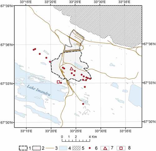
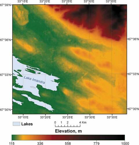
The town is located between Lake Imandra and the Khibiny Mountains. The terrain is hilly. The highest point of the surface topography within the town boundaries is 178.3 m, and the bottom is 129.0 m (Figure 2).

Figure 2. ASTER digital elevation model.

Legend: 1 – according to AWS; 2 – at the WMO station; 3 and 4 – periods with the stable stratification of the lower atmosphere; 3 – wind speed is less than 2 m/s; 4 – wind speed is 0 m/s.

At the latitude of the town of Apatity the polar night lasts from 15 to 28 December. The average air temperature in January–February ranges from −13°C to −15°C. The prevailing wind directions are from the mountains during the cold season. At the same time, complete calm weather events are also frequent during the polar night. The air temperature experiences a radiative cooling-induced drop to −20°C–−30°C in condition of calm weather (Figure 3

Figure 3. Air temperature variations. The arrow indicates the long period of calm weather under astronomical polar night conditions.

). Such low temperatures fall outside the zone of human bioclimatic comfort, so protective measures are needed to restore the feeling of human comfort.

Legend: 1 – according to AWS; 2 – at the WMO station; 3 and 4 – periods with the stable stratification of the lower atmosphere; 3 – wind speed is less than 2 m/s; 4 – wind speed is 0 m/s. The arrow indicates the long period of calm weather under astronomical polar night conditions

2.2. Datasets

Sixteen scenes of infrared thermal band Landsat images (Table 1) acquired under cloudless conditions were selected from the satellite data archives. Next, T_S(x,y), the temperature of snow-covered land surface, was retrieved using a single-channel method (Yu, Guo, and Wu 2014).

Table 1. Satellite data.^a

No	Satellite	Date	Time GMT	Sun elevation, deg	Wind(m/s)	Cloudiness	$T_a^{\hspace{0.17em}}(x_{\mathit{WMO}},y_{\mathit{WMO}})$ ^oC
1	Landsat 8	05.01.2020	18:32	“Night”, Sun elevation < 6	2	0.25	−14.7
2	Landsat 8	24.04.2019	18:32		1	0.60	4.5
3	Landsat 7	02.03.2019	18:32		0	0	−25.0
4	Landsat 8	31.01.2017	09:21		2	0.50	−11.3
5	Landsat 8	03.02.2019	09:14		0	0.20	−31.1
6	Landsat 8	06.02.2019	09:21		2	0.25	−21.7
7	Landsat 8	11.02.2021	09:21	“Day”, Sun elevation < 6	1	0.35	−21.0
8	Landsat 8	18.02.2021	09:27		0	0.25	−15.8
9	Landsat 8	22.10.2014	09:21		1	0.50	−9.2
10	Landsat 8	22.02.2019	09:21		1	0.50	−12.2
11	Landsat 8	01.03.2016	09:21		0	0.25	−15.3
12	Landsat 8	03.03.2019	09:15		0	0.30	−18.7
13	Landsat 7	06.03.2018	09:15		1	1	−15.7
14	Landsat 8	07.03.2018	09:15		0	0.30	−18.0
15	Landsat 8	08.03.2021	09:15		1	0.25	−20.0
16	Landsat 7	08.03.2018	09:17		0	0.80	−24.6

^a$T_a^{\hspace{0.17em}}(x_{\mathit{WMO}},y_{\mathit{WMO}})$ – for the moment of satellite shooting.

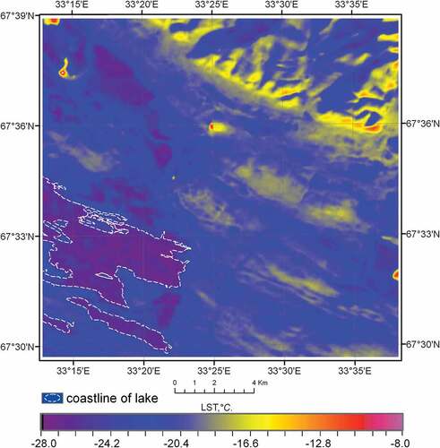
Figure 4 presents an example of T_S(x,y) map retrieved from satellite data ~ 09:00 (GMT), 07.03.2018. As can be seen from Figure 4, T_S(x,y) varied from −28°C to −14°C within the study area.

Figure 4. Map of T_S(x,y) – the land surface temperature retrieved from Landsat 8 satellite image. Time: ~09:00 GMT; Date: 07.03.2018.

Legend: 1 – “Night”; 2 – “Day”(a) WMO data and Landsat data for different times of the day.Legend: 1 – the Lake Imandra shore (WMO); 2 – the hilltop (AWS, see Figure 1).(b) Air temperature (logger and AWS) and surface temperature (Landsat) for different relief altitudes.

A ground-based T_a(x,y) observational network established at the test site (Konstantinov, Grishchenko, and Varentsov 2015; Varentsov et al. 2018) is shown in Figure 1.

The observational network consisted of 21 small temperature sensors (iButton loggers) (0.5°C sensitivity) deployed at locations with coordinates x_j,y_j and a Davis Vantage Pro 2 AWS (0.5°C sensitivity) installed at the site with coordinates x_AWS,y_AWS (Figure 1). Air temperature measurements by the loggers and AWS were made every hour from 25 December 2017 to 2 April 2018. Availability of a ground-based air temperature monitoring network was another reason for choosing Apatity as a test site for the development and verification of the T_a(x,y) satellite mapping technique proposed.

The WMO station (ID WMO 22213) is located near the town of Apatity on the shore of the Lake Imandra (Figure 1). The air temperature data $T_a\left(x_{\mathit{WMO}},y_{\mathit{WMO}}\right)$ at the WMO station in Apatity were sampled at 6 h intervals and used for air temperature mapping only. Data recorded by the loggers and observed from the AWS were employed both for analyzing the air temperature variations at the test site and for evaluating the errors of the T_a(x,y) satellite mapping technique, but not for mapping.

2.3. Backgrounds of the Method

Joint analysis of air temperatures, recorded by the loggers (T_a(x_j,y_j); j is the logger number and $T_a\left(x_{\mathit{WMO}},y_{\mathit{WMO}}\right)$, recorded by the WMO (Figure 5(a)), and the satellite data revealed a strong correlation between T_a(x_j,y_j), $T_a\left(x_{\mathit{WMO}},y_{\mathit{WMO}}\right)$, and T_S(x,y). This is a weakly time-dependent linear correlation which, however, may depend on other factors, as exemplified by Figure 5(b) which demonstrates the regression slope dependence on the relief altitude.

Figure 5. Correlation between the air temperature and the surface temperature. Temperature data in the plots are those observed at the satellite shooting moments indicated in Table 1.

Figure 3 shows extremely low air temperatures that were observed under the polar night conditions during periods of almost complete calm weather. It is worth mentioning that the air temperature at the shore of Lake Imandra (WMO weather station) is by about −10°C lower than that at the highest point in the town of Apatity (see Figures 1 and 3). Moreover, it can be easily seen that this temperature difference is reached rather quickly, whereupon the wind stops and remains approximately constant throughout the calm period. By contrast, under strong wind conditions the air temperatures in the entire territory level off throughout the area, approaching the air temperature at the WMO station (see Figure 3), so air temperature mapping is a trivial task in this case.

The concept underlying the T_a(x,y) satellite mapping technique implies integration of spatial satellite information with the time series of $T_a\left(x_{\mathit{WMO}},y_{\mathit{WMO}}\right)$, observed by WMO weather station (Kritsuk et al. 2019). To justify this technique, we presented the air temperatures at the weather station for each day of satellite imagery as Equation (1)(1) $\begin{array}{rl}& \mathit{Ta}\left(x_{\mathit{WMO}},y_{\mathit{WMO}},{\tau }_i\right)\\ & =\left[T_a\left(x_{\mathit{WMO}},y_{\mathit{WMO}},{\tau }_1\right),\dots T_a\right.\\ & \left(x_{\mathit{WMO}},y_{\mathit{WMO}},{\tau }_k\right),\dots T_a\\ & \left.\left(x_{\mathit{WMO}},y_{\mathit{WMO}},{\tau }_N\right)\right]\end{array}$(1) :

(1) $\begin{array}{rl}& \mathit{Ta}\left(x_{\mathit{WMO}},y_{\mathit{WMO}},{\tau }_i\right)\\ & =\left[T_a\left(x_{\mathit{WMO}},y_{\mathit{WMO}},{\tau }_1\right),\dots T_a\right.\\ & \left(x_{\mathit{WMO}},y_{\mathit{WMO}},{\tau }_k\right),\dots T_a\\ & \left.\left(x_{\mathit{WMO}},y_{\mathit{WMO}},{\tau }_N\right)\right]\end{array}$(1)

where τ_i is the time of satellite shooting, i = 1, … k, …,N is the satellite scene number, N is the number of satellite scenes that were used (16 in our case, according to Table 1), and $T_a\left(x_{\mathit{WMO}},y_{\mathit{WMO}},{\tau }_i\right)$ is the air temperature at the weather station at the time of the i-th satellite shooting.

Further, we constructed a linear regression $T_a\left(x_{\mathit{WMO}},y_{\mathit{WMO}},{\tau }_i\right)$, which are the air temperatures observed at the weather station at the moments of i-th satellite survey, on $T_S\left(x_{\mathit{WMO}},y_{\mathit{WMO}},{\tau }_i\right)=$ $\left[T_S\left(x_{\mathit{WMO}},y_{\mathit{WMO}},{\tau }_1\right),\dots T_S\left(x_{\mathit{WMO}},y_{\mathit{WMO}},{\tau }_k\right),\dots T_S\right.$ $\left.\left(x_{\mathit{WMO}},y_{\mathit{WMO}},{\tau }_N\right)\right]$, representing the surface temperatures at the weather station, mapped by satellite during each of i = 1, … k, ….,N surveys, and obtained Equation (2)(2) $\mathit{Ta}\left(x_{\mathit{WMO}},y_{\mathit{WMO}},\mathit{\tau }\right)=\mathit{A}\times T_S\left(x_{\mathit{WMO}},y_{\mathit{WMO}},\mathit{\tau }\right)+\mathit{B}$(2) :

(2) $\mathit{Ta}\left(x_{\mathit{WMO}},y_{\mathit{WMO}},\mathit{\tau }\right)=\mathit{A}\times T_S\left(x_{\mathit{WMO}},y_{\mathit{WMO}},\mathit{\tau }\right)+\mathit{B}$(2)

where A and B are the regression coefficients calculated for the pixel x_WMO,y_WMO of the WMO weather station.

Equation (2)(2) $\mathit{Ta}\left(x_{\mathit{WMO}},y_{\mathit{WMO}},\mathit{\tau }\right)=\mathit{A}\times T_S\left(x_{\mathit{WMO}},y_{\mathit{WMO}},\mathit{\tau }\right)+\mathit{B}$(2) makes it possible to estimate the air temperature at any pixel of the map from the surface temperature. Coefficients A and B in Equation (2)(2) $\mathit{Ta}\left(x_{\mathit{WMO}},y_{\mathit{WMO}},\mathit{\tau }\right)=\mathit{A}\times T_S\left(x_{\mathit{WMO}},y_{\mathit{WMO}},\mathit{\tau }\right)+\mathit{B}$(2) are taken constant in time for the entire study area. This is because the snow-covered surface is mostly homogeneous, so the technique is developed for calm weather conditions, when no turbulent heat transfer occurs between the land surface and the atmosphere (Figure 3).

Next, the second linear regression $T_S\left(x_{\mathit{WMO}},y_{\mathit{WMO}},{\tau }_i\right)$ on $T_a\left(x_{\mathit{WMO}},y_{\mathit{WMO}},{\tau }_i\right)$ for each pixel of the map being compiled was constructed as Equation (3)(3) $T_S\left(\mathit{x},\mathit{y},\mathit{\tau }\right)=\mathit{C}(\mathit{x},\mathit{y})\times T_a\left(x_{\mathit{WMO}},y_{\mathit{WMO}},\mathit{\tau }\right)+\mathit{D}\left(\mathit{x},\mathit{y}\right)$(3)

(3) $T_S\left(\mathit{x},\mathit{y},\mathit{\tau }\right)=\mathit{C}(\mathit{x},\mathit{y})\times T_a\left(x_{\mathit{WMO}},y_{\mathit{WMO}},\mathit{\tau }\right)+\mathit{D}\left(\mathit{x},\mathit{y}\right)$(3)

Equation (3)(3) $T_S\left(\mathit{x},\mathit{y},\mathit{\tau }\right)=\mathit{C}(\mathit{x},\mathit{y})\times T_a\left(x_{\mathit{WMO}},y_{\mathit{WMO}},\mathit{\tau }\right)+\mathit{D}\left(\mathit{x},\mathit{y}\right)$(3) represents the spatial distribution of the relationship T_S(x,y,τ) on $T_a\left(x_{\mathit{WMO}},y_{\mathit{WMO}},\mathit{\tau }\right)$. Substituting (2) into (3) and extending (3) to the entire test site gives Equation (4)(4) $T_a\left(\mathit{x},\mathit{y},\mathit{\tau }\right)=\mathit{F}\left(\mathit{x},\mathit{y}\right)\times T_a\left(x_{\mathit{WMO}},y_{\mathit{WMO}},\mathit{\tau }\right)+\mathit{G}\left(\mathit{x},\mathit{y}\right)$(4)

(4) $T_a\left(\mathit{x},\mathit{y},\mathit{\tau }\right)=\mathit{F}\left(\mathit{x},\mathit{y}\right)\times T_a\left(x_{\mathit{WMO}},y_{\mathit{WMO}},\mathit{\tau }\right)+\mathit{G}\left(\mathit{x},\mathit{y}\right)$(4)

Where $\mathit{F}\left(\mathit{x},\mathit{y}\right)=\mathit{A}\times \mathit{C}(\mathit{x},\mathit{y});\mathit{G}\left(\mathit{x},\mathit{y}\right)=\mathit{A}\times \mathit{D}\left(\mathit{x},\mathit{y}\right)+\mathit{B}$.

The correlation analysis revealed a strong relationship (correlation coefficient > 0.9) between $T_a\left(x_{\mathit{WMO}},y_{\mathit{WMO}}\right)$ and T_S(x,y) in conditions of calm weather (Figure 6). However, the slopes of regressions are different for each point (pixel) of the mapping area (Figure 7(a)). This is the fundamental criterion of applicability of satellite technique of air temperature mapping during the polar night.

Figure 6. Map of R(x,y) – coefficients of correlation between T_S(x,y,τ) (Landsat) and $T_a\left(x_{\mathit{WMO}},y_{\mathit{WMO}},{\tau }_i\right)$; τ_i is the time of i-th satellite shooting. Date: 01.02.2018.

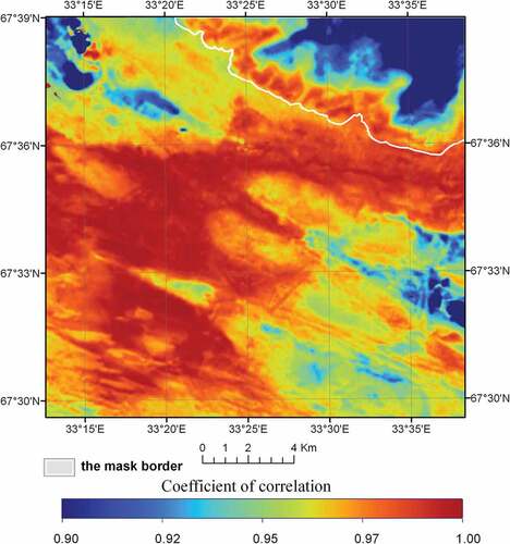
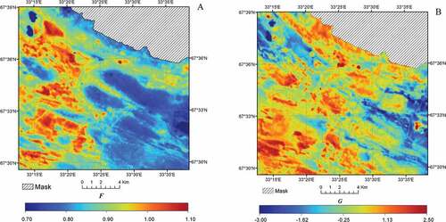
Figure 7. Maps of coefficients of Equation (4)(4) $T_a\left(\mathit{x},\mathit{y},\mathit{\tau }\right)=\mathit{F}\left(\mathit{x},\mathit{y}\right)\times T_a\left(x_{\mathit{WMO}},y_{\mathit{WMO}},\mathit{\tau }\right)+\mathit{G}\left(\mathit{x},\mathit{y}\right)$(4) , compiled from the results of multiple satellite imagery (Table 1) and of the standard observations at WMO 22213 weather station.

(a) Map of coefficient F(x,y).(b) Map of coefficient G(x,y).

As can be seen in Figure 6, in the mountainous part of the test site with elevations exceeding 800 m (upper right corner) the correlation coefficients are less than 0.9. Therefore, this area was masked on the other maps.

Equation (4)(4) $T_a\left(\mathit{x},\mathit{y},\mathit{\tau }\right)=\mathit{F}\left(\mathit{x},\mathit{y}\right)\times T_a\left(x_{\mathit{WMO}},y_{\mathit{WMO}},\mathit{\tau }\right)+\mathit{G}\left(\mathit{x},\mathit{y}\right)$(4) shows the relationship between the air temperature at the WMO station and that at any point in the study area. From (4) it follows that knowledge of $T_a\left(x_{\mathit{WMO}},y_{\mathit{WMO}},\mathit{\tau }\right)$ allows mapping the air temperature, even if τ is not equal to τ_i, i.e. at a time when satellite shooting has not been carried out, but only provided that calm weather conditions are observed. However, the corresponding satellite image time must be chosen from the time interval lying between the time points of taking the first and the last satellite images, whose data were used to construct Equation (3)(3) $T_S\left(\mathit{x},\mathit{y},\mathit{\tau }\right)=\mathit{C}(\mathit{x},\mathit{y})\times T_a\left(x_{\mathit{WMO}},y_{\mathit{WMO}},\mathit{\tau }\right)+\mathit{D}\left(\mathit{x},\mathit{y}\right)$(3) .

Figure 7 presents the maps of the coefficients of Equation (4)(4) $T_a\left(\mathit{x},\mathit{y},\mathit{\tau }\right)=\mathit{F}\left(\mathit{x},\mathit{y}\right)\times T_a\left(x_{\mathit{WMO}},y_{\mathit{WMO}},\mathit{\tau }\right)+\mathit{G}\left(\mathit{x},\mathit{y}\right)$(4) . The clearly visible spatial heterogeneity of the coefficient compiled may be caused by the nonuniform distribution of the cooling mechanisms over the study area due to radiative cooling and, as was discussed in (Demin et al. 2018; Demin 2019), to cold air drainage from hills to lowlands. That is why the direct application of the regression technique to the entire study area, as was done in (Zhu, Lű, and Jia 2013; Ho et al. 2014) should give larger errors than the use of Equation (4)(4) $T_a\left(\mathit{x},\mathit{y},\mathit{\tau }\right)=\mathit{F}\left(\mathit{x},\mathit{y}\right)\times T_a\left(x_{\mathit{WMO}},y_{\mathit{WMO}},\mathit{\tau }\right)+\mathit{G}\left(\mathit{x},\mathit{y}\right)$(4) .

3. Results

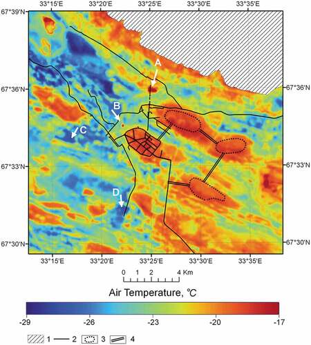
One of the main results of this study was the possibility to compile the air temperature map for the Apatity test site (for the air temperature at WMO22213 of −25.4°C (Figure 8)). The T_a(x,y) values mapped with the greatest confidence lie in the range between −27°C and −17°C (Figure 8).

Figure 8. Map of air temperature, compiled on the base of the satellite and WMO weather station data. Time: 00:00 GMT; 01.02.2018. This time is between the times of satellite surveys (see Table 1).

Legend: 1 – mask; 2 – roads; 3 – proposed new districts; 4 – proposed highways interconnecting the new districts. A - CHP plant; B - municipal wastewater treatment plant; C and D – lowlands.

Legend: 1 – mask; 2 – roads; 3 – proposed new districts; 4 – proposed highways interconnecting the new districts.

The map was compiled according to Equation (4)(4) $T_a\left(\mathit{x},\mathit{y},\mathit{\tau }\right)=\mathit{F}\left(\mathit{x},\mathit{y}\right)\times T_a\left(x_{\mathit{WMO}},y_{\mathit{WMO}},\mathit{\tau }\right)+\mathit{G}\left(\mathit{x},\mathit{y}\right)$(4) , to which end the time series of the air temperatures at the meteorological station $T_a\left(x_{\mathit{WMO}},y_{\mathit{WMO}},\mathit{\tau }\right)$ and the land surface temperatures reconstructed from the thermal space imagery T_S(x,y,τ) were used only (see Table 1). Importantly, the air temperatures recorded by the loggers were not used for surface air temperature mapping. Rather, they were used only for estimating the errors of satellite mapping of air temperature based on independent measurements (direct validation) (see Supplemental Materials).

The first stage of verification of the proposed T_a(x,y,τ) mapping technique consisted in the instrumental assessment of the quality of the scenes used for constructing regressions (2)–(4), to which end a cross-validation procedure was applied. The revealed negligible differences between the air temperatures obtained with the use of the sets of six and five scenes are indicative of the lack of major interferences in the case of the scenes selected (see Supplemental materials). Also, factors affecting the mapping errors were studied. Among them, the relief altitude was identified as the major contributor to the air temperature mapping errors. Specifically, the mapping errors were found to increase with altitude (see Supplemental Materials).

Importantly, the date and time for which this map was compiled (Time: 00:00 GMT; Date: 01.02.2018) are different from those of the Landsat 8 satellite passing over the test site. In this respect the novel technique compares advantageously with the approaches employing direct correlations with crowd-sourced hour-synchronous air temperature observations like those reported in (Srivanit and Hokao 2012; Ho et al. 2014; Zhu, Lű, and Jia 2013; Williamson et al. 2014; Venter et al. 2020).

The T_a(x,y,τ) mapping errors were estimated by the following procedure. Within the polar night period (15 to 28 December) extended by incorporation of the days that followed on which the Sun elevation was no greater than 6° we selected four intervals during which calm and clear weather conditions appropriate for satellite imagery collection were observed. These time intervals comprised a total 16 observation times for which the air temperature measurements at the Apatity meteorological station (WMO 22213) were available in the public domain. On this basis the T_a(x,y,τ) values at the 16 different observation times were calculated for each logger and the AWS (22 control points). This gave a total of 300 T_a(x,y,τ) values that were compared with the T_a(x_j,y_j,τ) data recorded by the loggers. Next, by using the standard formulas the accuracy and precision of air mapping under dead-calm conditions were estimated as σ = 1.5°C and δ = 1.0°C, respectively (see Table SM.2 in Supplemental Materials).

For better statistical validity of the estimated the errors, the time periods during which the wind speeds did not exceed 2 m/s were also included in the error estimation procedure, alongside the periods of dead calm. Consequently, the number of observation times increased to 38, which, considering the 22 control points available (loggers and AWS locations), gave 836 control measurements. As a result, the systematic error (precision) was reduced to δ = 1.8°C, while the root mean square error (accuracy) increased to σ = 2.3°C (see Table SM.2 in Supplemental Materials).

4. Discussion

Detailed error analysis revealed the growth of the root-mean-square error σ depending on the relief altitude (Figure 9).

Figure 9. Dependence of errors σ on the relief altitude.

A more in-depth detailed analysis of factors such as vegetation and anthropogenic heat flux showed that they have only a slight impact on the T_a(x_j,y_j,τ) mapping errors (see Supplemental Materials).

Importantly, the temperature sensitivity of the loggers was 0.5°C. Besides, the real temperature sensitivity of the infrared thermal images of the Landsat satellites, due to atmosphere absorption and a very low snow surface temperature, was no better than 0.5°C. Therefore, the estimated errors of air temperature satellite mapping technique can be considered as satisfactory enough for solving practical tasks of analyzing the spatial patterns of thermal microclimate in the polar night conditions.

An analysis of the T_a(x,y) map compiled by using the technique proposed shows that, at 00:00 GMT, 01.02.2018, the air temperature within the study area was strongly heterogeneous, ranging from −10°C to below −30°C. The highest T_a(x,y) values are mapped at the tops of the hills (see Figures 2 and 8). The largest local T_a(x,y) values correspond to the location sites of the CHP plant (point A in Figure 8) and the municipal wastewater treatment plants (point B in Figure 8). Minimum temperatures were recorded at the Lake Imandra nearby lowlands (points C and D in Figure 8).

A visual comparison of the T_a(x,y) map (Figure 8) with the digital elevation model (Figure 2) shows that elevations are characterized by higher T_a(x,y) values than lowlands.

Possible physical mechanisms of this phenomenon were previously studied at the Polar Geophysical Institute of Kola Scientific Center of RAS, in particular, via continuous measurements of the air temperature with a sensor installed on the roof of a car (Shumilov, Kasatkina, and Kanatjev 2017). In that work, it was concluded that one possible reason for the phenomenon observed is the so-called “relief effect”, consisting in that cold (heavy) air from elevations “slithers” into low landforms. Alongside this mechanism, strong radiative cooling in conditions of a cloudless sky and calm weather may be observed. As a result, the air temperature rises as the altitude from the land surface increases to several hundred meters. Consequently, during the polar night the atmosphere heats the hills stronger than the lowlands. Importantly, the elevation difference in the study area exceeds 150 m, so the formation of the pattern observed could be driven by the radiative cooling mechanism.

Of particular note is that the resultant T_a(x,y,τ) map (Figure 8) allows us to justify the approach to solving some practical problems of providing environmental safety, e.g. that of evaluating the bioclimatic comfort for the population of the Arctic zone. Specifically, at 00:00 GMT, 01.02.2018, T_a(x,y,τ) changed from −12°C at the top of the hill in the southeast corner of the Apatity town to −32°C on the shore of the frozen Lake Imandra (points C and D in Figure 8). Thus, the decrease in T_a(x,y,τ) reached −20°C at the distance of about 5 km. Such significant changes in T_a(x,y,τ) may adversely affect the bioclimatic sensation of the local people when moving from a “warm” area to an overcooled one. Moreover, there exists a strong correlation between the T_a(x,y) reduction and the energy spent for house heating (Varentsov et al. 2018). Therefore, from the energy efficiency perspective and for reasons of the population health protection, city planning on the hills seems to be the most efficient option to be adopted for the Arctic region. Thus, a possible principal architecture of new districts on the hill, interconnected by roads passing through the lowlands, can be proposed for the Apatity town (see 3 and 4 in the legend of Figure 8). Each of these areas should be planned in a semi-autonomous manner in order to minimize the need for residents to cross the overcooled lowlands between the areas.

At present, the main distinguishing quantitative feature of a megalopolis is its large population of more than 10 million inhabitants. As to the main qualitative feature of this largest settlement, this is its internal structure, historically formed by the pooled original settlements interconnected by the transport network (Gorkin 2006). That is why the future Arctic cities, if projected on the hills as several local areas interlinked by transportation routes to be laid in the lowlands, can be called “Arctic megalopolises” because of their internal structure specific to megalopolises. However, in the case of “Arctic megalopolises”, this structure would be the result of the climatic specificity of the polar territories rather than the historical merger of individual settlements.

5. Conclusions

1. A technique was developed for air temperature mapping via fusion of spatial information derived from satellite imagery with the time series of air temperature observations by standard weather stations (WMO).

2. The novel technique is based on the construction of linear regressions relating the air temperature at a WMO station with the land surface temperature in each pixel of the digital map. The regression parameters are different for different pixels of the map.

3. The developed novel technique of satellite mapping of air temperature is only applicable during the polar night period in cloudless and windless conditions.

4. An advantage offered by the technique is the possibility to map the air temperature for dates and times when satellite imagery has not been carried out. This is highly beneficial in terms of providing daily data unavailable from high-resolution thermal satellite imagery by modern Landsat and Terra (ASTER) satellites because of its low repeatability.

5. The errors of the novel high-spatial-resolution satellite-based air temperature mapping technique are satisfactory enough for solving some practical tasks related to bioclimatic comfort evaluation for the population in the Arctic region.

6. The implementation of this novel technique on the example of the town of Apatity during the polar night period, in clear and calm weather conditions, showed that the air temperature on the elevations of surface relief was higher than in the lowlands. This temperature difference must be considered when planning new large cities during the upcoming development of the Arctic. Specifically, it is advisable that new large polar settlements be designed on positive forms of surface topography as a system of maximally autonomous sub-districts interconnected by highways. Such architecture can provide more comfortable bioclimatic conditions for the population, as well as energy saving for house heating systems. Cities constructed according to this principle can be called “Arctic megalopolises.”

Disclosure statement

No potential conflict of interest was reported by the author(s). V.Gornyy , S. Kritsuk , T. Davidan , I. Latypov , A. Manvelova , A. Tronin., and M.Vasiliev – theoretical bases of novel method, satellite data processing and analyses. P.Konstantinov. M. Varentsov – installation of logger and AWS network and air temperature long time observation, processing, and quality control.

Data availability statement

The raw land surface temperature data can be obtained from the LAADS DAAC – NASA (Level-1 and Atmosphere Archive and Distribution System Web Interface). https://ladsweb.modaps.eosdis.nasa.gov

Supplementary material

Supplemental data for this article can be accessed here

Additional information

Funding

The investigation was supported by SRCES RAS, by the project TRAKT 2018, by Belmont Forum project SERUS, and RFBR project no. 20-55-71004. Pre-processing of in-situ observations in Apatity performed by Mikhail Varentsov and Pavel Konstantinov was supported by Russian Science Foundation, project no. 19-05-50112. Results of this research are promoted through the activities of the PanEurasian EXperiment (PEEX) programme. We are grateful to Dr. Igor Esau for insightful discussions.

Notes on contributors

Kritsuk Sergei

Sergei Kritsuk is a senior researcher in Saint-Petersburg Scientific Research Center for Ecological Safety, Russian Academy of Sciences (SRCES RAS). He received his Master degree in exploration geophysics from Leningrad Mining Institute and applied mathematics from Leningrad State University. His major scientific interest is remote sensing.

Victor Gornyy

Victor Gornyy is the Head of Remote sensing and Geo-Informatics laboratory in SRCES RAS. He received his MS (exploration geophysics) and PhD (exploration geophysics) from Leningrad Mining Institute. His major scientific interests are remote sensing, geothermy and environment safety.

Tatiana Davidan

Tatiana Davidan is a leading engineer in SRCES RAS. Her major scientific interest is remote sensing data processing.

Iscander Latypov

Iscander Latypov is a senior researcher. He received his MS (mathematics) from Kazan University, and PhD (mathematics) from Leningrad State University. His major scientific interest is inverse problem solutions in remote sensing, including ill-posed problems.

Alexandra Manvelova

Alexandra Manvelova is a researcher in SRCES RAS. She received her master degree in geography from Saint-Petersburg State University. Her Major scientific interests are economical geography and environment protection.

Pavel Konstantinov

Pavel Konstantinov is an assistant professor in Moscow State University. He received his PhD in Geography. His major scientific interest is urban microclimate.

Andrei Tronin

Andrei Tronin is the director of SRCES RAS. He received his MS (exploration geophysics) from Leningrad Mining institute, PhD (geophysics) from Schmidt Institute of Physics of the Earth, and DrScs from Saint-Petersburg State University. His major scientific interests are remote sensing, seismology and environment protection.

Mikhail Varentsov

Mikhail Varentsov is a researcher in Moscow State University. His major scientific interest is application of supercomputer to microclimate problem solution.

Mikhail Vasiliev

Mikhail Vasiliev is a senior researcher in Moscow State University. His major scientific interest is application of supercomputer to microclimate problem solution.

References

- Bornshtein, R.D. 1968. “Observation of Urban Heat Island Effect in New York City.” Journal of Applied Meteorology Aug 1968: 575–582. doi:10.1175/1520-0450(1968)007<0575:OOTUHI>2.0.CO;2.
- Chapman, L., J.E. Thornes, and A.V. Bradley. 2001. “Modeling of Road Surface Temperature from a Geographical Parameter Database. Part 1: Statistical.” Meteorological Applications 8 (4): 409–419. doi:10.1017/S1350482701004030.
- Cotton, W.R., and R.A. Pielke. 2007. Human Impacts on Weather and Climate. Cambridge: Cambridge University Press.
- Cracknell, A.P., and Y. Xue. 1996. “Thermal Inertia Determination from Space − a Tutorial Review.” International Journal of Remote Sensing 17 (3): 431–461. doi:10.1080/01431169608949020.
- Demin, V.I., B.V. Kozelov, A.P. Sobakin, Y.V. Menshov, and Y.A. Gorban. 2018. “Influence of the Microclimate on the Results of Urban Heat Island Modeling (On the Example of the Town of Apatity).” Mathematical Studies in the Natural Sciences. Proceedings of the XV All-Russian Scientific School 15: 65–78.
- Demin, V.I. 2019. “Role of Anthropogenic and Natural Drivers in the Estimation of Urban Heat Island.” Current Problems in Remote Sensing of the Earth from Space 16 (5): 25–33. doi:10.21046/2070-7401-2019-16-5-25-33.
- Gorkin, A. 2006. Geography: Modern Illustrated Encyclopedia. Moscow: Rosmen.
- Gornyy, V.I., S.G. Kritsuk, I.S. Latypov, A.A. Tronin, A.V. Kiselev, O.V. Brovkina, V.E. Filippovich, S.A. Stankevich, and N.S. Lubsky. 2017. “Thermophysical Properties of the Surface of Urban Environment (Based on Satellite Imagery of St. Petersburg and Kiev).” Current Problems in Remote Sensing of the Earth from Space 14 (3): 51–66.
- Hinkel, K.M., F.E. Nelson, A.E. Klene, and J.H. Bell. 2003. “The Urban Heat Island in Winter at Barrow, Alaska.” International Journal of Climatology 23 (15): 1889–1905. doi:10.1002/joc.971.
- Ho, H.C., A. Knudby, P. Sirovyak, Y. Xu, M. Hodul, and S.B. Henderson. 2014. “Mapping Maximum Urban Air Temperature on Hot Summer Days.” Remote Sensing of Environment 154: 38–45. doi:10.1016/j.rse.2014.08.012.
- Huang, B., and J. Wang. 2020. “Big Spatial Data for Urban and Environmental Sustainability.” Geo-spatial Information Science 23 (2): 125–140. doi:10.1080/10095020.2020.1754138.
- Im, U., J.H. Christensen, O.K. Nielsen, M. Sand, R. Makkonen, C. Geels, C. Anderson, J. Kukkonen, S. Lopez-Aparicio, and J. Brandt. 2019. “Contributions of Nordic Anthropogenic Emissions on Air Pollution and Premature Mortality over the Nordic Region and the Arctic.” Atmospheric Chemistry and Physics 19 (20): 12975–12992. doi:10.5194/acp-19-12975-2019.
- Konstantinov, P.I., M.Y. Grishchenko, and M.I. Varentsov. 2015. “Mapping Urban Heat Islands of Arctic Cities Using Combined Data on Field Measurements and Satellite Images Based on the Example of the City of Apatity (Murmansk Oblast).” Izvestiya, Atmospheric and Oceanic Physics 51 (9): 992–998. doi:10.1134/S000143381509011X.
- Konstantinov, P., M. Varentsov, and I. Esau. 2018. “A High Density Urban Temperature Network Deployed in Several Cities of Eurasian Arctic.” Environmental Research Letters 13 (7): 075007. doi:10.1088/1748-9326/aacb84.
- Koppe, C., S. Kovats, G. Jendritzky, and B. Menne. 2004. “Heat-Waves: Risks and Responses.” Health and Global Environmental Change Series 2. http://www.euro.who.int/globalchange
- Kritsuk, S.G., V.I. Gornyy, I.S. Latypov, A.A. Pavlovskii, and A.A. Tronin. 2019. “Satellite Risk Mapping of Urban Surface Overheating (By the Example of Saint Petersburg).” Current Problems in Remote Sensing of the Earth from Space 16 (5): 34–44. LAADS DAAC, NASA (Level-1 and Atmosphere Archive and Distribution System Web Interface). https://ladsweb.modaps.eosdis.nasa.gov
- Magee, N., J. Curtis, and G. Wendler. 1999. “The Urban Heat Island Effect at Fairbanks, Alaska.” Theoretical and Applied Climatology 64 (1): 39–47. doi:10.1007/s007040050109.
- Park, M., S. Park, C. Jung-Hoon, C. Min-Hyeok, S. Yunyoung, and K. Minsoo. 2017. “High-Resolution Urban Observation Network for a User-Specific Meteorological Information Service in the Seoul Metropolitan Area, Korea.” Atmospheric Measurement Techniques Discussions 10 (4): 1575–1594. doi:10.5194/amt-10-1575-2017.
- Ruuhela, R., A. Votsis, J. Kukkonen, K. Jylhä, S. Kankaanpää, and A. Perrels. 2021. “Temperature-Related Mortality in Helsinki Compared to Its Surrounding Region over Two Decades, with Special Emphasis on Intensive Heatwaves.” Atmosphere 12 (1): 46. doi:10.3390/atmos12010046.
- Ruuhela, R., K. Jylhä, T. Lanki, P. Tiittanen, and A. Matzarakis. 2017. ““Biometeorological Assessment of Mortality Related to Extreme Temperatures in Helsinki Region, Finland, 1972–2014”.” International Journal of Environmental Research and Public Health 14 (8): 944. doi:10.3390/ijerph14080944.
- Schwarz, N., S. Lautenbach, and R. Seppelt. 2011. “Exploring Indicators for Quantifying Surface Urban Heat Islands of European Cities with MODIS Land Surface Temperatures.” Remote Sensing of Environment 115: 3175–3186. doi:10.1016/j.rse.2011.07.003.
- Shumilov, O.I., E.A. Kasatkina, and A.G. Kanatjev. 2017. “Urban Heat Island Investigations in Arctic Cities of Northwestern Russia.” Journal of Meteorological Research 31 (6): 1161–1166. doi:10.1007/s13351-017-7048-8.
- Srivanit, M., and K. Hokao. 2012. “Thermal Infrared Remote Sensing for Urban Climate and Environmental Studies: An Application for the City of Bangkok, Thailand.” Journal of Architectural/Planning Research and Studies 9 (1): 83–100.
- Varentsov, M., P. Konstantinov, A. Baklanov, I. Esau, V. Miles, and R. Davy. 2018. “Anthropogenic and Natural Drivers of a Strong Winter Urban Heat Island in a Typical Arctic City.” Atmospheric Chemistry and Physics 18 (23): 17573–17587. doi:10.5194/acp-2018-569.
- Venter, Z.S., O. Brousse, I. Esau, and F. Meier. 2020. “Hyperlocal Mapping of Urban Air Temperature Using Remote Sensing and Crowd Sourced Weather Data.” Remote Sensing of Environment 242: 111791. doi:10.1016/j.rse.2020.111791.
- Williamson, S.N., D.S. Hik, J.A. Gamon, J.L. Kavanaugh, and G.E. Flowers. 2014. “Estimating Temperature Fields from MODIS Land Surface Temperature and Air Temperature Observations in a Sub-Arctic Alpine Environment.” Remote Sensing of Environment 6 (2): 946–963. doi:10.3390/rs6020946.
- Xu, K., and Y. Wang. 2021. “Analysis of Atmospheric Temperature Data by 4D Spatial–temporal Statistical Model.” Scientifc Reports 11 (1): 1–9.
- Young, T.K., and T.M. Makinen. 2010. “The Health of Arctic Populations: Does Cold Matter?” American Journal of Human Biology 22: 129–133. doi:10.1002/ajhb.20968.
- Yu, X., X. Guo, and Z. Wu. 2014. “Land Surface Temperature Retrieval from Landsat 8 TIRS—Comparison between Radiative Transfer Equation-Based Method, Split Window Algorithm and Single Channel Method.” Remote Sensing of Environment 6 (10): 9829–9852. doi:10.3390/rs6109829.
- Zhou, D., J. Xiao, B. Stefania, B. Christian, D. Kaveh, Y. Zhou, F. Steve, R. Yao, Z. Qiao, and A. Sobrino José. 2019. “Satellite Remote Sensing of Surface Urban Heat Islands: Progress, Challenges, and Perspectives.” Remote Sensing 11 (1): 48. doi:10.3390/rs11010048.
- Zhu, W., A. Lű, and S. Jia. 2013. “Estimation of Daily Maximum and Minimum Air Temperature Using MODIS Land Surface Temperature Products.” Remote Sensing of Environment 130: 62–73. doi:10.1016/j.rse.2012.10.034.