Increasing spatial coverage in rough terrain and vegetated areas using InSAR optimized pixel selection: application to Tohoku, Japan

ABSTRACT

One of the major limitations of using Interferometric Synthetic Aperture Radar (InSAR) in time series analysis is the low-phase coherence associated with rough terrain and vegetated areas, which results in limited spatial coverage in such regions. Permanent scatterers technique was introduced to overcome this limitation using time-series analysis. However, identifying major scatterers within a pixel requires the single-looked pixels oversampling which can be a demanding process especially with large interferometric stacks and vast study areas. Therefore, using multilooked temporal coherent pixels was proposed to increase processing efficiency and coverage by utilizing distributed targets, but this technique may exclude pixels with reliable phase returns because of their temporal varying neighboring pixels. In this paper, we propose a technique to identify multilooked temporal stable pixels with reliable phase returns independent of their neighboring pixels. We conduct a simulation analysis to relate the spatial coherence of a pixel with its expected temporal correlation in the time series analysis module. We found that a liberal temporal correlation threshold of 0.53 in multilooked pixels stack is equivalent to a spatial coherence threshold of 0.2 when using number of looks of 9, which is considered acceptable in temporal coherent pixels, in terms of phase standard deviation. Applying these findings to study the 2011 Tohoku earthquake in the northeastern part of Japan resulted in increasing the number of usable pixels and spatial coverage index by nearly 50.4% and 36.8%, respectively, compared to the temporal coherent pixels. Furthermore, we propose an approach to integrate GPS observations with InSAR time series analysis, which resulted in deformation maps of the megathrust 2011 Tohoku earthquake with mean RMSE of 11.4 mm and a correlation of 98% in comparison to GPS observations.

KEYWORDS:

• 2011 Tohoku earthquake
• temporal stable pixels
• coherence
• phase noise
• GPS
• coverage index

1. Introduction

For many years, Interferometric Synthetic Aperture Radar (InSAR) has been widely used for estimating surface deformations due to several phenomena such as earthquakes (Massonnet et al. 1994), glacier movements (Goldstein et al. 1993), and land subsidence (Buckley et al. 2003). However, the conventional InSAR analysis has proven to be less appropriate for estimating deformations in rough terrain and vegetated regions, in terms of accuracy, reliability, and spatial coverage, especially when associated with the unprecedented deformation signature of the megathrust 2011 Tohoku earthquake.

In 2011, Japan was struck by an earthquake with a moment magnitude of M9.0, known as the 2011 Tohoku earthquake. This is considered the largest seismic event recorded in Japan. This earthquake and the tsunami that followed caused unprecedented damage along the Pacific Coast in Tohoku and Kanto regions. The coseismic deformation has a maximum horizontal movement of 5.3 m and subsidence of 1.2 m (Imakiire and Kobayashi 2011). Several researchers studied the deformation signature of the megathrust earthquake demonstrating a continuous postseismic motion with varying patterns. Sun et al. (2014) studied the Tohoku region using Global Position System (GPS) observations and numerical modeling. They demonstrated that the surface motion is a consequence of the relaxation of stresses induced by asymmetric rupture of the thrust earthquake. Also, Ohzono et al. (2012) detected an anomalous crustal strain in the Tohoku region associated with a step-like stress change induced by the 2011 Tohoku earthquake.

These findings raised the interest in observing the coseismic and postseismic crustal deformations in north-eastern Japan with fine spatial resolution. ElGharbawi and Tamura (2015) presented a methodology to estimate crustal deformation time series in regions that have been affected by the megathrust earthquake using InSAR and GPS data. This approach uses the unwrapped phase as the basic observation in the estimation process, which generates deformation maps with adequate coverage in Kanto region because of its high interferometric coherence. On the other hand, the Tohoku region, in North-eastern Japan, has vast vegetated areas and rough natural terrain. These signatures cause interferometric phase decorrelation, which reduces the signal coherence and results in unreliable phase unwrapping and low spatial coverage.

To overcome the InSAR temporal decorrelation problem, Ferretti, Prati, and Rocca (2001) introduced Permanent Scatterers InSAR (PS-InSAR). The main idea of PS-InSAR is identifying the interferometric phase of the most stable targets within the pixel, which can be a pole, building corner, or large boulder. This process requires analyzing and oversampling single-look interferometric stack, which can be a computational challenge when applied to large areas. To reduce the computational load of the interferometric analysis, several researchers proposed using multilooked pixels to utilize distributed targets that maintain spatial coherence over the InSAR stack. The distributed targets are identified as the pixels that exhibit homogenous radar backscatter. For example, Mora, Mallorqui, and Broquetas (2003) although their work improved the PS-InSAR analysis procedure, they introduced using spatial coherence as a selection criterion for PS pixels. They suggested using pixels with high spatial coherence in the whole interferometric stack. Zhang, Ding, and Lu (2011) and Zhang et al. (2012) introduced the term Temporal Coherent Pixels (TCP) which they defined as the points that maintain coherence during one or several intervals of SAR acquisitions. They suggested refining the coherent pixels selection using offset deviation and oversampling cross-correlation. Several other researchers used spatial coherence as a selection criterion (e.g. Blanco-Sánchez et al. 2008; Crosetto, Crippa, and Biescas 2005; López-Quiroz et al. 2009; Hetland et al. 2012).

Spatial coherence reflects the correlation between the phase of the desired pixel and the phase of its surroundings within the estimation window, and applying the TCPs technique in multilooked interferograms of vegetated areas reduces the probability of identifying pixels with stable and reliable phase information because of their temporal varying neighboring pixels.

For the aforementioned reasons, we propose a methodology for processing a multilooked interferometric stack to produce deformation time series with high spatial coverage by utilizing Temporal Stable Pixels (TSP) and GPS observations. The basic idea is selecting a suitable temporal phase correlation threshold to increase the number of identified temporal stable pixels, independent of their surroundings while ensuring accurate deformation estimation. To achieve this target, we present a simulation analysis that relates spatial coherence with temporal phase correlation using varying size-estimation windows. This simulation enables us to select a suitable temporal correlation threshold that identifies pixels with phase standard deviation comparable to the expected of pixels selected by a spatial coherence threshold in traditional InSAR analysis. We identify the TSPs as the pixels with temporal phase correlation equivalent to the expected of a pixel having coherence of a suitable threshold. In this study, we selected a threshold of 0.2 (Ferretti et al. 2007; Hagberg, Ulander, and Askne 1995). This resulted in increasing the number of identified pixels by nearly 50.4% compared to pixels with a spatial coherence threshold of (≥ 0.2) for the entire interferometric stack. ElGharbawi and Tamura (2019)presented the first test results of this technique, while in this article we present a detailed illustration of the proposed approach with full analysis results for north-eastern Japan. In addition, we present an approach to combine TSPs and GPS observations to estimate deformation time series with a few millimeters’ accuracy. It must be noted that, because of the several definitions and selection criteria of the TCPs in the literature, in this research, we use the term TCPs to describe a group of pixels that exhibit a spatial coherence higher than or equals 0.2 for the entire InSAR stack.

This paper is organized as follows: Section 2 defines the study region, used data, simulation results, and the main challenges in this analysis. Section 3 illustrated the proposed analysis approach. Section 4 presents the application of the proposed method to the East coast of Japan, and finally Section 5 is dedicated to conclusions.

2. Study region and problem identification

2.1. Study region and data used

In this paper, we focus on measuring the deformation signature of the 2011 Tohoku earthquake over the East coast of Japan (Figure 1), which covers several regions, e.g. Chiba, Iwaki, Sendai, Iwate, and Aomori. Most of these regions contain heavy vegetation cover and characterized by its rough natural terrain, which adds more difficulties to the InSAR analysis.

Figure 1. (a) Study areas, showing the SAR images and GPS stations, base map is a gray shade Digital Elevation Model (DEM), (b) Google earth image showing the vegetation cover.

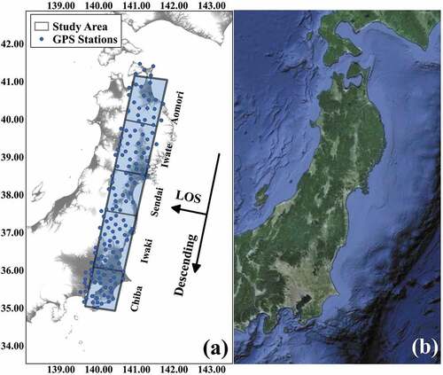
The importance of this analysis is emphasized by the need to measure the detailed deformation signature of the 2011 Tohoku earthquake, coseismic and postseismic, to fully understand this unprecedented event and its effect on future seismic motion. In addition, we integrate InSAR and GPS measurements to estimate land deformation in difficult areas with fine resolution.

In this analysis, we use Synthetic Aperture Radar (SAR) acquisitions and GPS measurements to monitor crustal deformations in the north-eastern part of Japan. SAR images were provided by the European Space Agency © ESA (2014), which were acquired by the ESA’s satellite ENVISAT-ASAR. Six C-band single polarization (HH) SAR images were obtained (see Table 1). One major challenge in our analysis is the limited postseismic SAR acquisition. The GPS observations were obtained from Japan’s nationwide GPS permanent array GEONET (Figure 1(a)).

Table 1. Details of InSAR stack

Master	Slave	No.	${\mathit{B}}_{\mathrm{\perp }}$ (m)	∆t (day)	Satellite/Sensor /Direction
21 November 2010	19 February 2011	1	–245	90	ENVISAT-ASAR C-band Single polarization (HH) Descending Critical Normal Baseline (2100 m.)
	21 March 2011	2	–438	120
	20 April 2011	3	–458	150
	20 May 2011	4	415	180
	19 June 2011	5	–556	210
19 February 2011	21 March 2011	6	−228	30
	20 April 2011	7	–218	60
	20 May 2011	8	244	90
	19 June 2011	9	–337	120
21 March 2011	20 April 2011	10	99	30
	20 May 2011	11	377	60
	19 June 2011	12	–127	90
20 April 2011	20 May 2011	13	295	30
	19 June 2011	14	–127	60
20 May 2011	19 June 2011	15	–416	30

2.2. Spatial coherence vs temporal correlation

To identify reliable pixels in classical InSAR analysis a spatial coherence threshold of 0.2 is considered acceptable (Ferretti et al. 2007; Hagberg, Ulander, and Askne 1995). However, the spatial coherence estimates the relationship between the pixel’s phase and its surroundings within an estimation window. Using this criterion may exclude reliable pixels due to their temporally varying surroundings especially in vegetated regions.

For this reason, we define the TSP as the pixels with temporal phase standard deviation equivalent to the expected of a stack of multilooked pixels exhibiting spatial phase coherence of 0.2 in each interferogram of the entire InSAR stack. Equation (1)(1) $\mathit{E}\left({\sigma }_{\varphi }^{\mathrm{Temp}.}\right){}_{\mathit{TSP}}\le \mathit{E}{\left(\left.{\sigma }_{\varphi }^{\mathrm{Temp}.}\right|\mathit{\rho }\ge 0.2\right)}_{\mathit{TCP}}\mathit{\hspace{0.17em}}$(1) presents the relation between TSP and TCP, where ${\sigma }_{\varphi }^{\mathrm{Temp}.}$ is the temporal phase standard deviation, $\mathit{\rho }$ is the spatial coherence, and $\mathit{E}$ is the expected value of temporal standard deviation given a certain spatial coherence’s value.

The main difference is that, TCP is selected using spatial coherence (ranges from 0 to 1) which is estimated and affected by the surrounding pixels, this leads to rejecting stable pixels if their surroundings exhibits changing phase behavior, which is considered a major issue in vegetated regions. On the other hand, the TSP is selected using temporal phase stability analysis (ranges from 0 to 1). The selection criterion is based on the pixel under study with no regards for the surrounding pixels. This approach ensures that reliable pixels will be selected even if they lost spatial coherence.

To establish the relation between temporal phase correlation $\left({\gamma }_x\right)$ $\left({\gamma }_x=\left|\frac{1}{M}\sum _{\mathit{i}=1}^M{e}^{\mathit{j}\left({\mathrm{\Phi }}_i\right)}\right|\right)$, spatial phase coherence, and phase standard deviation, we conducted the presented simulation analysis. We estimate the expected phase standard deviation in InSAR pixels using Equation (2)(2) ${\sigma }_{\varphi }\approx \frac{1\sqrt{1-{\rho }^2}}{\sqrt{2\mathit{NL}}\mathit{\rho }}$(2) (Rodriguez and Martin 1992), where, $\mathit{\rho }$ is the total correlation (or coherence) and NL is the number of looks.

(1) $\mathit{E}\left({\sigma }_{\varphi }^{\mathrm{Temp}.}\right){}_{\mathit{TSP}}\le \mathit{E}{\left(\left.{\sigma }_{\varphi }^{\mathrm{Temp}.}\right|\mathit{\rho }\ge 0.2\right)}_{\mathit{TCP}}\mathit{\hspace{0.17em}}$(1)

(2) ${\sigma }_{\varphi }\approx \frac{1\sqrt{1-{\rho }^2}}{\sqrt{2\mathit{NL}}\mathit{\rho }}$(2)

We conducted a simulation analysis that identifies the relationship between spatial coherence $\left(\mathit{\rho }\right)$ and the expected equivalent temporal correlation $\left({\gamma }_x\right)$ to select a suitable temporal correlation threshold. We calculate the phase standard deviation of pixels, Equation (2)(2) ${\sigma }_{\varphi }\approx \frac{1\sqrt{1-{\rho }^2}}{\sqrt{2\mathit{NL}}\mathit{\rho }}$(2) , having the coherence values ranging of [0.1, 1.0] with an interval of 0.1. For each coherence value, we generated a stack of 15 interferograms with the same phase standard deviation $\left({\sigma }_{\varphi }\right)$ and estimated the corresponding temporal correlation value $\left({\gamma }_x\right)$. We carry out this analysis 5000 times for each value of coherence and estimated the resulting mean. We also use different number of looks [2, 4, 8, and 16] in Figure 2. In our study, we use a NL of 9 to estimate the coherence. For this reason, we present a simulation to estimate the effect of the InSAR stack size. We use a stack of 15 and 150 observations with 9 looks which shows that a stack of 15 interferograms can be reliable.

Figure 2. Spatial coherence vs temporal correlation.

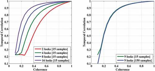
The simulation analysis shows that, for a stack of 15 interferometric pixels with NL of 9, a pixel with temporal phase correlation of 0.53, is expected to have the same phase standard deviation of a stack of 15 pixels presenting spatial phase coherence of 0.2 for the entire interferometric stack.

3. Methodology

This section describes the proposed methodology in detail. The general block diagram of the analysis steps is illustrated in Figure 3. Although our study area is the East coast of Japan, we use Sendai region throughout this section to clarify the analysis steps and demonstrates the improvements that can be achieved using the proposed analysis method.

Figure 3. Methodology block diagram.

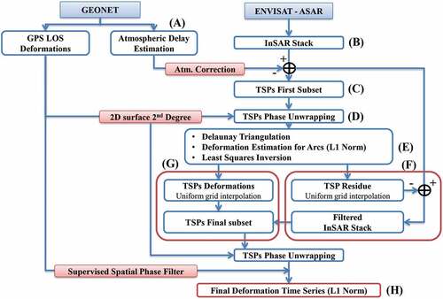
A comprehensive description of the methodology can be presented as follows. (1) We generate interferometric stack using the available SAR acquisitions. (2) We use GPS atmospheric estimation to correct for the atmospheric delay signature. (3) We identify a first subset of TSP to be used in further corrections and filtering of the InSAR stack. (4) We use GPS observations to reduce interferometric fringe rate which will facilitate the phase unwrapping process on the sparse TSPs. (5) We connect the TSPs first subset using Delaunay triangulation network and estimate the deformation for each TSP. (6) We use the residual phase of the TSPs first subset in further corrections of the InSAR stack. (7) Finally, we select all the viable pixels in the InSAR stack knowing as TSPs final subset based on the simulation results and estimate their time-variant deformations.

3.1. GPS data and atmospheric delay estimation

It is well known that the atmosphere affects microwave propagation in terms of signal delay (Hanssen 2001). The atmospheric delay is composed of three different components which are referred to as ionospheric, hydrostatic, and wet delays. The ionosphere is a region of the earth’s atmosphere extending from an altitude of about 50–1000 km where solar radiation ionizes atmospheric gases. This region contains a large number of free electrons that affect the propagating velocity of the microwave signal depending on its frequency. It has a significant effect on the L-band SAR systems, and introduce mainly planar phase artifact on the C and X-band SAR systems, that can be neglected (Meyer et al. 2006).

The hydrostatic (dry) component of the atmosphere accounts for about 90% of the tropospheric effect, this generates errors on the order of a few meters. To correct this error, several authors provided semiempirical models to achieve an estimation of the hydrostatic contribution using surface measurements such as atmospheric pressure, water vapor pressure, and temperature. Some of the most used models are Saastamoinen model (Saastamoinen 1972), Hopfield model (Hopfield 1969), and Davis model (Davis et al. 1985).

On the other hand, due to the high variation of the water vapor content, it is very difficult to model the remaining wet component. Therefore, we use raw GPS observations to estimate the Zenithal Wet Delay (ZWD) for every GPS station at the time of SAR image acquisition. For GPS processing and ZWD estimates, we use the online Automatic Precise Positioning Service (APPS) tool provided by Jet Propulsion Laboratory (JPL) of NASA (http://apps.gdgps.net/), which employs GIPSY 6.4 software.

We estimate the atmospheric (wet) component or ZWD during the position estimation of GPS stations, and because the hydrostatic models depend on stations’ altitude, the hydrostatic delay component is eliminated during the differencing process of the interferometry. This makes the wet delay component the center of focus during the atmospheric correction of the interferometric stack.

Several researchers have established the dependency of the atmospheric wet delay on the altitude (e.g. Onn and Zebker 2006). Therefore, direct application of the GPS based atmospheric correction to the interferometric stack will cause some errors, especially in areas with rough natural terrain. For that reason, we need to account for the pixels’ altitude during atmospheric correction. The adopted atmospheric correction procedure (Figure 3, Step A) can be summarized as follows: (1) We estimate the atmospheric wet delay component using GPS observations at the exact acquisition time of the SAR images. (2) We estimate the relation between ZWD and the GPS stations’ altitude for each SAR image. We assume a linear model and use least squares method to estimate its parameters using Equation (3)(3) $\mathit{ZW}{D}_{\mathit{GPS}\mathrm{stations}}=\mathit{a}\times \mathit{Altitud}{e}_{\mathit{GPS}\mathrm{stations}}+\mathit{b}\mathit{\hspace{0.17em}}$(3) . In Figure 4, we present the relation between the estimated ZWD and GPS stations’ altitude for Sendai area during the acquisition time of two SAR images. (3) We use the estimated model to calculate the ZWD at an assumed altitude of zero-meter Equation (4)(4) $\mathit{ZW}{D}_{\mathit{Zero}\mathrm{Altitude}}=\mathit{b}\mathit{\hspace{0.17em}}$(4) . (4) We use ordinary kriging interpolation method to interpolate the ZWD to a regular grid with the same dimensions of the interferograms. (5) We use DEM and the estimated model that describes the relation between ZWD and altitude to calculate the atmospheric wet delay for each pixel in the SAR image Equation (5)(5) $\mathit{ZW}{D}_{DEM\mathrm{Altitude}}^{MAP}=\mathit{ZW}{D}_{\mathrm{Zero}\mathrm{Altitude}}^{MAP}+\mathit{a}\times \mathit{Altitud}{e}_{\mathit{DEM}}\mathit{\hspace{0.17em}}$(5) . (6) For each interferogram, we calculate the atmospheric delay correction $\left(\mathit{d}\mathit{ZWD}\right)$ based on the SAR images used to generate this interferogram. Then, we multiply the estimated value by two because of the two-way passage of SAR signal through troposphere Equation (6)(6) $\begin{array}{rl}\mathit{d}\mathit{ZW}{D}_{\mathit{Interferogram}}=& 2\times \left(\mathit{ZW}{D}_{DEM\mathrm{Altitude}}^{MAP,\hspace{0.17em}Day2}\right.\\ & -\left.\mathit{ZW}{D}_{DEM\mathrm{Altitude}}^{MAP,\hspace{0.17em}Day1}\right)\end{array}$(6) . (7) We calculate the differential slant wet delay $\left(\mathit{d}\mathit{SW}{D}_i\right)$ using $\left(1/cos{\vartheta }_i\right)$ as a mapping function Equation (7)(7) $\mathit{d}\mathit{SW}{D}_i=\frac{\mathit{d}ZW{D}_i}{cos{\vartheta }_i}\mathit{\hspace{0.17em}}$(7) , where $\left({\vartheta }_i\right)$ is the incidence angle of pixel $\left(\mathit{i}\right)$. 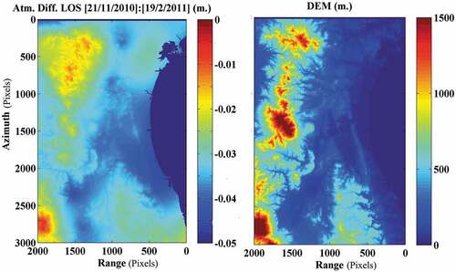In Figure 5, we present the estimated slant atmospheric (wet) delay $\left(\mathit{d}\mathit{SWD}\right)$ map for Sendai area between November 21st, 2010, and February 19th, 2011, and the DEM of the same area.

(3) $\mathit{ZW}{D}_{\mathit{GPS}\mathrm{stations}}=\mathit{a}\times \mathit{Altitud}{e}_{\mathit{GPS}\mathrm{stations}}+\mathit{b}\mathit{\hspace{0.17em}}$(3)

(4) $\mathit{ZW}{D}_{\mathit{Zero}\mathrm{Altitude}}=\mathit{b}\mathit{\hspace{0.17em}}$(4)

(5) $\mathit{ZW}{D}_{DEM\mathrm{Altitude}}^{MAP}=\mathit{ZW}{D}_{\mathrm{Zero}\mathrm{Altitude}}^{MAP}+\mathit{a}\times \mathit{Altitud}{e}_{\mathit{DEM}}\mathit{\hspace{0.17em}}$(5)

(6) $\begin{array}{rl}\mathit{d}\mathit{ZW}{D}_{\mathit{Interferogram}}=& 2\times \left(\mathit{ZW}{D}_{DEM\mathrm{Altitude}}^{MAP,\hspace{0.17em}Day2}\right.\\ & -\left.\mathit{ZW}{D}_{DEM\mathrm{Altitude}}^{MAP,\hspace{0.17em}Day1}\right)\end{array}$(6)

(7) $\mathit{d}\mathit{SW}{D}_i=\frac{\mathit{d}ZW{D}_i}{cos{\vartheta }_i}\mathit{\hspace{0.17em}}$(7)

Figure 4. Atmospheric wet delay ($\mathit{ZWD}$) vs altitude.

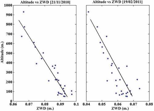
Figure 5. Atmospheric correction $\left(\mathit{d}\mathit{SWD}\right)$ and DEM.

3.2. InSAR analysis

The InSAR phase generated by two Single Look Complex (SLC) images is illustrated in Equation (8)(8) $\begin{array}{rl}& {\mathrm{\Phi }}_{\mathit{InSAR}}\\ & =\mathit{W}\left\{{\varphi }_{\mathrm{Topo}}^{Res}+{\varphi }_{\mathit{Deform}}+{\varphi }_{\mathit{Atm}}+{\varphi }_{\mathit{BL}\mathrm{Error}}+{\varphi }_{\mathit{Noise}}\right\}\end{array}$(8) , where $\mathit{W}\left\{.\right\}$ is the wrapping operator and ${\varphi }_{\mathrm{Topo}}^{Res}$ is the residual topographic component after removing the effect of topography using DEM. The InSAR phase also contains deformation ${\varphi }_{\mathit{Deform}}$, atmospheric delay ${\varphi }_{\mathit{Atm}}$, baseline error ${\varphi }_{\mathit{BL}\mathrm{Error}}$, and noise effects ${\varphi }_{\mathit{Noise}}$.

(8) $\begin{array}{rl}& {\mathrm{\Phi }}_{\mathit{InSAR}}\\ & =\mathit{W}\left\{{\varphi }_{\mathrm{Topo}}^{Res}+{\varphi }_{\mathit{Deform}}+{\varphi }_{\mathit{Atm}}+{\varphi }_{\mathit{BL}\mathrm{Error}}+{\varphi }_{\mathit{Noise}}\right\}\end{array}$(8)

After interferograms generation, flattening, and filtering (Figure 3, Step B), we apply atmospheric correction for the interferometric stack (Figure 3, Step A). Because of the interpolation process of the atmospheric delay, some of the atmospheric delay signature ${\varphi }_{Atm}^{Res}$ maybe still presented in the atmospherically corrected InSAR stack ${\mathrm{\Phi }}_{\mathrm{InSAR}}^{Atm\mathrm{Corr}}$:

(9) $\begin{array}{rl}& {\mathrm{\Phi }}_{\mathrm{InSAR}}^{Atm\mathrm{Corr}}\\ & =\mathit{W}\left\{{\varphi }_{\mathrm{Topo}}^{Res}+{\varphi }_{\mathit{Deform}}+{\varphi }_{Atm}^{Res}+{\varphi }_{\mathit{BL}\mathrm{Error}}+{\varphi }_{\mathit{Noise}}\right\}\end{array}$(9)

3.3. Temporal stable pixels

In this step, we identify the TSPs in our study area (Figure 3 Step C). As presented in Section 2.2, we define the TSPs as the pixels with temporal correlation equivalent to the expected of a pixel having a spatial coherence of 0.2, which it was found to be 0.53 at 9 look estimation window (Figure 2).

3.3.1. Identifying TSPs

Initially, we select a group of pixels based on their amplitude dispersion index, $D_{\mathrm{A}}\cong {\sigma }_{\mathrm{A}}/{\mu }_{\mathrm{A}}$ (Ferretti, Prati, and Rocca 2001), where ${\sigma }_{\mathrm{A}}$ and ${\mu }_{\mathrm{A}}$ are the standard deviation and the mean of a series of amplitude values, respectively. Because only a few SAR images are available for our area of interest, pixel selection using the amplitude dispersion index, which requires at least 30 SAR images, is ineffective. For this reason, we need to refine our selection using temporal phase stability analysis and select pixels that exhibit low phase noise, ${\varphi }_{\mathit{Noise}}$.

Recalling Equation (8)(8) $\begin{array}{rl}& {\mathrm{\Phi }}_{\mathit{InSAR}}\\ & =\mathit{W}\left\{{\varphi }_{\mathrm{Topo}}^{Res}+{\varphi }_{\mathit{Deform}}+{\varphi }_{\mathit{Atm}}+{\varphi }_{\mathit{BL}\mathrm{Error}}+{\varphi }_{\mathit{Noise}}\right\}\end{array}$(8) , the first four terms dominate the noise term, making it difficult to identify the temporal stable pixels. Therefore, to estimate the noise term ${\varphi }_{\mathit{Noise}}$, these four terms should be removed from the InSAR phase ${\mathrm{\Phi }}_{\mathit{InSAR}}$. The first four terms in Equation (8)(8) $\begin{array}{rl}& {\mathrm{\Phi }}_{\mathit{InSAR}}\\ & =\mathit{W}\left\{{\varphi }_{\mathrm{Topo}}^{Res}+{\varphi }_{\mathit{Deform}}+{\varphi }_{\mathit{Atm}}+{\varphi }_{\mathit{BL}\mathrm{Error}}+{\varphi }_{\mathit{Noise}}\right\}\end{array}$(8) are spatially correlated, except the DEM error ${\varphi }_{\mathrm{Topo}}^{Res}$ which can be partly spatially correlated.

To estimate the spatially correlated component of the phase, (Hooper, Segall, and Zebker 2007) proposed using band-pass filter as an adaptive phase filter combined with a low-pass filter in the frequency domain. It should be noted that this technique is designed to identify permanent scatterers within the interferometric pixels. In our analysis, we apply this filter to a multilooked InSAR stack, and the estimated correlation represents the combined return phase of all scatterers located within the multilooking window. A brief description of the approach is given for completeness. For a detailed description refer to (Hooper, Segall, and Zebker 2007).

(1) Pixels’ amplitudes are set to an estimate of the Signal to Noise Ratio (SNR) of the pixels, in the first iteration it is set as $1/D_{\mathrm{A}}$. (2) The complex phase is sampled to a grid to enable using 2D fast Fourier transform $\left(\mathit{FFT}\right)$, which is applied to a grid size of 32-by-32 and smoothed by a 7-by-7 pixel Gaussian window, Equation (10)(10) $\mathit{H}\left(\mathit{u},\mathit{v}\right)=\left|\mathit{Gaussian}\left(\mathit{u},\mathit{v}\right)\ast \mathit{FFT}\left[{\mathrm{\Phi }}_{\mathit{InSAR}}\right]\right|\mathit{\hspace{0.17em}}$(10) . (3) The adaptive phase filter response, $\mathit{H}\left(\mathit{u},\mathit{v}\right)$, is combined with a narrow low-pass filter response, $\mathit{L}\left(\mathit{u},\mathit{v}\right)$, to form the new filter response, $\mathit{G}\left(\mathit{u},\mathit{v}\right)$, Equation (11)(11) $\mathit{G}\left(\mathit{u},\mathit{v}\right)=\mathit{L}\left(\mathit{u},\mathit{v}\right)+0.3\left(\frac{\mathit{H}\left(\mathit{u},\mathit{v}\right)}{\bar{H}\left(\mathit{u},\mathit{v}\right)}-1\right)\mathit{\hspace{0.17em}}$(11) , (4(4) $\mathit{ZW}{D}_{\mathit{Zero}\mathrm{Altitude}}=\mathit{b}\mathit{\hspace{0.17em}}$(4) ) by applying the new filter to the resampled phase, the spatially correlated phase component,${\bar{\mathrm{\Phi }}}_{\mathit{InSAR}}$, will be obtained after 2D inverse $\mathit{FFT}$, Equation (12)(12) ${\bar{\mathrm{\Phi }}}_{\mathit{InSAR}}=\mathit{IFFT}\left[\mathit{G}\left(\mathit{u},\mathit{v}\right)\ast \mathit{FFT}\left[{\mathrm{\Phi }}_{\mathit{InSAR}}\right]\right]\mathit{\hspace{0.17em}}$(12) , where $\bar{H}\left(\mathit{u},\mathit{v}\right)$ is the median of $\mathit{H}\left(\mathit{u},\mathit{v}\right)$.

(10) $\mathit{H}\left(\mathit{u},\mathit{v}\right)=\left|\mathit{Gaussian}\left(\mathit{u},\mathit{v}\right)\ast \mathit{FFT}\left[{\mathrm{\Phi }}_{\mathit{InSAR}}\right]\right|\mathit{\hspace{0.17em}}$(10)

(11) $\mathit{G}\left(\mathit{u},\mathit{v}\right)=\mathit{L}\left(\mathit{u},\mathit{v}\right)+0.3\left(\frac{\mathit{H}\left(\mathit{u},\mathit{v}\right)}{\bar{H}\left(\mathit{u},\mathit{v}\right)}-1\right)\mathit{\hspace{0.17em}}$(11)

(12) ${\bar{\mathrm{\Phi }}}_{\mathit{InSAR}}=\mathit{IFFT}\left[\mathit{G}\left(\mathit{u},\mathit{v}\right)\ast \mathit{FFT}\left[{\mathrm{\Phi }}_{\mathit{InSAR}}\right]\right]\mathit{\hspace{0.17em}}$(12)

(5) Subtracting the filtered phase, ${\bar{\mathrm{\Phi }}}_{\mathit{InSAR}}$, from the observed phase, ${\mathrm{\Phi }}_{\mathit{InSAR}}$, and rewrapping gives an estimation of the spatially uncorrelated phase, Equation (13)(13) $\begin{array}{rl}& \mathit{W}\left\{{\mathrm{\Phi }}_{\mathit{InSAR}}-{\bar{\mathrm{\Phi }}}_{\mathit{InSAR}}\right\}\\ & =\mathit{W}\left\{{\varphi }_{\mathrm{Deform}}^u+{\varphi }_{Atm}^u+{\varphi }_{BL\mathrm{Error}}^u\right\}\\ & +\mathit{W}\left\{{\varphi }_{\mathrm{Topo}}^{Res}+{\varphi }_{\mathit{Noise}}\right\}\end{array}$(13) . The first term in the right-hand side of Equation (13)(13) $\begin{array}{rl}& \mathit{W}\left\{{\mathrm{\Phi }}_{\mathit{InSAR}}-{\bar{\mathrm{\Phi }}}_{\mathit{InSAR}}\right\}\\ & =\mathit{W}\left\{{\varphi }_{\mathrm{Deform}}^u+{\varphi }_{Atm}^u+{\varphi }_{BL\mathrm{Error}}^u\right\}\\ & +\mathit{W}\left\{{\varphi }_{\mathrm{Topo}}^{Res}+{\varphi }_{\mathit{Noise}}\right\}\end{array}$(13) is expected to be small, therefore it will be omitted. As for the second term, the effect DEM error, ${\varphi }_{\mathrm{Topo}}^{Res}$ is estimated using a periodogram, Equation (14)(14) $\begin{array}{rl}& \mathit{argma}{x}_{\mathit{\delta h}}\\ & \left\{{\gamma }_x=\left|\frac{1}{M}\sum _{\mathit{i}=1}^M{e}^{\mathit{j}\left({\mathrm{\Phi }}_{\mathit{InSAR},i}-{\bar{\mathrm{\Phi }}}_{\mathit{InSAR},\mathit{i}}\right)}.e^{-\mathit{j}\left(\frac{4\mathit{\pi }}{\lambda }\frac{{\mathit{B}}_{\mathrm{\perp i}}}{r_{i}sin{\vartheta }_i}.\mathit{\delta h}\right)}\right|\right\}\end{array}$(14) , where ${\gamma }_x$ is a measure of the phase noise level which is similar to a measure of coherence (Bamler and Just 1993), $B_{\mathrm{\perp }}$ is the perpendicular baseline, $\mathit{\lambda }$ is the signal wavelength, $\mathit{\delta h}$ is the DEM error, $r_i$ is the sensor target distance and ${\vartheta }_i$ is the incident angle, the subscript $\mathit{i}$ refers to the interferogram.

(13) $\begin{array}{rl}& \mathit{W}\left\{{\mathrm{\Phi }}_{\mathit{InSAR}}-{\bar{\mathrm{\Phi }}}_{\mathit{InSAR}}\right\}\\ & =\mathit{W}\left\{{\varphi }_{\mathrm{Deform}}^u+{\varphi }_{Atm}^u+{\varphi }_{BL\mathrm{Error}}^u\right\}\\ & +\mathit{W}\left\{{\varphi }_{\mathrm{Topo}}^{Res}+{\varphi }_{\mathit{Noise}}\right\}\end{array}$(13)

(14) $\begin{array}{rl}& \mathit{argma}{x}_{\mathit{\delta h}}\\ & \left\{{\gamma }_x=\left|\frac{1}{M}\sum _{\mathit{i}=1}^M{e}^{\mathit{j}\left({\mathrm{\Phi }}_{\mathit{InSAR},i}-{\bar{\mathrm{\Phi }}}_{\mathit{InSAR},\mathit{i}}\right)}.e^{-\mathit{j}\left(\frac{4\mathit{\pi }}{\lambda }\frac{{\mathit{B}}_{\mathrm{\perp i}}}{r_{i}sin{\vartheta }_i}.\mathit{\delta h}\right)}\right|\right\}\end{array}$(14)

(6) Subtracting the DEM error, ${\hat{\varphi }}_{\mathit{Topo}}^{\mathit{Res}}$, from Equation (13)(13) $\begin{array}{rl}& \mathit{W}\left\{{\mathrm{\Phi }}_{\mathit{InSAR}}-{\bar{\mathrm{\Phi }}}_{\mathit{InSAR}}\right\}\\ & =\mathit{W}\left\{{\varphi }_{\mathrm{Deform}}^u+{\varphi }_{Atm}^u+{\varphi }_{BL\mathrm{Error}}^u\right\}\\ & +\mathit{W}\left\{{\varphi }_{\mathrm{Topo}}^{Res}+{\varphi }_{\mathit{Noise}}\right\}\end{array}$(13) , makes Equation (15)(15) $\mathit{W}\left\{{\mathrm{\Phi }}_{\mathit{InSAR}}-{\bar{\mathrm{\Phi }}}_{\mathit{InSAR}}-{\hat{\varphi }}_{\mathit{Topo}}^{\mathit{Res}}\right\}=\mathit{W}\left\{{\hat{\varphi }}_{\mathit{Noise}}\right\}\mathit{\hspace{0.17em}}$(15) the first estimation of the pixel’s noise ${\hat{\varphi }}_{\mathit{Noise}}$.

(15) $\mathit{W}\left\{{\mathrm{\Phi }}_{\mathit{InSAR}}-{\bar{\mathrm{\Phi }}}_{\mathit{InSAR}}-{\hat{\varphi }}_{\mathit{Topo}}^{\mathit{Res}}\right\}=\mathit{W}\left\{{\hat{\varphi }}_{\mathit{Noise}}\right\}\mathit{\hspace{0.17em}}$(15)

(7) Calculate the SNR for every pixel using phase noise ${\hat{\varphi }}_{\mathit{Noise}}$, Equation (16)(16.a) $\mathit{SNR}=\frac{g^2}{2{\sigma }_n^2}\mathit{\hspace{0.17em}}$(16.a) .

(16.a) $\mathit{SNR}=\frac{g^2}{2{\sigma }_n^2}\mathit{\hspace{0.17em}}$(16.a)

(16.b) $\hat{g}=\frac{1}{N}\sum _{\mathit{i}=1}^N{A}_{i}cos{\hat{\varphi }}_{\mathit{Noise},\mathit{i}}\mathit{\hspace{0.17em}}$(16.b)

(16.c) ${\hat{\sigma }}_{\mathit{n}}^2=\frac{1}{2}\left[\frac{{\sum }_{i=1}^N{A}_i^2}{\mathit{N}}-{\hat{g}}^2\right]\mathit{\hspace{0.17em}}$(16.c)

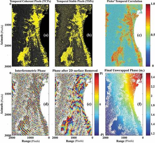
where $\mathit{g}$ is the signal amplitude, $\mathit{A}$ is the observed amplitude and ${\hat{\sigma }}_{\mathit{n}}^2$ is the noise variance. (8) The process is repeated using the estimated SNR as a weight factor. The system converges when ${\gamma }_x$ cease of decreasing. In Figure 6(c) we present the temporal correlation map of Sendai area. It is clear that in urban regions the phase temporal correlation is high, whereas in vegetated regions it is very low, which is the expected behavior.

Figure 6. Analysis of Sendai region (a) TCPs, (b) TSPs first subset. (c) Phase temporal correlation. (d) Coseismic interferogram before applying GPS fringe reduction and (e) after, (f) the corresponding final unwrapped phase map.

3.3.2. TSPs first subset

In this step, we select a first TSPs subset of the most reliable pixels to be used in phase filtering by setting a threshold to the final estimation of ${\gamma }_x\ge 0.7$. We use this subset to determine the remaining imposed nuisance phase to the InSAR stack. This process facilitates finer phase refinement which assists in estimating accurate deformations with high spatial coverage in the presence of rough and vegetated surface signature.

Figure 6(a,b) present a comparison between the first TSPs subset (${\gamma }_x\ge 0.7$) in Sendai region, and the pixels present a spatial phase coherence of $\ge 0.2$ for the entire InSAR stack. The number of identified pixels, pixels density, and coverage index of each group is presented in Table 2. The data show that the number of TCPs (727,763 pixels) is larger than the first TSP subset (173,282 pixels), which makes the TCP pixels density (169.7 pixels/km²) much better than the TSP pixels density (40.4 pixels/km²). But these parameters can be deceiving regarding the amount of area being covered in the analysis, mainly because the identified TCPs can be clustered in few regions with large numbers, which excludes vast areas from being covered in the analysis (Figure 6(a).

Table 2. Pixels density and coverage index

Region	Pixel type	No. of pixels	Density (Pixel/km^2)	Coverage Index	Change rate (%)
Aomori	TCP	271,095	53.3	0.37	+ 61
	TSP (first subset)	87,561	17.2	0.98
Iwate	TCP	452,545	58.0	0.40	+ 59
	TSP (first subset)	136,117	17.4	0.99
Sendai	TCP	727,763	169.7	0.60	+ 39
	TSP (first subset)	173,211	40.4	0.99
Iwaki	TCP	1,739,378	134.3	0.75	+ 23
	TSP (first subset)	289,035	36.8	0.98
Chiba	TCP	1,954,660	440.8	0.98	+ 2
	TSP (first subset)	465,854	105.1	1.00
Mean					+ 36.8

To get a better estimation of the covered area, we calculate the coverage index of each group of pixels. First, we use Delaunay triangulation network to connect all the pixels in each group with a maximum arc length of 3000 m. The coverage index is the ratio between the planer areas of Delaunay triangles to the land area included in the image Equation (17)(17) $\mathit{Coverage}\mathit{Index}=\mathit{\hspace{0.17em}}\frac{{\sum }_{i=1}^{no.\mathrm{Triangles}}\mathit{Area}\mathit{of}\mathit{Triangle},\mathit{i}}{\mathit{Total}\mathit{Land}\mathit{Area}}$(17) , which ranges between zero for no coverage and one for total coverage.

(17) $\mathit{Coverage}\mathit{Index}=\mathit{\hspace{0.17em}}\frac{{\sum }_{i=1}^{no.\mathrm{Triangles}}\mathit{Area}\mathit{of}\mathit{Triangle},\mathit{i}}{\mathit{Total}\mathit{Land}\mathit{Area}}$(17)

We find the value of the coverage index for the TSPs is 0.99 while it is 0.6 for the TCPs. This means that the spatial distribution of the TSPs’ first subset increases the spatial coverage of the study area and improves the interferometric correction process.

After selecting TSPs first subset, we correct their atmospheric corrected phase, Equation (9)(9) $\begin{array}{rl}& {\mathrm{\Phi }}_{\mathrm{InSAR}}^{Atm\mathrm{Corr}}\\ & =\mathit{W}\left\{{\varphi }_{\mathrm{Topo}}^{Res}+{\varphi }_{\mathit{Deform}}+{\varphi }_{Atm}^{Res}+{\varphi }_{\mathit{BL}\mathrm{Error}}+{\varphi }_{\mathit{Noise}}\right\}\end{array}$(9) , for DEM error ${\varphi }_{\mathrm{Topo}}^{Res}$ estimated by Equation (14)(14) $\begin{array}{rl}& \mathit{argma}{x}_{\mathit{\delta h}}\\ & \left\{{\gamma }_x=\left|\frac{1}{M}\sum _{\mathit{i}=1}^M{e}^{\mathit{j}\left({\mathrm{\Phi }}_{\mathit{InSAR},i}-{\bar{\mathrm{\Phi }}}_{\mathit{InSAR},\mathit{i}}\right)}.e^{-\mathit{j}\left(\frac{4\mathit{\pi }}{\lambda }\frac{{\mathit{B}}_{\mathrm{\perp i}}}{r_{i}sin{\vartheta }_i}.\mathit{\delta h}\right)}\right|\right\}\end{array}$(14) , the atmospheric and topographic corrected phase is presented as

(18) $\begin{array}{rl}& {\mathrm{\Phi }}_{\mathrm{TSPs}}^{Atm\mathrm{Topo}\mathrm{Corr}.}\\ & =\mathit{W}\left\{{\varphi }_{\mathit{Deform}}+{\varphi }_{Atm}^{Res}+{\varphi }_{\mathit{BL}\mathrm{Error}}+{\varphi }_{\mathit{Noise}}\right\}\end{array}$(18)

3.4. Temporal stable pixels phase unwrapping

For the phase unwrapping process of TSPs, we use Delaney Minimum Cost Flow (DMCF) (Costantini and Rosen 1999) method. When studying major shock earthquakes, using any phase unwrapping method on sparse pixels can be a very challenging process, especially in C and X-Band SAR systems. This intensifies the rate of the interferometric fringes, which reduces the reliability of the phase unwrapping process.

Therefore, we suggest using the GPS observation to reduce the fringe rate of the interferograms, which will increase the success rate and reliability of the phase unwrapping results. We use the Line-Of-Sight (LOS) GPS observation to model a 2D surface of the second degree. Then subtract this 2D surface from the interferograms before the phase unwrapping process, and restore it to the unwrapped phase maps (Figure 3, Step D). It is not intended to model the full deformation signature of the earthquake, just the long-wave effect to reduce the interferometric fringe rate.

In Figure 6, we present the coseismic interferogram of Sendai area before and after subtracting the 2D surface. The fringe rate is reduced significantly, which increases the probability of a successful phase unwrapping over a sparse grid. In addition, we present the unwrapped phase map after restoring the 2D surface.

3.5. Estimating deformation for first TSPs subset

We use the unwrapped phase difference between neighboring pixels as the basic observation for the deformation estimation of TSPs’ first subset (Figure 3, Step E). This technique reduces the effect of the spatially correlated errors which was proven to be efficient by several researchers (e.g. Ferretti, Prati, and Rocca 2000; Mora, Mallorqui, and Broquetas 2003; Liu et al. 2009; Zhang et al. 2014).

We connect all TSPs in an interferogram using Delaunay triangulation network each connection is called an arc. We use a maximum 3D arc length of 3000 m. Although it is common to set an arc length threshold of 1000 m, we decided to liberate this threshold because the InSAR phase has been corrected for the atmospheric delay. Extending the arc length threshold improves the connection between the TSPs, especially in the areas with varying altitudes.

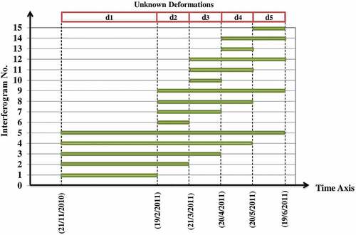
Let the number of SAR images for the area of interest is $\mathit{N}$ and ordered in a time series $\left(t_1:t_N\right)$, number of unknown deformations for each pixel equals $\left(\mathit{n}=\mathit{N}-1\right)$ and identified by $\left(d_1:d_n\right)$, which is shown in Figure 7. In addition, let the number of differential interferograms is $\mathit{M}$, number of arcs is $\mathit{S}$, number of TSPs is $\mathit{K}$, and the phase difference between two TSPs, $\mathrm{\Delta }{\varphi }_{a,b}^{,i}$, in the $i^{\mathit{th}}$ unwrapped phase map, Equation (19)(19) $\mathrm{\Delta }{\varphi }_{a,b}^{Atm\mathrm{Topo}\mathrm{Corr},i}=\mathrm{\Delta }{\varphi }_{\mathrm{Deform},\hspace{0.17em}a,b}^i+\mathrm{\Delta }{\varphi }_{Atm,\hspace{0.17em}a,b}^{Res,i}+\mathrm{\Delta }{\varphi }_{BL\mathrm{Error},\hspace{0.17em}a,b}^i+\mathrm{\Delta }{\varphi }_{\mathrm{Noise},\hspace{0.17em}a,b}^i\mathit{\hspace{0.17em}},\mathit{\hspace{0.17em}}\mathit{i}=1:\mathit{M}$(19) . For neighboring pixels, the spatially correlated errors, $\mathrm{\Delta }{\varphi }_{Atm,\hspace{0.17em}a,b}^{Res,i}$ and $\mathrm{\Delta }{\varphi }_{BL\mathrm{Error},\hspace{0.17em}a,b}^i$ are significantly reduced.

(19) $\mathrm{\Delta }{\varphi }_{a,b}^{Atm\mathrm{Topo}\mathrm{Corr},i}=\mathrm{\Delta }{\varphi }_{\mathrm{Deform},\hspace{0.17em}a,b}^i+\mathrm{\Delta }{\varphi }_{Atm,\hspace{0.17em}a,b}^{Res,i}+\mathrm{\Delta }{\varphi }_{BL\mathrm{Error},\hspace{0.17em}a,b}^i+\mathrm{\Delta }{\varphi }_{\mathrm{Noise},\hspace{0.17em}a,b}^i\mathit{\hspace{0.17em}},\mathit{\hspace{0.17em}}\mathit{i}=1:\mathit{M}$(19)

Figure 7. InSAR stack structure.

For each arc, we use L1-norm to solve for the unknown deformation velocities $\mathrm{\Delta }\mathit{V}$ by minimizing the error function E, Equation (20.a)(20.a) $\mathit{E}=\mathit{argmin}\sum _{\mathit{i}=1}^M\left|\mathrm{\Delta }{\varphi }_j^{Atm\mathrm{Topo}\mathrm{Corr},i}-\mathit{B}\mathrm{\Delta }{\mathit{V}}_j\right|\mathit{\hspace{0.17em}},\mathit{j}=1:\mathit{S}\mathit{\hspace{0.17em}}$(20.a) , (Lauknes, Zebker, and Larsen 2011), where $\mathit{B}$ is the design matrix of the system, which is the partial derivatives of deformation represented by each interferogram $D_i$ with respect to the velocity in each time segment for an arc $\left[\mathrm{\Delta }{V}_1:\mathrm{\Delta }{V}_n\right]$. The deformation equation of interferogram No. 8, Figure 7 is presented in Equation (20.b)(20.b) $D_8={\left[\left(\mathrm{\Delta }{t}_2.\mathrm{\Delta }{V}_2\right)+\left(\mathrm{\Delta }{t}_3.\mathrm{\Delta }{V}_3\right)+\left(\mathrm{\Delta }{t}_4.\mathrm{\Delta }{V}_4\right)\right]}_{\mathit{j}}\mathit{\hspace{0.17em}}$(20.b) as an illustrative example.

The difference between L1-norm and L2-norm is that the L1-norm minimizes the sum of residuals magnitudes, while the L2-norm minimizes the sum of squared residuals magnitudes. Consequently, the L1-norm does not square each term of the misfit, resulting in a solution that is more robust to outliers (Huber 1987).

(20.a) $\mathit{E}=\mathit{argmin}\sum _{\mathit{i}=1}^M\left|\mathrm{\Delta }{\varphi }_j^{Atm\mathrm{Topo}\mathrm{Corr},i}-\mathit{B}\mathrm{\Delta }{\mathit{V}}_j\right|\mathit{\hspace{0.17em}},\mathit{j}=1:\mathit{S}\mathit{\hspace{0.17em}}$(20.a)

(20.b) $D_8={\left[\left(\mathrm{\Delta }{t}_2.\mathrm{\Delta }{V}_2\right)+\left(\mathrm{\Delta }{t}_3.\mathrm{\Delta }{V}_3\right)+\left(\mathrm{\Delta }{t}_4.\mathrm{\Delta }{V}_4\right)\right]}_{\mathit{j}}\mathit{\hspace{0.17em}}$(20.b)

where

$\mathit{B}={\left[\begin{array}{ccc}\frac{\mathrm{\partial }{D}_1}{\mathrm{\partial \Delta }{V}_1}& \cdots & \frac{\mathrm{\partial }{D}_1}{\mathrm{\partial \Delta }{V}_n}\\ ⋮& \ddots & ⋮\\ \frac{\mathrm{\partial }{D}_M}{\mathrm{\partial \Delta }{V}_1}& \cdots & \frac{\mathrm{\partial }{D}_M}{\mathrm{\partial \Delta }{V}_n}\end{array}\right]}_{\mathit{M}\times \mathit{n}};\mathrm{\Delta }{\mathit{V}}_j=\left[\begin{array}{c}\mathrm{\Delta }{V}_{\mathit{j},1}\\ ⋮\\ \mathrm{\Delta }{V}_{\mathit{j},\mathit{n}}\end{array}\right]$

For solving the L1-norm optimization problem, we use the method proposed by (Schlossmacher 1973). The method is based on an iterative solution of a weighted ordinary least squares problem. The principle behind the iteratively reweighted least squares method is that the weight matrix is adjusted corresponding to the current residuals at each iteration, which de-emphasizes observations with large residuals. The iterations terminate when residuals cease from changing between successive iterations.

Assuming a full-rank of the design matrix $\mathit{B}$, the iterating system follows Equation (21.a)(20.a) $\mathit{E}=\mathit{argmin}\sum _{\mathit{i}=1}^M\left|\mathrm{\Delta }{\varphi }_j^{Atm\mathrm{Topo}\mathrm{Corr},i}-\mathit{B}\mathrm{\Delta }{\mathit{V}}_j\right|\mathit{\hspace{0.17em}},\mathit{j}=1:\mathit{S}\mathit{\hspace{0.17em}}$(20.a) , where $\mathit{W}\left(\mathit{k}\right)$ is the diagonal weighting matrix at the $k^{\mathit{th}}$ iteration, which is inversely proportional to the absolute residuals estimated from the previous iteration $\left(\mathit{k}-1\right)$ (see Equation (21.b)(20.b) $D_8={\left[\left(\mathrm{\Delta }{t}_2.\mathrm{\Delta }{V}_2\right)+\left(\mathrm{\Delta }{t}_3.\mathrm{\Delta }{V}_3\right)+\left(\mathrm{\Delta }{t}_4.\mathrm{\Delta }{V}_4\right)\right]}_{\mathit{j}}\mathit{\hspace{0.17em}}$(20.b) . In the first iteration, the weights are chosen to be unity.

(21.a) $\left({\mathit{B}}^{\mathrm{T}}\mathit{W}\left(\mathit{k}\right)\mathit{B}\right).\mathrm{\Delta }\mathit{V}\left(\mathit{k}\right)=\mathit{\hspace{0.17em}}{\mathit{B}}^{\mathrm{T}}\mathit{W}\left(\mathit{k}\right)\mathrm{\Delta }{\varphi }_j^{Atm\mathrm{Topo}\mathrm{Corr}}$(21.a)

(21.b) $\mathit{W}\left(\mathit{k}\right)={\left[\begin{array}{ccc}{\left|\mathrm{\Delta }{\varphi }_j^{Atm\mathrm{Topo}\mathrm{Corr}}-\mathit{B}.\mathrm{\Delta }{\mathit{V}}_{\mathit{j}}\left(\mathit{k}-1\right)\right|}_1^{-1}& 0& 0\\ 0& \ddots & 0\\ 0& 0& {\left|\mathrm{\Delta }{\varphi }_j^{Atm\mathrm{Topo}\mathrm{Corr}}-\mathit{B}.\mathrm{\Delta }{\mathit{V}}_{\mathit{j}}\left(\mathit{k}-1\right)\right|}_{\mathit{M}}^{-1}\end{array}\right]}_{\mathit{M}\times \mathit{M}}$(21.b)

Finally, the deformation velocity values for each TSP can be estimated using least squares inversion, Equation (22)(22) $\mathit{L}=\mathit{A}.\mathit{V}$(22) , this inversion is applied to every time segment, i.e. $\mathit{n}$ times. Here, $\left[\mathit{A}\right]$ is the design matrix relating the arcs, $\left(\mathit{S}\right)$, with the TSP pixels $\left(\mathit{K}\right)$, $\left[\mathit{L}\right]$ contains the estimated velocities for all the arcs in a certain time segment $\mathit{q}$ and $\left[\mathit{V}\right]$ is the unknown velocity vector for the TSPs. It should be noted that Equation (22)(22) $\mathit{L}=\mathit{A}.\mathit{V}$(22) is a large sparse linear system that can be solved by an iterative method based on a bidiagonalization procedure that appears in Matlab as a built-in LSQR function (Paige and Saunders 1982).

(22) $\mathit{L}=\mathit{A}.\mathit{V}$(22)

where

$\begin{array}{rl}& \mathit{A}={\left[\begin{array}{ccc}1& 0& \cdots \\ 1& -1& \cdots \\ ⋮& ⋮& \ddots \end{array}\right]}_{\mathit{S}\times \mathit{K}},\mathit{\hspace{0.17em}}\mathit{L}=\left[\begin{array}{c}\mathrm{\Delta }{V}_{1,\mathit{q}}\\ ⋮\\ \mathrm{\Delta }{V}_{\mathit{S},\mathit{q}}\end{array}\right],\mathit{\hspace{0.17em}}\\ & \mathit{V}=\left[\begin{array}{c}{V}_{1,\mathit{q}}\\ ⋮\\ V_{\mathit{K},\mathit{q}}\end{array}\right],\mathrm{and}\mathit{q}=\left[1:\mathit{n}\right]\end{array}$

3.6. Filtering interferograms

After estimating the time-variant velocity of each TSP, $\left[\mathbf{V}\right]$, Equation (22)(22) $\mathit{L}=\mathit{A}.\mathit{V}$(22) , we can assume that most of the atmospheric delay, baseline error, and phase noise were eliminated or significantly reduced. These imposed errors are spatially correlated except phase noise ${\varphi }_{\mathit{Noise}}$. Therefore, we propose estimating the phase errors for each interferogram at the TSPs locations, which have high spatial coverage and interpolate them to a regular grid, which will be used in further filtering of the InSAR stack (Figure 3, Step F).

First, we calculate the corrected phase of the TSPs first subset,${\varphi }_{\mathrm{TSPs}}^{\mathrm{Corrected}}$, for each interferogram of the stack using Equation (23)(23) ${\varphi }_{\mathrm{TSPs}}^{\mathrm{Corrected}}=\mathit{B}.\mathit{V}\mathit{\hspace{0.17em}}$(23) , where $\left[\mathit{B}\right]$ is the design matrix relating the interferograms with the time-variant velocities of arc observations $\left[\mathrm{\Delta }\mathit{V}\right]$, Equation (20)(20.a) $\mathit{E}=\mathit{argmin}\sum _{\mathit{i}=1}^M\left|\mathrm{\Delta }{\varphi }_j^{Atm\mathrm{Topo}\mathrm{Corr},i}-\mathit{B}\mathrm{\Delta }{\mathit{V}}_j\right|\mathit{\hspace{0.17em}},\mathit{j}=1:\mathit{S}\mathit{\hspace{0.17em}}$(20.a) , and can be used to relate the same interferograms to the TSPs time-variant velocities without any change. Then, we calculate the TSPs phase residues,${\varphi }_{\mathrm{TSPs}}^{\mathrm{Residue}}$, Equation (24)(24) ${\varphi }_{\mathrm{TSPs}}^{\mathrm{Residue}}={\varphi }_{\mathrm{TSPs}}^{Atm\mathrm{Topo}\mathrm{Corr}.}-{\varphi }_{\mathrm{TSPs}}^{\mathrm{Corrected}}={\varphi }_{Atm,\hspace{0.17em}\mathrm{TSPs}}^{Res}+{\varphi }_{BL\mathrm{Error},\hspace{0.17em}\mathrm{TSPs}}^{\hspace{0.17em}}+{\varphi }_{\mathrm{Noise}}^{\hspace{0.17em}}\mathit{\hspace{0.17em}}$(24) by subtracting Equation (18)(18) $\begin{array}{rl}& {\mathrm{\Phi }}_{\mathrm{TSPs}}^{Atm\mathrm{Topo}\mathrm{Corr}.}\\ & =\mathit{W}\left\{{\varphi }_{\mathit{Deform}}+{\varphi }_{Atm}^{Res}+{\varphi }_{\mathit{BL}\mathrm{Error}}+{\varphi }_{\mathit{Noise}}\right\}\end{array}$(18) , after phase unwrapping, and Equation (23)(23) ${\varphi }_{\mathrm{TSPs}}^{\mathrm{Corrected}}=\mathit{B}.\mathit{V}\mathit{\hspace{0.17em}}$(23) . Finally, we interpolate phase residues to a regular grid and subtract it from its corresponding interferogram, Equation (9)(9) $\begin{array}{rl}& {\mathrm{\Phi }}_{\mathrm{InSAR}}^{Atm\mathrm{Corr}}\\ & =\mathit{W}\left\{{\varphi }_{\mathrm{Topo}}^{Res}+{\varphi }_{\mathit{Deform}}+{\varphi }_{Atm}^{Res}+{\varphi }_{\mathit{BL}\mathrm{Error}}+{\varphi }_{\mathit{Noise}}\right\}\end{array}$(9) , and rewrapping. This process results in a filtered estimation of the InSAR phase, ${\mathrm{\Phi }}_{\mathrm{InSAR}}^{\mathrm{Filtered}}$, Equation (25)(25) ${\mathrm{\Phi }}_{\mathrm{InSAR}}^{\mathrm{Filtered}}=\mathit{W}\left\{{\varphi }_{\mathrm{Topo}}^{Res}+{\varphi }_{\mathit{Deform}}+{\varphi }_{\mathit{Noise}}\right\}\mathit{\hspace{0.17em}}$(25) .

(23) ${\varphi }_{\mathrm{TSPs}}^{\mathrm{Corrected}}=\mathit{B}.\mathit{V}\mathit{\hspace{0.17em}}$(23)

(24) ${\varphi }_{\mathrm{TSPs}}^{\mathrm{Residue}}={\varphi }_{\mathrm{TSPs}}^{Atm\mathrm{Topo}\mathrm{Corr}.}-{\varphi }_{\mathrm{TSPs}}^{\mathrm{Corrected}}={\varphi }_{Atm,\hspace{0.17em}\mathrm{TSPs}}^{Res}+{\varphi }_{BL\mathrm{Error},\hspace{0.17em}\mathrm{TSPs}}^{\hspace{0.17em}}+{\varphi }_{\mathrm{Noise}}^{\hspace{0.17em}}\mathit{\hspace{0.17em}}$(24)

(25) ${\mathrm{\Phi }}_{\mathrm{InSAR}}^{\mathrm{Filtered}}=\mathit{W}\left\{{\varphi }_{\mathrm{Topo}}^{Res}+{\varphi }_{\mathit{Deform}}+{\varphi }_{\mathit{Noise}}\right\}\mathit{\hspace{0.17em}}$(25)

3.7. Final temporal stable pixels deformation maps

For the first TSPs subset, we use a temporal correlation threshold of ${\gamma }_x\ge 0.7$ (Equation (14)(14) $\begin{array}{rl}& \mathit{argma}{x}_{\mathit{\delta h}}\\ & \left\{{\gamma }_x=\left|\frac{1}{M}\sum _{\mathit{i}=1}^M{e}^{\mathit{j}\left({\mathrm{\Phi }}_{\mathit{InSAR},i}-{\bar{\mathrm{\Phi }}}_{\mathit{InSAR},\mathit{i}}\right)}.e^{-\mathit{j}\left(\frac{4\mathit{\pi }}{\lambda }\frac{{\mathit{B}}_{\mathrm{\perp i}}}{r_{i}sin{\vartheta }_i}.\mathit{\delta h}\right)}\right|\right\}\end{array}$(14) . The number of selected TSPs is remarkably smaller than that of TCP nearly one-fourth (Figure 6). This means that there are many reliable pixels that we neglected in the first TSPs subset. However, the first TSPs subset is adequate for correcting the InSAR stack, taking into consideration its high phase reliability and spatial coverage.

In this step, we identify all reliable pixels within the InSAR stack to increase the analysis covered area (Figure 3, Step G). Therefore, we select the pixels with a temporal correlation of ${\gamma }_x\ge 0.53$, which is based on the simulation analysis in Section 2.2. We use the same temporal correlation maps generated when selecting the TSPs’ first subset, e.g. Figure 6(c), because the illustrated filtering process does not affect the pixels’ phase noise.

The number of pixels identified as TSPs final subset in Sendai region is (968,678 pixels), which makes the TSPs density (225.86 pixels/km²) much better than the TCPs density (169.7 pixels/km²). Moreover, the number of pixels identified as reliable TSPs and rejected in TCPs technique because they present spatial coherence less than 0.2 is (240,915 pixels). This means, using TSPs techniques increases the number of reliable pixels identified in Sendai region by 33.1%, (Table 3).

Table 3. Number of temporal stable pixels final subset

Region	TSPs (final subset)	TSPs with coherence < 0.2	Change rate vs TCP (%)
Aomori	428,768	157,673	58.2
Iwate	772,483	319,938	70.7
Sendai	968,678	240,915	33.1
Iwaki	1,739,378	685,665	65.1
Chiba	2,438,949	484,289	24.8
Mean			50.38

The phase of the final TSPs is presented in Equation (25)(25) ${\mathrm{\Phi }}_{\mathrm{InSAR}}^{\mathrm{Filtered}}=\mathit{W}\left\{{\varphi }_{\mathrm{Topo}}^{Res}+{\varphi }_{\mathit{Deform}}+{\varphi }_{\mathit{Noise}}\right\}\mathit{\hspace{0.17em}}$(25) . It contains residual topographic phase, deformation phase, and phase noise. The main interest is to isolate the deformation phase ${\varphi }_{\mathit{Deform}}$, and correct for the other components. To estimate the topographic and deformation phases, a periodogram in these two components can be used as proposed by (Ferretti, Prati, and Rocca 2001). Unfortunately, this process is not adequate for large areas and can be computationally intensive. Therefore, we propose interpolating the corrected deformations estimated by the TSPs first subset,${\varphi }_{\mathrm{TSPs}}^{\mathrm{Corrected}}$, to a regular grid, ${\varphi }_{\mathrm{TSPs},\hspace{0.17em}Map}^{\mathrm{Corrected}}$, and subtract it from the filtered InSAR stack, ${\mathrm{\Phi }}_{\mathrm{InSAR}}^{\mathrm{Filtered}}$, which reduces the deformation signature significantly, Equation (26)(26) ${\varphi }_{\mathrm{InSAR}}^{\mathrm{Residuals}}=\mathit{W}\left\{{\mathrm{\Phi }}_{\mathrm{InSAR}}^{\mathrm{Filtered}}-{\varphi }_{\mathrm{TSPs},\hspace{0.17em}Map}^{\mathrm{Corrected}}\right\}=\mathit{W}\left\{{\varphi }_{\mathrm{Topo}}^{Res}+{\varphi }_{\mathrm{Deform}}^{Res}+{\varphi }_{\mathit{Noise}}\right\}\mathit{\hspace{0.17em}}$(26) . Then, we can use a simple periodogram, Equation (14)(14) $\begin{array}{rl}& \mathit{argma}{x}_{\mathit{\delta h}}\\ & \left\{{\gamma }_x=\left|\frac{1}{M}\sum _{\mathit{i}=1}^M{e}^{\mathit{j}\left({\mathrm{\Phi }}_{\mathit{InSAR},i}-{\bar{\mathrm{\Phi }}}_{\mathit{InSAR},\mathit{i}}\right)}.e^{-\mathit{j}\left(\frac{4\mathit{\pi }}{\lambda }\frac{{\mathit{B}}_{\mathrm{\perp i}}}{r_{i}sin{\vartheta }_i}.\mathit{\delta h}\right)}\right|\right\}\end{array}$(14) , to estimate and correct for the residual topographic phase,${\varphi }_{\mathrm{Topo}}^{Res}$, Equation (27)(27) ${\mathrm{\Phi }}_{\mathrm{Final}\mathrm{TSPs}}^{\mathrm{Filtered}}=\mathit{W}\left\{{\varphi }_{\mathit{Deform}}+{\varphi }_{\mathit{Noise}}\right\}\mathit{\hspace{0.17em}}$(27) .

(26) ${\varphi }_{\mathrm{InSAR}}^{\mathrm{Residuals}}=\mathit{W}\left\{{\mathrm{\Phi }}_{\mathrm{InSAR}}^{\mathrm{Filtered}}-{\varphi }_{\mathrm{TSPs},\hspace{0.17em}Map}^{\mathrm{Corrected}}\right\}=\mathit{W}\left\{{\varphi }_{\mathrm{Topo}}^{Res}+{\varphi }_{\mathrm{Deform}}^{Res}+{\varphi }_{\mathit{Noise}}\right\}\mathit{\hspace{0.17em}}$(26)

(27) ${\mathrm{\Phi }}_{\mathrm{Final}\mathrm{TSPs}}^{\mathrm{Filtered}}=\mathit{W}\left\{{\varphi }_{\mathit{Deform}}+{\varphi }_{\mathit{Noise}}\right\}\mathit{\hspace{0.17em}}$(27)

After that, we apply the phase unwrapping to the final TSPs subset using DMCF and GPS observations, as described in Section 3.4 (Figure 3, Step D). Then, we apply a GPS-based supervised spatial phase filter (ElGharbawi and Tamura 2014a) to remove any residual spatial component of the baseline error that may be presented in the InSAR stack. The idea of this filter is to estimate the phase error at the locations of GPS stations by subtracting the GPS observed LOS deformations from its corresponding filtered InSAR phase. Then, these errors are used to model a 2D surface and remove it from the unwrapped phase maps. We use the GPS-based spatial filter because the deformation signature of the 2011 Tohoku earthquake dominates the entire interferograms, and a simple phase ramp removal will affect the deformation signature of the earthquake.

Finally, we estimate the time-variant deformations of the final TSPs subset using the L1-norm, as described in Section 3.5, Equation (20)(20.a) $\mathit{E}=\mathit{argmin}\sum _{\mathit{i}=1}^M\left|\mathrm{\Delta }{\varphi }_j^{Atm\mathrm{Topo}\mathrm{Corr},i}-\mathit{B}\mathrm{\Delta }{\mathit{V}}_j\right|\mathit{\hspace{0.17em}},\mathit{j}=1:\mathit{S}\mathit{\hspace{0.17em}}$(20.a) . The final deformation estimation is applied to each pixel (Figure 3, Step H), not employing arcs, which reduces the computational load significantly.

4. Application to the East coast of Japan

4.1. Data preparation

We use six C-band Single polarization (HH) SAR images for northeastern Japan, which were acquired by ENVISAT ASAR in descending direction (Table 1). The data were provided by the European Space Agency © ESA (2014). We generate the InSAR stack as shown in Figure 7 and Table 1 and remove the topography effect using SRTM 3 DEM. We use Goldstein method (Goldstein and Werner 1998) for filtering and Delaney Minimum Cost Flow DMCF (Costantini and Rosen 1999) method for phase unwrapping. To reduce phase decorrelation, we use a multi looking of 3-by-9 looks in the range and azimuth directions, respectively.

4.2. Steps of analysis

We subdivided the analysis area into several regions and analyzed each region separately to reduce the computational load. For each region, we follow the steps of the methodology described in Section 3. First, we generate the InSAR stack as shown in Figure 7 (Figure 3, Step B). Then, we estimate the atmospheric ZWD using GPS observations at the exact acquisition time of every SAR image. Then, we use kriging interpolation and DEM to estimate the atmospheric correction map for each interferogram (Figure 3, Step A). After correcting every interferogram for the atmospheric delay, we select the first TSPs subset. Initially, we use an amplitude dispersion index of $D_{\mathrm{A}}\le 0.4$, then we refine the selection using temporal phase stability analysis and set the temporal correlation threshold to ${\gamma }_x\ge 0.7$ (Figure 3, Step C).

In Figure 8, we present a comparison between the TCP and the first TSPs subsets in Aomori, Iwate, Iwaki, and Chiba regions. The spatial coverage of TSPs is much better than the spatial coverage of TCPs. In Chiba, the spatial coverage of TCPs and TSPs is very comparable, mainly because Chiba region contains many urban areas and has low vegetation coverage.

Figure 8. TCPs and TSPs first subset in Aomori, Iwate, Iwaki, and Chiba regions.

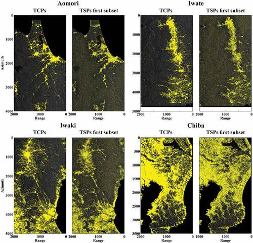
For better illustration, we present in Table 2 the number of pixels, pixel density, and coverage index for the TCPs and the first subset of TSPs. The number of pixels and pixel density for TCPs is much higher than the TSPs’ first subset. On the other hand, the coverage index of TSPs’ first subset is much better than the TCPs, showing an improvement percentage ranging from 2% in Chiba region to 61% in Aomori region. This means, using TSPs ensures better spatial coverage, more effective interferometric phase filtering, and ultimately better demonstration of the deformation signature that is analyzed.

After selecting the TSPs’ first subset, we apply the phase unwrapping process using DMCF and GPS observations (Figure 3, Step D). Then, we create Delaunay triangulation network with a maximum arc length of 3000 m and solve for deformations using L1-norm for each arc. After that, we invert the system to find the deformations of each TSPs using least squares method (Figure 3, Step E).

After that, we use the phase residue of the TSPs’ first subset to filter the InSAR stack (Figure 3, Step F), and select the TSPs final subset (Figure 3, Step G). Finally, we apply a GPS-based supervised spatial phase filter and estimate the final deformation maps and DEM error using L1-norm optimization and periodogram, as described in Section 3.7 (Figure 3, Step H). We present the estimated deformation maps for the study areas in Figure 9.

Figure 9. Final deformation maps for study areas and DEM error.

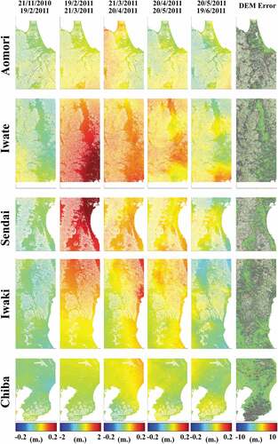
In Table 3, we present the number of pixels identified in the TSPs final subset. Also, we identify the number of TSPs pixels that were rejected as TCPs subset, because their spatial coherence is less than 0.2. These pixels are considered the achieved improvements in the coverage area by using TSPs, which ranges from nearly 25% to 70% depending on the nature of the region under study.

4.3. Accuracy check

We conducted accuracy verification by comparing the estimated InSAR deformation values at pixels that contain GPS stations with the GPS observed LOS deformations (see Figure 10). To ensure the validation of this process, we used some GPS stations that have not been used in the GPS-based supervised spatial phase filtering. Therefore, for some regions, Aomori and Sendai, the number of GPS stations that have corresponding values in the InSAR deformation maps are too limited to reserve some stations for accuracy verification. For this reason, the accuracy verification process is limited to Iwate, Iwaki, and Chiba regions.

Figure 10. Estimated InSAR deformations vs observed GPS deformations, (a) Iwate region, (b) Iwaki region, and (c) Chiba region.

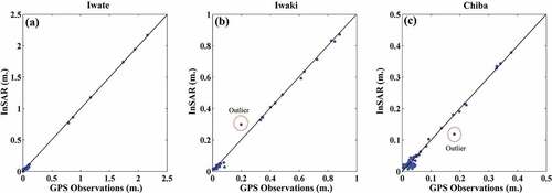
The estimated correlation between the estimated InSAR deformations and GPS observations is nearly 98%: 99%, and the mean Root Mean Square Error (RMSE) in the range of a few millimeters level (Table 4). During the statistical analysis of the accuracy verification results, we set a threshold of $\left(3\mathit{\sigma }\right)$ to remove any outliers that may be leaked to the final results.

Table 4. Statistical analysis of the accuracy check

Region	No. of GPS stations	Mean STD (mm)	Mean RMSE (mm)
Iwate	5	14.0	14.9
Iwaki	10	8.7	8.9
Chiba	15	9.4	10.4
Mean		10.7	11.4

It is expected that the mean RMSE would have a relatively high value (Table 4). This is an anticipated result when comparing GPS observations of a single point (station) with the average return of multilooked pixels. This does not reflect the poor InSAR accuracy but it means that for some pixels the deformations of the targets contained in these pixels are not uniform, which results in some discrepancies when compared with GPS observations.

5. Conclusions

In this paper, we present our approach for monitoring deformations along the East coast of Japan during the coseismic and postseismic activity of the megathrust 2011 Tohoku earthquake using SAR interferometry and GPS observations. The study area is also characterized by its vegetation cover and rough natural terrain. We propose using TSP which we define as the pixels with temporal phase standard deviation equivalent to the expected of a stack of multilooked pixels exhibiting spatial phase coherence of 0.2 in each interferogram of the entire InSAR stack. This definition allows using liberated temporal phase correlation threshold as a selection criterion to identify multilooked pixels with reliable phase returns independent of their varying surrounding pixels that may cause coherence loss.

We present a simulation analysis to relate spatial coherence with temporal phase correlation and found that a temporal phase correlation of 0.53 is equivalent to the expected of a stack of pixels exhibiting spatial coherence of 0.2 with NL of 9. In comparison to pixels with spatial coherence higher than 0.2 for the entire InSAR stack, using TSPs in multi-looked pixels, with a liberal temporal correlation threshold of 0.53, increases the spatial coverage index and the number of identified usable pixels by an average of 36.8% and 50.4%, respectively, for the study area.

We describe in detail the steps of our proposed methodology, which was designed specifically to monitor deformations for the unprecedented event of the 2011 Tohoku earthquake. We start by selecting TSPs’ first subset and use it in cooperation with GPS observations to correct the errors in InSAR stack. Then, we choose a final subset of TSP and use the L1-norm optimization problem to solve for deformations.

We illustrate our approach to incorporate GPS data with InSAR analysis, starting with atmospheric correction, phase unwrapping and supervised spatial phase filtering. We use the L1-norm to solve for deformations which is much robust than the L2-norm against outliers.

Although we use GPS data in several stages, it is not essential for the application of our approach in any study area. The only reason for using GPS data is the dominating nature of the deformation associated with the 2011 Tohoku earthquake which left no stable regions to relate the interferometric deformations.

We apply the proposed methodology to estimate the full coseismic and postseismic deformation signature of the 2011 Tohoku earthquake in the East coast of Japan. We verified the results against GPS observations, which show a mean RMSE of 11.4 mm and a correlation of 98%. These results demonstrate the accuracy and reliability of the proposed approach, taking into consideration the massive magnitude of the 2011 Tohoku Earthquake and the fact that comparing the average results of multilooked pixels against single GPS points should allow some tolerance.

The final results show the differential postseismic deformation pattern that agrees with the other studies, suggesting the occurrence of anomalous crustal strain in Tohoku region as a result of the 2011 Tohoku earthquake.

Disclosure statement

The authors declare that they have no known competing financial interests or personal relationships that could have appeared to influence the work reported in this paper.

Data availability statement

The data that support the findings of this study are openly available in Geospatial Information Authority of Japan (GSI) at [https://www.gsi.go.jp/ENGLISH/] and European Space Agency at [https://earth.esa.int/eogateway/].

Additional information

Funding

This work is supported by Japanese Government (Monbukagakusho, MEXT) Scholarship in 2012.

Notes on contributors

Tamer ElGharbawi

Tamer ElGharbawi is an assistant professor in Department of Civil Engineering, Suez Canal University, Egypt. He received the PhD degree from Kyoto University, Japan. His research interests are hazard management and estimation using remote sensing techniques.

Masayuki Tamura

Masayuki Tamura is a professor emeritus of Kyoto University, Japan. His research interests are signal and image processing.

References

- Bamler, R., and D. Just. 1993. “Phase Statistics and Decorrelation in SAR Interferograms.” Proceedings of IGARSS ‘93 - IEEE International Geoscience and Remote Sensing Symposium, Tokyo, Japan, 980–984. doi:10.1109/IGARSS.1993.322637.
- Blanco-Sánchez, P., J.J. Mallorquí, S. Duque, and D. Monells. 2008. “The Coherent Pixels Technique (CPT): An Advanced DInSAR Technique for Nonlinear Deformation Monitoring.” Pure and Applied Geophysics 165 (6): 1167–1193. doi:10.1007/s00024-008-0352-6.
- Buckley, S.M., P.A. Rosen, S. Hensley, and B.D. Tapley. 2003. “Land Subsidence in Houston, Texas, Measured by Radar Interferometry and Constrained by Extensometers.” Journal of Geophysical Research 108 (B11): 2542. doi:10.1029/2002JB001848.
- Costantini, M., and P.A. Rosen. 1999. “A Generalized Phase Unwrapping Approach for Sparse Data.” IEEE 1999 International Geoscience and Remote Sensing Symposium. IGARSS’99 (Cat. No.99CH36293), Hamburg, Germany, 267–269. doi:10.1109/IGARSS.1999.773467.
- Crosetto, M., B. Crippa, and E. Biescas. 2005. “Early Detection and In-depth Analysis of Deformation Phenomena by Radar Interferometry.” Engineering Geology 79 (1): 81–91. doi:10.1016/j.enggeo.2004.10.016.
- Davis, J.L., T.A. Herring, I.I. Shapiro, A.E.E. Rogers, and G. Elgered. 1985. “Geodesy by Radio Interferometry: Effects of Atmospheric Modeling Errors on Estimates of Baseline Length.” Radio Science 20 (6): 1593–1607. doi:10.1029/RS020i006p01593.
- ElGharbawi, T., and M. Tamura. 2014a. “Measuring Deformations Using SAR Interferometry and GPS Observables with Geodetic Accuracy: Application to Tokyo, Japan.” ISPRS Journal of Photogrammetry and Remote Sensing 88 (1): 156–165. doi:10.1016/j.isprsjprs.2013.12.005.
- ElGharbawi, T., and M. Tamura. 2014b. “Surface Deformation Monitoring Using SAR Interferograms and GPS Observables: Application to Tokyo, Japan.” 2014 IEEE International Geoscience and Remote Sensing Symposium, Quebec City, QC, Canada, 990–993. doi:10.1109/IGARSS.2014.6946593.
- ElGharbawi, T., and M. Tamura. 2015. “Coseismic and Postseismic Deformation Estimation of the 2011 Tohoku Earthquake in Kanto Region, Japan, Using InSAR Time Series Analysis and GPS.” Remote Sensing of Environment 168: 374–387. doi:10.1016/j.rse.2015.07.016.
- ElGharbawi, T., and M. Tamura. 2019. “Increasing Insar Coverage in Vegetated and Rough Terrain Using Temporal Stable Pixels.” 2019 IEEE International Geoscience and Remote Sensing Symposium, Yokohama, Japan, 2115–2118, doi: 10.1109/IGARSS.2019.8898627.
- Ferretti, A., A. Monti-Guarnieri, C. Prati, F. Rocca, and D. Massonet. 2007. “InSAR Principles: Guidelines for SAR Interferometry Processing and Interpretation“. ESATM, 19 . The Netherlands: ESA Publications.
- Ferretti, A., C. Prati, and F. Rocca. 2000. “Nonlinear Subsidence Rate Estimation Using Permanent Scatterers in Differential SAR Interferometry.” IEEE Transactions on Geoscience and Remote Sensing 38 (5): 2202–2212. doi:10.1109/36.868878.
- Ferretti, A., C. Prati, and F. Rocca. 2001. “Permanent Scatterers in SAR Interferometry.” IEEE Transactions on Geoscience and Remote Sensing 39 (1): 8–20. doi:10.1109/36.898661.
- Goldstein, R.M., and C.L. Werner. 1998. “Radar Interferogram Filtering for Geophysical Applications.” Geophysical Research Letters 25 (21): 4035–4038. doi:10.1029/1998GL900033.
- Goldstein, R.M., H. Engelhardt, B. Kamb, and R.M. Frolich. 1993. “Satellite Radar Interferometry for Monitoring Ice Sheet Motion: Application to an Antarctic Ice Stream.” Science 262 (5139): 1525–1530. doi:10.1126/science.262.5139.1525.
- Hagberg, J.O., L.M.H. Ulander, and J. Askne. 1995. “Repeat-pass SAR Interferometry over Forested Terrain.” IEEE Transactions on Geoscience and Remote Sensing 33 (2): 331–340. doi:10.1109/36.377933.
- Hanssen, R.F. 2001. Radar Interferometry: Data Interpretation and Error Analysis. Amsterdam: Kluwer Academic Publishers.
- Hetland, E.A., P. Musé, M. Simons, Y.N. Lin, P.S. Agram, and C.J. DiCaprio. 2012. “Multiscale InSAR Time Series (Mints) Analysis of Surface Deformation.” Journal of Geophysical Research 117 (B2): B02404. doi:10.1029/2011JB008731.
- Hooper, A., P. Segall, and H. Zebker. 2007. “Persistent Scatterer Interferometric Synthetic Aperture Radar for Crustal Deformation Analysis, with Application to Volcán Alcedo, Galápagos.” Journal of Geophysical Research 112 (B7). doi:10.1029/2006JB004763.
- Hopfield, H.S. 1969. “Two-quartic Tropospheric Refractivity Profile for Correcting Satellite Data.” Journal of Geophysical Research 74 (18): 4487–4499. doi:10.1029/JC074i018p04487.
- Huber, P.J. 1987. “The Place of the L1-norm in Robust Estimation.” Computational Statistics & Data Analysis 5 (4): 255–262. doi:10.1016/0167-9473(87)90049-1.
- Imakiire, T., and T. Kobayashi. 2011. “The Crustal Deformation and Fault Model of the 2011 off the Pacific Coast of Tohoku Earthquake.” Bulletin of the Geospatial Information Authority of Japan 59: 21–30.
- Lauknes, T.R., H.A. Zebker, and Y. Larsen. 2011. “InSAR Deformation Time Series Using an L1-Norm Small-Baseline Approach.” IEEE Transactions on Geoscience and Remote Sensing 49 (1): 536–546. doi:10.1109/TGRS.2010.2051951.
- Liu, G., S.M. Buckley, X. Ding, Q. Chen, and X. Luo. 2009. “Estimating Spatiotemporal Ground Deformation With Improved Persistent-Scatterer Radar Interferometry.” IEEE Transactions on Geoscience and Remote Sensing 47 (9): 3209–3219. doi:10.1109/TGRS.2009.2028797.
- López-Quiroz, P., M.-P. Doin, F. Tupin, P. Briole, and J.-M. Nicolas. 2009. “Time Series Analysis of Mexico City Subsidence Constrained by Radar Interferometry.” Journal of Applied Geophysics 69 (1): 1–15. doi:10.1016/j.jappgeo.2009.02.006.
- Massonnet, D., K. Feigl, M. Rossi, and F. Adragna. 1994. “Radar Interferometric Mapping of Deformation in the Year after the Landers Earthquake.” Nature 369 (6477): 227–230. doi:10.1038/369227a0.
- Meyer, F., R. Bamler, N. Jakowski, and T. Fritz. 2006. “The Potential of Low-Frequency SAR Systems for Mapping Ionospheric TEC Distributions.” IEEE Geoscience and Remote Sensing Letters 3 (4): 560–564. doi:10.1109/LGRS.2006.882148.
- Mora, O., J.J. Mallorqui, and A. Broquetas. 2003. “Linear and Nonlinear Terrain Deformation Maps from a Reduced Set of Interferometric SAR Images.” IEEE Transactions on Geoscience and Remote Sensing 41 (10): 2243–2253. doi:10.1109/TGRS.2003.814657.
- Ohzono, M., Y. Yabe, T. Iinuma, Y. Ohta, S. Miura, K. Tachibana, T. Sato, and T. Demachi. 2012. “Strain Anomalies Induced by the 2011 Tohoku Earthquake (Mw 9.0) As Observed by a Dense GPS Network in Northeastern Japan.” Earth, Planets and Space 64 (12): 1231–1238. doi:10.5047/eps.2012.05.015.
- Onn, F., and H.A. Zebker. 2006. “Correction for Interferometric Synthetic Aperture Radar Atmospheric Phase Artifacts Using Time Series of Zenith Wet Delay Observations from a GPS Network.” Journal of Geophysical Research 111 (B9): B09102. doi:10.1029/2005JB004012.
- Paige, C.C., and M.A. Saunders. 1982. “LSQR: An Algorithm for Sparse Linear Equations and Sparse Least Squares.” ACM Transactions on Mathematical Software 8 (1): 43–71. doi:10.1145/355984.355989.
- Rodriguez, E., and J.M. Martin. 1992. “Theory and Design of Interferometric Synthetic Aperture Radars.” IEE Proceedings F Radar and Signal Processing 139 (2): 147–159. doi:10.1049/ip-f-2.1992.0018.
- Saastamoinen, J. 1972. “Contributions to the Theory of Atmospheric Refraction.” Journal of Geodesy 105 (1): 279–298. doi:10.1007/BF02521844.
- Schlossmacher, E.J. 1973. “An Iterative Technique for Absolute Deviations Curve Fitting.” Journal of the American Statistical Association 68 (344): 857–859. doi:10.2307/2284512.
- Sun, T., K. Wang, T. Iinuma, R. Hino, J. He, H. Fujimoto, M. Kido, et al. 2014. “Prevalence of Viscoelastic Relaxation after the 2011 Tohoku-oki Earthquake.” Nature 514 (7520): 84–87. doi:10.1038/nature13778.
- Zhang, L., X. Ding, and Z. Lu. 2011. “Modeling PSInSAR Time Series without Phase Unwrapping.” IEEE Transactions on Geoscience and Remote Sensing 49 (1): 547–556. doi:10.1109/TGRS.2010.2052625.
- Zhang, L., X. Ding, Z. Lu, H.-S. Jung, J. Hu, and G. Feng. 2014. “A Novel Multitemporal InSAR Model for Joint Estimation of Deformation Rates and Orbital Errors.” IEEE Transactions on Geoscience and Remote Sensing 52 (6): 3529–3540. doi:10.1109/TGRS.2013.2273374.
- Zhang, L., Z. Lu, X. Ding, H.-S. Jung, G. Feng, and C.-W. Lee. 2012. “Mapping Ground Surface Deformation Using Temporarily Coherent Point SAR Interferometry: Application to Los Angeles Basin.” Remote Sensing of Environment 117: 429–439. doi:10.1016/j.rse.2011.10.020.