Calibration of GRACE on-board accelerometers for thermosphere density derivation

ABSTRACT

Low Earth Orbit satellite on-board accelerometers play an important role in improving our understanding of thermosphere density; however, the accelerometer-derived densities are subject to accelerometer calibration errors. In this study, two different dynamic calibration schemes, the accelerometer parameter-incorporated orbit fitting and precise orbit determination (POD), are investigated with the Gravity Recovery And Climate Experiment (GRACE) satellite accelerometers for thermosphere density derivation during years 2004–2007 (inclusive). We show that the GRACE accelerometer parametrization can be optimized by fixing scale coefficients and estimating biases every 60 min so that the orbit fitting and POD precision can be improved from 10 cm to 2 cm in the absence of empirical acceleration compensations and as a result the integrity of calibration parameters may be reserved. The orbit-fitting scheme demonstrates similar calibration precision with respect to POD. Their bias estimates in the along-track and cross-track components exhibit an offset within 0.1% and a standard deviation (STD) less than 0.3%. Correspondingly, a bias of 2.20% and a STD of 5.75% exists between their thermosphere density estimates. The orbit-fitting and POD-derived thermosphere densities are validated through the comparison against the results published by other institution. The comparison shows that either of them can achieve a precision level at 6%. To derive thermosphere density from the rapid-increasing amount of on-board accelerometer data sets, it is suggested to take full advantage of the orbit-fitting scheme due to its high efficiency as well as high precision.

KEYWORDS:

• GRACE accelerometer calibration
• thermosphere density
• precise orbit determination
• orbit fit

1. Introduction

Accelerometers onboard the Low Earth Orbit (LEO) satellites, through providing high accuracy measurements of the nonconservative accelerations acting on the satellites, have been extensively investigated and substantially contributed to the derivation of the Earth gravity field (Reigber et al. 2002; Chen et al. 2005) and thermosphere total mass density (Bruinsma, Tamagnan, and Biancale 2004; Sutton, Forbes, and Nerem 2005; Bruinsma et al. 2006; Sutton, Nerem, and Forbes 2007; Doornbos et al. 2012; Jin, Calabia, and Yuan 2018). The precision of the accelerometers carried on the Gravity Recovery And Climate Experiment (GRACE) satellites can reach the level of ${10}^{-9}\mathrm{m}{\mathrm{s}}^{-2}/\sqrt{\mathrm{H}\mathrm{z}}$ for the less-sensitive axis and ${10}^{-10}\mathrm{m}{\mathrm{s}}^{-2}/\sqrt{\mathrm{H}\mathrm{z}}$ for the high-sensitive axes (Frommknecht 2007; Flury, Bettadpur, and Tapley 2008). However, due to variations of the proof mass voltage of the accelerometer as well as the variations of the on-board environments, the acceleration measurements usually require scale and bias calibration before application. For GRACE satellites, the scale errors are typically at 2–8% level while the bias errors can reach at 10⁻⁵ m/s² magnitude and vary with time (Bettadpur 2003; Klinger and Mayer-Gürr 2016). These errors will contaminate the gravity and the thermosphere density signals represented by the accelerometer data. Thus, it is necessary to calibrate the onboard accelerometer measurements before applying them.

Many studies have been carried out on the onboard accelerometer calibration, among which the approaches incorporated accelerometer parameter into satellite dynamics are investigated (Bruinsma, Biancale, and Perosanz 2007; Van Helleputte and Visser 2008; Van Helleputte, Doornbos, and Visser 2009; Bezděk 2010; Visser and Vanden Ijssel 2016; Guo et al. 2018; Vielberg et al. 2018). In such calibration process, the nonconservative accelerations are represented by the accelerometer measurements and their calibration parameters. With the input of accelerometer measurements, the calibration parameters are estimated in the process of gravity field recovery or orbit determination (Reigber et al. 2002; Bruinsma et al. 2003).

LEO-based accelerometer measurements have been widely investigated in gravity field recovery studies and require calibration as well. During such gravity estimation process, the LEO satellite accelerations are obtained from numerical differentiation of kinematic orbits that is fully free from any a priori force models. The accelerations are then divided into two parts, the gravitational part principally parameterized for gravity and the nongravitational part represented by the accelerometer measurements and their calibration parameters (Gerlach et al. 2003). However, gravity inversion is a very time-consuming task and brings about huge computation burden for those who only need calibrated accelerometer data for thermosphere studies.

Another typical implementation of the dynamic calibration method is to estimate calibration parameters within a reduced-dynamic precise orbit determination (POD) process (Van Helleputte and Visser 2008; Van Helleputte, Doornbos, and Visser 2009; Koch, Shabanloui, and Flury 2019). During POD, the nongravitational accelerations usually represented by the empirical models such as drag and solar radiation are replaced by the accelerometer measurements. The principle of this method is that only when the calibration parameters are accurately determined, the dynamic orbits calculated from integrations of the satellite accelerations are accurate. Due to the strong anticorrelations between scale and bias factors, Van Helleputte, Doornbos, and Visser (2009) applied very strong constraints on the bias parameters in radial and cross-track directions when calibrating the GRACE accelerometers. When accelerometer data were used and no empirical accelerations were estimated, the root mean square (RMS) value of the GRACE satellite orbit differences was just around 10 cm compared to the Jet Propulsion Laboratory (JPL) precision scientific orbit (PSO). To further improve the orbit precision, empirical acceleration models in along-track, cross-track, and radial directions were introduced to absorb any un-/mis-modeled accelerations in their studies. By such dynamic modeling, the GRACE orbit precision could be improved to an RMS value of 3.5 cm. It is also found that the calibration factors in along-track component can be well determined due to its strong signal strength by atmospheric drag, but the radial component is barely meaningful. However, though the orbit precision reaches a higher level by estimating empirical accelerations, the estimated bias or scale parameters are no longer complete as the part of the calibration parameters can be absorbed in the empirical accelerations (personal communication, Bruinsma Sean). In addition, this method also requires the processing of raw GPS data sets, which increases complexity.

Bezděk (2010) proposed another method for on-board accelerometer calibration that compares accelerometer data with the nongravitational accelerations obtained by subtracting the gravitational accelerations from total accelerations using background models. The satellite total accelerations were calculated from numerical differentiation of kinematic orbits. However, due to the errors in kinematic orbits as well as the error amplification and correlation through numerical differentiation, this method strongly depends on the following factors: (1) accurate calculation of satellite accelerations from kinematic orbits; (2) an autoregressive process to account for correlated errors; and (3) the accuracy of background gravitational models. Bezděk (2010) applied a second-derivative filter for orbit derivatives and the generalized least squares for estimation as it allows for joint estimation of calibration parameters and correlated errors, hence to produce realistic GRACE calibration parameters in agreement with Bettadpur (2003). Vielberg et al. (2018) reinvestigated this calibration method with the GRACE on-board data and refined it by using derived nongravitational accelerations as observations for direct estimation of calibration parameters as well as applying an autoregressive process to account for the correlation errors. In a similar approach, Wöske et al. (2019) calibrated the GRACE accelerometer straightforward by nongravitational force modeling using start-of-the-art models. In such procedure, nongravitational forces had to be handled very carefully, including the atmospheric drag forces and winds, as well as radiation forces due to solar radiation pressure, albedo, Earth infrared and satellite thermal radiation; and the high-precision satellite-surface model such as finite element model should be utilized for forces modeling. However, due to limited satellite drag model accuracy, this approach cannot produce precise along-track calibrations, e.g. for GRACE satellites the fitting residuals were around 10 nm/s² for total accelerations around ±70 nm/s² at low solar activity (Wöske et al. 2019); thus, it is not a suitable choice for thermosphere density retrieval that mainly depends on along-track accelerometer observations.

To date, a number of LEO missions are equipped with accelerometers on board, such as Gravity field and steady-state Ocean Circulation Explorer (GOCE), Swarm, GRACE follow-on, etc. The accuracy and efficiency of accelerometer calibration are both critical for accelerometer-based thermosphere density retrieval studies. An error of 10 nm/s² in the accelerometer measurements in the along-track component can lead to density retrieval errors at 2–3% level at the altitude of CHAMP (CHAllenging Minisatellite Payload) satellite (Doornbos 2012). Based on this, we explored another dynamic calibration scheme, which incorporates the accelerometer data into orbit fitting. In this method, the modeled gravitational accelerations and the accelerometer data are used in orbit integration to produce orbit that best fits the reference orbit, while the calibration parameters are estimated during the fitting process together with the satellite initial state vectors. In many orbit determination software such as PANDA (Liu and Ge 2003), orbit fitting is often used for preparing approximate initial state vectors and dynamic parameters. Thus, calibration through orbit fitting is simple to implement. In addition, the orbit-fitting method can achieve much higher efficiency than the methods proposed by Van Helleputte, Doornbos, and Visser (2009) since there is no need to process the on-board GPS data.

The GRACE L1B products from 2004 to 2007 (inclusive) are used for investigating the dynamic calibration methods. Mainly the POD and orbit-fitting calibration schemes are explored and evaluated. Data processing strategies are discussed and analyzed comprehensively, especially on the parameterization of calibration parameters. The two sets of calibration results are compared and their precision is assessed. The following sections are organized as below: the GRACE data and calibration methods are introduced in Section 2; the data processing strategy, especially the dynamic models, is discussed in Section 3; parameterization of the GRACE accelerometer measurements is analyzed in Section 4; in Section 5, the calibration results from POD and orbit fitting are presented and compared; in Section 6, the results of thermosphere density derivation using the two calibration schemes are presented and their precisions are validated; then the conclusions are given in Section 7.

2. Materials and methods

In this section, the data sources involved in the calibration procedure are introduced, and then the two dynamic calibration methods, orbit fitting and POD, are presented.

2.1. GRACE satellite data

The GRACE Level-1B (L1B) products from 2004 to 2007 are retrieved from the Information System and Data Center (ISDC) for this study (Case, Kruizinga, and Wu 2010). The L1B level products include measurements from different onboard sensors. In this study, the GPS data, accelerometer data, and star camera data are employed. The GRACE accelerometer data from L1B products is given in the satellite body-fixed frame (SBF; its definition is depicted in Figure 1) (Case, Kruizinga, and Wu 2010; Dahle et al. 2013). The L1B star camera measurements, which describe the satellite attitude using quaternions, are used to convert coordinates between SBF and the celestial reference frame (CRF).

Figure 1. GRACE satellite SBF definition (Doornbos 2012).

The GRACE GPS measurements are utilized during the POD calibration scheme. The GPS satellite orbit and clock products are also required in a GPS-based POD process. The 30 s GPS clock products that allow to reduce interpolation errors and the orbit products from JPL second IGS reprocessing campaign (repro2) are adopted (Desai et al. 2014). Since the JPL repro2 products are generated with the same configurations and models, they are more consistent than the legacy IGS products. However, it may increase orbit differences between the POD results and the GRACE PSO as they are generated using different GPS products.

The JPL GRACE PSO product (namely the GNV products) is obtained from typical reduced-dynamic POD procedure, which is represented by a set of background models and dynamic parameters. Fitting to the JPL PSO equals to fitting the accelerometer data backward to the dynamic models. In contrast, it is more appropriate to use kinematic orbits for orbit fitting as they are free from any a priori models. In our study, the GRACE kinematic orbits produced by Graz University of Technology are adopted for orbit fitting (Zehentner and Mayer-Gürr 2015). These orbits are calculated using raw undifferenced GPS observables with a kinematic orbit determination technique and are free from any dynamic models. They are considered to have an accuracy of 2–3 cm, which is sufficient for the calibration.

The orbit precision is regarded as a metric when evaluating the calibration performance. The GRACE orbit generated with calibrated acceleration observables is compared with the JPL PSO and validated with the satellite laser ranging (SLR) observations. The statistics of orbit differences and SLR residuals are then used for orbit precision assessment. The smaller the orbit discrepancy and SLR residuals are, the more accurate the calibration parameters are.

2.2. Accelerometer calibration by orbit fitting

The original accelerometer measurements refer to the accelerometer frame, whereas L1B accelerometer products are in SBF. For orbit calculations in the orbit-fitting procedure, all satellite accelerations are represented in CRF. We convert the L1B accelerometer data from SBF to CRF using attitude transformation matrix calculated by the L1B attitude products

(1) ${\tilde{a}}_{CRF}=M\left(b+Ka\right)$(1)

where M is the attitude matrix. For calculating M with GRACE attitude data, please refer to Case, Kruizinga, and Wu (2010). b is the 3 × 1 bias vector consisting the accelerometer biases in SBF X, Y, Z components, while K is the scale factor matrix with a dimension of 3 × 3. a is the acceleration measurements in SBF, while ${\tilde{a}}_{CRF}$ is the calibrated accelerations in CRF. Both a and ${\tilde{a}}_{CRF}$ are three-dimensional vectors representing the acceleration components in X, Y, Z directions. To estimate the bias and scale factors, the partial derivatives of acceleration with respect to b and K need to be calculated when generating a priori dynamic orbit by numerical orbit integration, and they can be deduced from Equation (1)(1) ${\tilde{a}}_{CRF}=M\left(b+Ka\right)$(1) as below:

(2) $\frac{\mathrm{\partial }{\tilde{a}}_{CRF}}{\mathrm{\partial }b}=M$(2)

(3) $\frac{\mathrm{\partial }{\tilde{a}}_{CRF}}{\mathrm{\partial }K}=Ma$(3)

In the orbit-fitting scheme, the positions from kinematic orbit $r_t^{\mathrm{o}\mathrm{b}\mathrm{s}}$ at epoch $t$ are treated as pseudo-observations for the satellite positions $r_t$. Thus, the observation equation can be formed as

(4) ${\mathit{r}}_t^{\mathrm{o}\mathrm{b}\mathrm{s}}={\left.{\mathit{r}}_t\right|}_{{\mathit{x}}_0}+{\mathit{v}}_t$(4)

In Equation (4)(4) ${\mathit{r}}_t^{\mathrm{o}\mathrm{b}\mathrm{s}}={\left.{\mathit{r}}_t\right|}_{{\mathit{x}}_0}+{\mathit{v}}_t$(4) , $x_0$ are the parameters needed to be estimated, including the initial satellite position and velocity at beginning epoch $t_0$ as well as the accelerometer calibration parameters b and K. ${\left.{\mathit{r}}_t\right|}_{{\mathit{x}}_0}$ are the satellite positions taken from a priori dynamic orbit calculated with $x_0.v_t$ is the observation error. Expanding $r_t$ in Equation (4)(4) ${\mathit{r}}_t^{\mathrm{o}\mathrm{b}\mathrm{s}}={\left.{\mathit{r}}_t\right|}_{{\mathit{x}}_0}+{\mathit{v}}_t$(4) using the Taylor’s theorem at $t_0$, and then expressing them in a matrix form for subsequent adjustment, we have

$v_t=A_t\mathrm{\Delta }{x}_0-l_t$

(5) ${\mathit{l}}_t={\mathit{r}}_t^{\mathrm{o}\mathrm{b}\mathrm{s}}-{\left.{\mathit{r}}_t\right|}_{{\mathit{x}}_0}$(5)

$A_t=\frac{\mathrm{\partial }{r}_t}{\mathrm{\partial }{x}_{\mathrm{t}}}\cdot \frac{\mathrm{\partial }{x}_t}{\mathrm{\partial }{x}_0}$

where $\mathrm{\Delta }{x}_0$ is the correction vector for $x_0$, $A_t$ is the design matrix, equaling to the product of the partial derivatives of satellite positions over satellite state at epoch t ($\frac{\mathrm{\partial }{r}_t}{\mathrm{\partial }{x}_{\mathrm{t}}}$) and the satellite state transition matrix $\frac{\mathrm{\partial }{x}_t}{\mathrm{\partial }{x}_0}$, which can be calculated simultaneously during numerical orbit integration, and $l_t$ is the observed minus computed (OMC) residual vector. For each epoch, the observation equation can be established according to Equation (5)(5) ${\mathit{l}}_t={\mathit{r}}_t^{\mathrm{o}\mathrm{b}\mathrm{s}}-{\left.{\mathit{r}}_t\right|}_{{\mathit{x}}_0}$(5) . Normal equations can be formed by stacking all the observation equations epoch by epoch in a selected orbit arc. Thus, $\mathrm{\Delta }{x}_0$ can be estimated using the least-square adjustment method by

(6) $\mathrm{\Delta }{x}_0={\left(A^{\mathrm{T}}A\right)}^{-1}{A}^{\mathrm{T}}L$(6)

where A and L are the stacked design matrix and residual vectors, respectively. With the obtained corrections $\mathrm{\Delta }{x}_0$, the satellite initial state and accelerometer calibration parameters $x_0$ can then be updated. Since the observation equation is not a linear system, 3–4 times of iterations of above procedure is often required to achieve convergence. The final estimates $x_0$ represent the dynamic orbit that best fits the kinematic orbit.

2.3. Accelerometer calibration by POD

Accelerometer calibration in a GPS-based POD procedure differs with the orbit-fitting scheme in the respect of observation equation modeling. In the POD scheme, the GPS observations, including the pseudorange and carrier phase, are modeled with respect to the dynamic orbit. The estimated parameters include not only the initial satellite state and accelerometer calibration parameters, but also the receiver clock errors and ambiguities. In our study, the ionosphere-free pseudorange and carrier phase are utilized for observation equation modeling, which allows for elimination of the first-order ionosphere refraction delays. For a detailed description on GPS-based POD procedure, the readers are referred to Montenbruck and Gill (2000) and Jäggi et al. (2007).

3. Data processing strategy

The performances of orbit-fitting and POD calibration schemes both significantly depend on the satellite dynamic configurations, which means that the fitting or POD arc length and dynamic models can all affect the final calibration precision. In the GFZ GRACE Level 2 data processing standard documents, the detailed strategy for recovering Earth Gravity using GRACE data is described. In the early versions of these standards (0001/0002), the arc length was set 36 h while in more recent versions (0003/0004/0005) was 24 h (Dahle et al. 2013). In this study, the 24 h arc length is selected. The gravitational errors can be minimized by adopting background models as accurate as possible, such as utilizing the EIGEN-6C model for both static and time-varying gravity field (Foerste et al. 2011), FES2004 model for ocean tide (Lyard et al. 2006).

For the GRACE satellites, the accelerometer scales and biases cannot be estimated simultaneously without applying constraints due to their strong correlation (Bruinsma, Biancale, and Perosanz 2007; Van Helleputte, Doornbos, and Visser 2009). To solve this problem, Van Helleputte and Visser (2008, 2009) applied strong constraints on the a priori bias values in the cross-track and radial direction. Bruinsma, Biancale, and Perosanz (2007) found no significant variability of bias factors when strong constraints applied on scale factors, which supports the idea of fixing scales to constant values and estimating only biases. Such accelerometer parameterization is also consistent with the strategy proposed in Dahle et al. (2013).

The accelerometer biases are often estimated typically one set per single day (e.g. Van Helleputte and Visser 2008; Van Helleputte, Doornbos, and Visser 2009; Vielberg et al. 2018). But according to Van Helleputte and Visser (2008, 2009), the orbit precision estimated in such strategy can only reach at 10 cm level when no empirical accelerations are applied, which is significantly degraded compared to the GRACE POD results reported in other studies (Kang et al. 2006; Jäggi et al. 2007). Even though the precision is much improved after introducing the empirical accelerations, the bias estimations are subject to nontrivial deviation as the empirical accelerations and the biases are correlated. In the GFZ processing standard release 0005, it is suggested the scale factors are kept as constants while the biases are estimated every 60 min (Dahle et al. 2013). In addition, there could also be other couplings in the biases, e.g. a dependence on temperature. In our calibration strategy, the temperature-induced biases variations can be absorbed by the piecewise-constant biases and then represented in long-term trend. It should also be noted that the GRACE satellite thermal control during 2004–2007 was in a good condition and thus the thermal coupling effects were small. Thus, these technical couplings can be ignored at this point.

For the orbit-fitting scheme, the kinematic positions are treated as pseudo-observations. However, when performing POD calibration scheme, certain errors in GPS observations should be taken into consideration. Hence, the GPS observation model configurations can impact the POD calibration precision. To minimize the orbit discrepancies with respect to the JPL PSO, similar models are adopted to form the on-board GPS observation equation.

Table 1 lists the detailed dynamic and observation models for both orbit-fitting and POD calibration schemes. The EIGEN-6C model is adopted to calculate the Earth’s gravity, including both static and periodic terms. The solid Earth tide, pole tide are calculated using models recommended by IERS 2003 (McCarthy and Petit 2004). Ocean tide is computed using the FES 2004 model, while the atmosphere tide using GRACE AOD products with degree and order of 40. Particularly, the accelerometer data is first calibrated using the approximations provided in Bettadpur 2003, and then used in orbit integration. Different bias intervals for accelerometer are explored, and the results are given in Section 4. We use the ionospheric-free combination (PC: code combination, LC: phase combination) to eliminate the first-order ionosphere delay while the second and higher orders are neglected. The JPL repro2 precision GPS ephemeris and 30 s clock products are adopted for GPS satellite positions and clock errors. GPS satellite antenna phase center offset (PCO) and phase center variations (PCVs) are corrected using IGS antenna models (Schmid et al. 2005), while the receiver antenna PCO is corrected using the values provided by ISDC VOGPSN products (Case, Kruizinga, and Wu 2010).

Table 1. Processing strategy in aspects of dynamic models and observation models

Dynamic models
Gravity Model	EIGEN_6C, 130 × 130 for static field and periodic terms
Solid Earth tide and pole tide	IERS2003
Ocean tide	FES2004 40 × 40
N-body perturbation	JPL DE405; planets include sun, moon, Mercury, Venus, Mars, Jupiter, Saturn, Uranus, Neptune and Pluto
Atmosphere gravity	GRACE Atmosphere Ocean De-aliasing (AOD) (Release-0005) products 40 × 40
Relativity	IERS 2003
Nongravitational accelerations such as drag and radiations	Represented by accelerometer data
Observation model
Observation	PC, LC
Arc length and interval	24 h, 30 s
GPS ephemeris and clock	JPL repro2 precision orbit and clock products; fixed
Ionosphere delay	First-order delay eliminated by ionosphere-free combination, higher orders are neglected
GPS satellite antenna PCO, PCV	IGS ATX
GRACE satellite receiver antenna PCO/PCV	PCO corrected using VOGPSN product, PCV not considered
Relativistic effect	Bending and Sagnac effect
Estimating Parameters
GRACE initial state	Estimated with a-priori deviation of 1000 m and 1 m/s for positions and velocities, respectively
Accelerometer bias	Estimated as piecewise-constant at specific time interval with a priori deviation of 1 μm/s^2
Phase ambiguity	Estimated as constants per each continuous arc with a priori deviation of 10 m
Receiver clock error	Estimated as random-walk parameters per epoch with a priori deviation and a priori process noise of 9000 m and $900\mathrm{m}/\sqrt{\mathrm{s}}$, respectively

4. Parameterization for accelerometer measurement

To evaluate the parameterization for accelerometer measurements, we processed the GRACE-A satellite data from day of year (DOY) 100 to 150 in 2006 (the time system is GPS Time) using the orbit-fitting calibration scheme with different estimation interval for bias factors. Dynamic models are adopted as listed in Table 1 with the estimation interval for the bias factor set as 45, 60 , 90, 180, and 360 min (respectively indicated as acc_45, acc_60, acc_90, acc_180, and acc_360 hereafter), in which 90 min is just about one orbit period of the GRACE satellites, 45, 180, and 360 min are the half, double, and quadruple of GRACE orbit period, respectively, while the 60 min interval is tested here as it is recommended in Dahle et al. 2013.

After orbit fitting, the reduced-dynamic orbit generated from the fitted state vectors and calibration parameters is compared to the JPL PSO and validated by the SLR technique. The parameterization that gives highest precision statistics results will be considered as the best scheme against others. The 24 h estimation interval is not tried here as Van Helleputte and Visser (2008, 2009) have already shown that the orbit precision can only reach 8.8 cm with respect to the JPL PSO.

4.1. Orbit precision comparison for different bias intervals

Figure 2 illustrates the RMS values of the orbit difference comparing to JPL PSO with different estimation intervals for each arc. The precision in the radial and along-track direction of all the five cases is very similar and their RMS series fluctuate steadily and smoothly except the results on DOY 112/2006 for cases acc_45 and acc_90. Generally, the radial and along-track precision is around 1.0 and 2.0 cm, respectively. However, the precision of cross-track component reaches around 1.5 cm for 45 min and 60 min interval, but degrades significantly to about 2.0–5.0 cm when the estimation interval is increased to 90,, 180, and 360 min. A very large orbit difference RMS for the arc in DOY 113 is noticed in all three components for case acc_45 and in cross-track component for case acc_90. This is possibly related to that there are no available kinematic orbit positions during 07:52:50–09:00:00 on 23 April 2006 (DOY 113/2006). In a kinematic POD process, orbit gaps occur quite frequently that is largely due to poor observation quality or data outage, and a variety of factors could induce such results such as strong ionosphere activity, signal loss, receiver reboot, etc. (Montenbruck et al. 2018).

Figure 2. GRACE-A satellite orbit differences with respect to the JPL PSO. Different colors demonstrate different accelerometer bias parameterization.

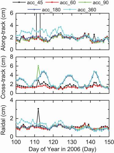
Table 2 shows the mean RMS value of the daily orbit differences for each component. Orbit precision with respect to JPL PSO is roughly all better than 5.0 cm (3D RMS) in all cases if the results on arc DOY 113 are excluded, while using the case of estimation interval 60 min achieves the best orbit precision against the others, which can reach 1.8, 1.4, and 1.0 cm in the along-track, cross-track, and radial directions, respectively. The precision in cross-track direction varies to somewhat larger extent among different cases compared to that in the along-track and radial directions, which might suggest it is more sensitive to the bias parameterization.

Table 2. GRACE-A satellite orbit precision with respect to the JPL PSO and SLR OMC statistics with different accelerometer bias parameterization

Bias parameterization	Orbit comparison to JPL PSO (cm)				SLR OMC (cm)
	Along-track	Cross-track	Radial	3D	Mean	STD
acc_45	4.96 (1.82)	1.62 (1.59)	1.12 (1.08)	5.34 (2.65)	−0.26	2.15
acc_60	1.78	1.35	1.00	2.45	−0.37	1.78
acc_90	1.74	2.66	1.02	3.34	−0.35	2.11
acc_180	1.91	2.60	0.99	3.37	−0.39	2.06
acc_360	2.48	2.65	1.21	3.82	−0.41	2.20

The values in the parentheses indicate the RMS statistics with DOY 112 removed.

The SLR fit is also used here for orbit precision validation. Table 2 shows the mean and STD of SLR residuals for the five cases. There is a bias about 0.2–0.5 cm in all the orbit solutions, and the STDs are all below 2.5 cm. The best precision (1.78 cm) is achieved by acc_60, which is consistent with the orbit comparison results.

The orbit precision in these five cases is very comparable to the result by Van Helleputte, Doornbos, and Visser (2009) that the empirical accelerations are estimated every 600 s in all three directions, but much better than that without estimating empirical accelerations. The 60 min interval gives best performance, which is exactly in agreement with the GFZ processing strategy.

4.2. Comparison of estimated bias parameters

Figure 3 depicts the estimated bias series in X, Y, and Z directions (in SBF, denoted as Bx, By, and Bz hereafter) of the five cases. Since the actual attitudes of GRACE satellites are very close to their nominal ones, Bx, By, and Bz generally indicate biases in the along-track, cross-track and radial components, respectively. Generally, Bx, By, and Bz series are in the same magnitude among different cases. An outlier estimate in cross-track direction for cases 45 and 90 min is observed, which should be attributed to the missing positions from the kinematic ephemeris and is consistent with the orbit RMS statistics in Figure 1. During this period, the Bx, By, and Bz biases from different cases all fluctuate around −1.170 × 10⁻⁶, 2.886 × 10⁻⁵, −5.440 × 10⁻⁷ m/s², respectively, and show very consistent variation trends.

Figure 3. Estimated Bx, By, Bz parameters during DOY 100–150 in 2006 with different parameterizations.

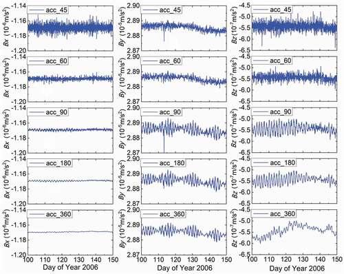
The mean and STD values of the estimated bias parameters are listed in Table 3. The differences of their bias mean values among different cases are quite small, mainly at the magnitude of 10⁻⁹ m/s². The Bx series generally exhibits the smallest amplitude variation among the three components. In addition, its variations reduce significantly when the estimation interval is extended, which is revealed by the STD statistics as well. In the cases of acc_90, acc_180, and acc_360, the Bx estimates are almost constant during the testing period, and their STDs are 1.022 × 10⁻⁹, 6.510 × 10⁻¹⁰, and 4.910 × 10⁻¹⁰ m/s², respectively, while in cases acc_45 and acc_60 the Bx STDs are obviously larger, reaching 4.520 × 10⁻⁹ and 2.078 × 10⁻⁹ m/s², respectively. On the contrary, the By and Bz series from different cases show obviously larger variations. Their STDs are generally at the level of (1–2) × 10⁻⁸ m/s² and grow larger when estimation interval exceeds 60 min. This might be related to several reasons. On one hand, sensitivity of the accelerometer is weakest in the SBF-Y direction; on the other hand, dynamic modeling of GRACE-A satellite is incomplete in our study. The un-/mis-modeled gravitational forces including ignored high-order Earth gravity field (over order and degree of 130) and ocean tidal perturbations (over order and degree of 40) mainly act on the SBF-Z direction. This would result in more variable Bz estimates.

Table 3. The mean and STD values of estimated Bx, By, Bz parameters during DOY 100–150 in 2006

Bias parameterization	Bx (m/s^2)		By (m/s^2)		Bz (m/s^2)
	Mean	STD	Mean	STD	Mean	STD
acc_45	−1.1700 × 10^−6	4.5200 × 10^−9	2.8855 × 10^−5	1.8979 × 10^−8	−5.4400 × 10^−7	1.6800 × 10^−8
acc_60	−1.1691 × 10^−6	2.0788 × 10^−9	2.8855 × 10^−5	1.8966 × 10^−8	−5.4393 × 10^−7	1.4676 × 10^−8
acc_90	−1.1691 × 10^−6	1.0217 × 10^−9	2.8855 × 10^−5	2.7284 × 10^−8	−5.4357 × 10^−7	1.8280 × 10^−8
acc_180	−1.1691 × 10^−6	6.5104 × 10^−10	2.8854 × 10^−5	2.5583 × 10^−8	−5.4382 × 10^−7	1.7553 × 10^−8
acc_360	−1.1691 × 10^−6	4.9096 × 10^−10	2.8853 × 10^−5	2.3874 × 10^−8	−5.4359 × 10^−7	2.2016 × 10^−8

According to Figure 3, in the cases of acc_45 and acc_60, the estimated Bx, By and Bz series mostly give signatures of high-frequency noise pattern. However, they tend to reveal periodical variations in very similar frequencies when estimating in larger intervals, as seen in the cases of acc_90, acc_180, and acc_360. The reason for these periodical signals is still under investigation.

When using accelerometer data for thermosphere derivation, the precision of calibration parameters in the along-track direction is much more important than that in other directions as the satellite drag acceleration mainly acts in this direction. The estimates for Bx from the above test cases all give very similar results except the case acc_45, which tends to overestimate the Bx parameters, likely due to over-parameterization.

5. Comparison of different dynamic calibration schemes

In this section, the GRACE data from 2004 and 2007 were processed and calibrated using the POD and orbit-fitting schemes, respectively. Their calibration results were then compared. According to the test results in the above section, the acc_60 case was selected as dynamic configuration for the GRACE accelerometer parameterization.

5.1. Orbit precision comparison

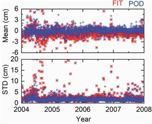
Similar to the above section, the precision of dynamic calibration schemes was firstly evaluated by the orbit precisions. For illustration, the GRACE-A satellite orbits from POD and orbit-fitting schemes were compared to the JPL PSO for each arc, and the RMS values of their orbit differences in along-track, cross-track, and radial components were calculated and are displayed in Figure 4. Generally, the orbit precisions of the two schemes can both reach cm level. Compared to JPL PSOs, the POD results give better agreement in the along-track component than the orbit-fitting method, while they agree in the cross-track direction. The radial component precision of orbit-fitting scheme demonstrates an obvious advantage over the POD scheme. The overall mean RMS values of orbit precisions with respect to JPL PSOs are listed in Table 4. The orbit precision from orbit fitting is 2.21, 1.55, and 1.27 cm in the along-track, cross-track, and radial component, respectively, while that from POD is 1.36, 1.49, and 1.65 cm in the three components. Their 3D position precisions are 2.98 and 2.61 cm, respectively. In general, the POD precision is slightly better than orbit fitting. This should be due to that the state transition constraints during a kinematic orbit determination process are much looser than those during a dynamic orbit determination since the satellite positions must be estimated for every epoch, which can then result in worse orbit precision. As confirmation, we compared the Graz kinematic orbits and the JPL PSOs, which indicates that their differences are 2.31, 2.31, and 2.59 cm in the along-track, cross-track, radial components. This is even worse than the orbit precision of the orbit-fitting scheme. The radial precision from orbit-fitting scheme is better than POD, which might be attributed to that the kinematic positions involved in orbit fitting are vectors along the radial direction, thus making the constraints on this component stronger than others. In addition, the orbit differences show larger discrepancy during the first half year in 2004, which is in agreement with the results given in Zehentner and Mayer-Gürr (2015).

Figure 4. GRACE-A satellite orbit precision for POD and orbit-fitting schemes in along-track, cross-track, and radial components with respect to JPL PSOs.

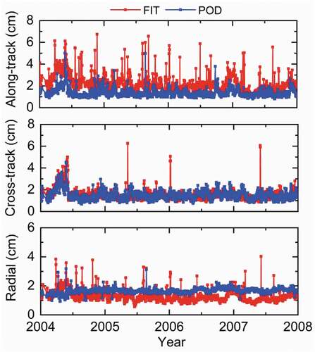
Table 4. GRACE-A satellite orbit precision statistics during 2004–2007

Calibration scheme	Orbit comparison to JPL PSOs (cm)				SLR OMC (cm)
	Along-track	Cross-track	Radial	3D	Mean	STD	RMS
Orbit fitting	2.21	1.55	1.27	2.98	−0.53	2.52	2.58
POD	1.36	1.49	1.65	2.61	0.11	1.92	1.92

The SLR observations are also taken in for orbit precision evaluation of the two schemes. The SLR OMC mean and STD of GRACE-A satellite for each arc are shown in Figure 5, while their mean values are listed in Table 4. For both schemes, the SLR OMC mean values fluctuate mostly in the ranges from −5 to 5 cm and their STDs are mainly below 5 cm. The SLR OMC mean and STD values of orbit-fitting scheme are −0.53 cm and 2.52 cm, which is larger than those of the POD scheme. This is consistent with the orbit comparison results.

Figure 5. SLR OMC mean and STD values of GRACE-A satellite during 2004 and 2007.

5.2. Calibration parameters comparison

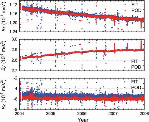
The bias parameters of GRACE-A satellite obtained using the orbit-fitting and POD methods are illustrated in Figure 6. Both schemes reveal noticeable gradual trending changes for the bias parameters especially in the SBF-X and SBF-Y directions, which fluctuate from −1.12 × 10⁻⁶ m/s² to −1.20 × 10⁻⁶ m/s² and from 2.8 × 10⁻⁵ m/s² to 2.9 × 10⁻⁵ m/s², respectively, while the bias parameters in SBF-Z direction vary around −5 × 10⁻⁷ nm/s². The Bx and By parameter time series gives significant signatures of bias drifts, which is consistent with the previous studies (Bruinsma, Biancale, and Perosanz 2007; Van Helleputte, Doornbos, and Visser 2009; Klinger and Mayer-Gürr 2016). For both schemes, the bias drift in the SBF-X component is about 14 nm/s² per year while in the SBF-Y component 200 nm/s² per year. Such drifts could have resulted from mixed reasons. Parts of the drifts can be results of real satellite hardware changes, such as the spacecraft thermal variations in the long-term scale, which has been already reported (Doornbos 2012; Klinger and Mayer-Gürr 2016). Jumps of the bias parameters can be observed for both schemes in some arcs, which should be due to the effects of specific events, such as maneuvers, instrument reboots or switching from main to redundant board and vice versa. Comparing the calibration biases from the two schemes, excellent agreement can be observed in the SBF-X and SBF-Y components. However, there exists a systematic difference in the SBF-Z component between the two schemes. Since we applied the same dynamic models in the orbit-fitting and POD schemes, such systematic Bz differences might be due to the inconsistent handling of the GRACE-A satellite GPS data between our study and the Graz kinematic orbits.

Figure 6. GRACE-A satellite bias parameter series during 2004–2007.

The differences of the bias parameters between the orbit-fitting and POD schemes are illustrated in Figure 7. In comparison, the differences of the Bx parameters are the smallest, which mainly fluctuate within several nm/s². However, the differences in the SBF-Y and SBF-Z components are at much larger magnitude about several tens of nm/s² while an additional offset can be found in the Bz differences. The mean and STD values of the differences are presented in Table 5. For Bx, the mean and STD values of the differences are only 0.52 ± 2.97 nm/s², while they are −1.48 ± 31.82 nm/s² and 42.71 ± 22.63 nm/s² for By and Bz differences, respectively. The small differences in Bx estimates indicate that both schemes can derive thermosphere densities at very similar precision. Treating the bias parameters from orbit-fitting scheme as references, the relative differences between the two schemes are also calculated. For Bx, the relative differences are very small, at −0.04% ± 0.26%, while the Bz parameter differences are as large as −7.25% ± 3.85%.

Figure 7. Bias parameter difference series between the orbit-fitting and POD schemes for GRACE-A satellite.

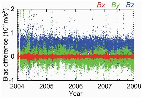
Table 5. GRACE-A satellite bias parameter differences between the orbit-fitting and POD schemes

Components	Mean (nm/s^2)	STD (nm/s^2)	Relative mean (%)	Relative STD (%)
ΔBx	0.52	2.97	−0.04	0.26
ΔBy	−1.48	31.82	0.00	0.11
ΔBz	42.71	22.63	−7.25	3.85

In many previous studies, the GRACE satellite accelerometer calibration parameters are usually estimated on a daily basis (e.g. Van Helleputte and Visser 2008; Van Helleputte, Doornbos, and Visser 2009; Vielberg et al. 2018). To facilitate comparison, we averaged the 60 min Bx, By, and Bz parameters from the orbit-fitting scheme into daily values. The results also demonstrate that for Bx the daily STD is under 4 nm/s² and is mainly less than 0.3% over its daily mean value; for By and Bz, their STDs both vary at a higher level and are typically under 20 nm/s². These daily STD values can represent the bias estimation precision and are also consistent with the results in Vielberg et al. (2018).

6. Comparison of the calibration schemes on thermosphere density derivation

Thermosphere densities are important parameters in modeling the space environment. Deriving thermosphere densities through LEO-on-board accelerometers are attracting greatly increased attention in recent decades due to its good accuracy as well as huge data number. In this section, we investigated thermosphere density derivation using the GRACE accelerometer data by applying the obtained Bx parameters from the two calibration schemes described above. The derived two sets of densities were firstly compared to each other and then compared to the estimates by different approaches, including empirical models as well as densities calculated by other researchers.

To retrieve densities from accelerometer data, mainly the accelerometer measurements of the SBF-X components are explored. Detailed procedures on the density derivation can be found in Bruinsma, Tamagnan, and Biancale 2004; Sutton, Nerem, and Forbes 2007; Doornbos 2012; Vielberg et al. 2018. Firstly, the satellite aerodynamic accelerations are isolated by subtracting the solar radiation pressure (SRP) and Earth radiation pressure from the calibrated accelerometer data. Thus, we have

(7) $a_{X,\mathrm{o}\mathrm{b}\mathrm{s}}=a_{X,\mathrm{c}\mathrm{a}\mathrm{l}}-a_{\mathrm{s}\mathrm{r}\mathrm{p}}-a_{\mathrm{a}\mathrm{l}\mathrm{b}}-a_{\mathrm{I}\mathrm{R}}$(7)

In Equation (7)(7) $a_{X,\mathrm{o}\mathrm{b}\mathrm{s}}=a_{X,\mathrm{c}\mathrm{a}\mathrm{l}}-a_{\mathrm{s}\mathrm{r}\mathrm{p}}-a_{\mathrm{a}\mathrm{l}\mathrm{b}}-a_{\mathrm{I}\mathrm{R}}$(7) , $a_{X,\mathrm{c}\mathrm{a}\mathrm{l}}$ and $a_{X,\mathrm{o}\mathrm{b}\mathrm{s}}$ are the calibration accelerometer data in SBF-X and observed drag acceleration, respectively; the SRP accelerations $a_{\mathrm{s}\mathrm{r}\mathrm{p}}$ is calculated using the GRACE macro model (Bettadpur 2012); the Earth radiation accelerations including albedo $a_{\mathrm{a}\mathrm{l}\mathrm{b}}$ and infrared radiation $a_{IR}$ are calculated using grid model (Bhanderi and Bak 2005). In practice, $a_{\mathrm{a}\mathrm{l}\mathrm{b}}$ and $a_{\mathrm{I}\mathrm{R}}$ can be ignored as they are often 2–3 orders of magnitude lower than the aerodynamic accelerations and act mainly in the radial direction. With the observed drag accelerations, atmosphere density can be calculated by

(8) ${\rho }_{\mathrm{o}\mathrm{b}\mathrm{s}}=\frac{2m}{v_r^2}\frac{a_{X,\mathrm{o}\mathrm{b}\mathrm{s}}}{C_{A,X}}$(8)

where m is the satellite mass, v_r is the relative velocity between satellite and atmosphere, and C_A,X is the SBF-X component of satellite aerodynamic coefficient. As seen, the key factor in deriving the density from Equation (8)(8) ${\rho }_{\mathrm{o}\mathrm{b}\mathrm{s}}=\frac{2m}{v_r^2}\frac{a_{X,\mathrm{o}\mathrm{b}\mathrm{s}}}{C_{A,X}}$(8) is the C_A,X parameter. We selected the Sentman model for GRACE satellite aerodynamic coefficient calculation, which has been investigated in previous studies (Sutton, Nerem, and Forbes 2007; Doornbos 2012). In Sentman aerodynamic coefficient calculation, the atmosphere wind velocity is calculated using the HWM07 model (Drob et al. 2008), the atmosphere temperature is calculated using the NRLMSISE00 model (Picone et al. 2002), the satellite wall temperature is set as 273 K as recommended in Doornbos (2012), and the accommodation coefficient is set as 0.93 as recommended in Sutton, Nerem, and Forbes (2007).

To evaluate our density estimates, empirical models such as NRLMSISE00 and High Accuracy Satellite Drag Model (HASDM) (Storz et al. 2005) are used. The NRLMSISE00 model is developed based on the previous MSISE models and is widely adopted in atmosphere studies as well as LEO drag analysis. The typical errors of NRLMSISE00 are around 10–30% and grow with increasing altitudes (Marcos, Bowman, and Sheehan 2006). At the altitude of GRACE satellite, its errors are mainly about 25%. The HASDM model is an empirical model based on the Jacchia-71 model. It employs drag data from 75–80 LEOs to estimate the inflection point temperature and the exosphere temperature every 3 h (Bowman and Storz 2003). The errors of HASDM are confirmed at 6–8% at the altitudes between 200 and 800 km (Storz et al. 2005). The GRACE accelerometer-based densities published by Doornbos (2012) are also taken for comparison purpose (referred to as Density_Direct hereafter).

In Figure 8, thermosphere densities from multi-sources are illustrated from 00:00 to 04:00 on DOY 002/2004, where specifically densities labeled as POD and orbit fitting are retrieved using the calibration parameters from the POD and orbit-fitting schemes in this study, respectively. The density variations from different sources coincide with each other in general, and their correlation coefficients between one and another all exceed 0.90. However, compared to the accelerometer-derived densities, the two empirical models both overestimate the densities to some extent. Specifically, the NRLMSISE00 model overestimates the densities during midnight while HASDM shows better agreement with POD, orbit fitting, and Density_Direct. The three accelerometer-based density data sets show excellent agreement with correlation coefficients above 0.99. The mean and STD values of the density ratio of NRLMSISE00, HASDM, and Density_Direct over POD and orbit fitting densities are listed in Table 6. Large bias of the NRLMSISE00 model is observed around 50% with respect to densities from both POD and orbit-fitting schemes and its STD is around 25%, which is in accord with its typical precision at this altitude. Compared to NRLMSISE00, the HASDM exhibits a much smaller bias at the order of 10% and a reduced STD value around 20%. Both the POD and orbit-fitting-derived densities demonstrate good agreement with the Density_Direct data, with bias below 5% and STD around 5%.

Figure 8. Density series of the HASDM model, NRLMSISE00 model, POD, orbit fitting, and Density_Direct on DOY 002, 2004.

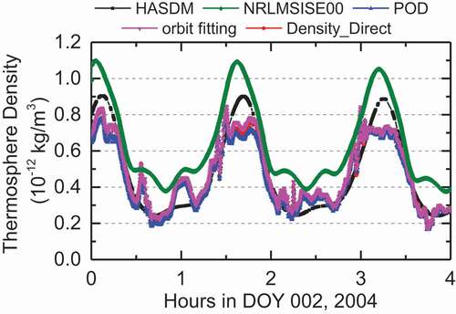
Table 6. Density ratio statistics of NRLMSISE00, HASDM, and Density_Direct over POD and orbit-fitting-derived densities on DOY 002, 2004

Calibration scheme	Mean			STD
	NRLMSISE00	HASDM	Density_Direct	NRLMSISE00	HASDM	Density_Direct
POD	1.522	1.115	1.047	0.256	0.206	0.047
Orbit fitting	1.474	1.078	1.013	0.273	0.212	0.067

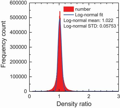
We compared all the POD and orbit-fitting-derived densities from 2004 to 2007 and obtained over 800 million density ratios. A log-normal distribution is applied to fit the density ratios to analyze the differences between these two density data sets. The frequency counts of the density ratios as well as the results of log-normal distribution fitting are illustrated in Figure 9. The two density data sets agree with each other with a very high correlation coefficient of 0.9976. A small bias of 2.20% is found between the orbit-fitting and POD densities and their log-normal STD is 5.75%. These figures are obviously larger than the Bx differences given in Table 5, which should be attributed to the fact that the accelerometer-derived densities are not linearly related to the calibration parameters.

Figure 9. Frequency count of density ratios of orbit fitting over POD densities and its log-normal distribution fit. The bin interval for the frequency count is 0.01.

All the densities during 2004 and 2007 from POD and orbit-fitting schemes are compared to NRLMSISE00, HASDM, and Density_Direct for the precision evaluation. The log-normal distribution fit is applied to their density ratios; the fitting mean and STD values are listed in Table 7. In general, the thermosphere densities generated by orbit fitting and POD are at very similar precision level, and they indicate very similar statistics when compared to the empirical models as well as the accelerometer-based densities. The NRLMSISE00 model indicates a bias of 33.7% and an STD of 0.262 with respect to the POD densities, as well as a bias of 29.9% and an STD of 27.2% with respect to the orbit-fitting densities. For HASDM, the bias is improved to 8.8% and 5.9% while the STD is reduced to 20.5% and 21.0% compared to the POD and orbit-fitting results, respectively. The density differences between POD, orbit fitting, and Density_Direct are the best among others. The bias and STD values between POD and Density_Direct are 1.6% and 5.7%, respectively, while those between orbit fitting and Density_Direct are −0.1% and 5.6%.

Table 7. Log-normal distribution fit to density ratios of NRLMSISE00, HASDM, and Density_Direct to POD and orbit-fitting densities (all the density results during 2004 and 2007 are considered)

Calibration scheme	Log-normal distribution fit mean			Log-normal distribution fit STD
	NRLMSISE00	HASDM	Density_Direct	NRLMSISE00	HASDM	Density_Direct
POD	1.337	1.088	1.016	0.262	0.205	0.057
Orbit fitting	1.299	1.059	0.990	0.272	0.210	0.056

7. Conclusion

In this study, the GRACE on-board accelerometer calibration is investigated using the dynamic calibration method. Two different methods are implemented and compared. The first method is to estimate the calibration parameters during a POD procedure that combines the on-board GPS data, while the second during an orbit-fitting process that requires kinematic orbits. To confirm and validate the proposed calibration schemes, the GRACE data during 2004 and 2007 is analyzed.

The GRACE accelerometer calibration is investigated focusing on its parametrization. The scale coefficients of GRACE accelerometer are fixed to their a priori values while the bias parameters are estimated using piecewise-constant model. Different bias estimation intervals are tested in this study to optimize the orbit fit and orbit determination precision. The results indicate that estimating the bias parameters every 60 min can achieve orbit precision at 2 cm level, as confirmed by orbit comparison to the JPL PSOs as well as the SLR fitting residuals. With this processing strategy, the integrity of the accelerometer biases is preserved since no extra empirical dynamical compensations are estimated during the calibration. The estimated biases from the POD and orbit-fitting schemes show good agreement in the SBF-X and SBF-Y components with differences of −0.04% ± 0.26% and 0.00% ± 0.11%, respectively, while there is a systematic offset in the SBF-Z component at about −7.25% ± 3.85%.

We derived the densities from GRACE-A satellite accelerometer data using the Bx parameters from orbit-fitting and POD schemes, respectively. The density differences between these two schemes are very small and are only at 2.2%±5.75% level. The derived densities are also confirmed by comparison to empirical models such as NRLMSISE00 and HASDM as well as the accelerometer-based density products published by Doornbos (2012), finding that the differences are 1.6%±5.7% and −0.1%±5.6% for the POD and orbit-fitting schemes, respectively. The density comparison of POD and orbit fitting over the NRLMSISE00 model reveals that the NRLMSISE00 exhibits a bias about 30% and a STD about 27% during 2004 and 2007 at the altitude of GRACE satellite, while that over the HASDM gives an improved bias at 7% level and a reduced STD at 21% level.

Considering the increasing LEO-based accelerometer measurements from the ongoing SWARM and GRACE follow-on missions, the efficiency in accelerometer calibration can be very critical in deriving the thermosphere density. The orbit-fitting scheme proposed in our study can avoid the complexity in processing the onboard GPS data and more importantly it can deliver calibration precision at similar level with respect to the POD scheme. Thus, it is very suitable in thermosphere density derivation from on-board accelerometers.

Acknowledgments

We would like to acknowledge the ISDC for providing the GRACE data, JPL for providing the JPL precision products, and Dr. Doornbos for providing the GRACE density products.

Disclosure statement

No potential conflict of interest was reported by the author(s).

Data availability statement

All data included in this research are available upon request by contacting with the corresponding author by [email protected].

Additional information

Funding

This research is sponsored by the National Natural Science Foundation [grant numbers 42004020, 42074032, 41931075 and 42030109]; National Defense Key Laboratory of Aerospace Flight Dynamics technology (grant number 6142210190101); China Postdoctoral Science Foundation [grant number 2021M692460]; the Fundamental Research Funds for the Central Universities [grant number 2042021kf0060]; and Wuhan Science and Technology Bureau [grant number 2019010701011391].

Notes on contributors

Min Li

Min Li is a professor in GNSS Research Center, Wuhan University. He received the B.S. and Ph.D. degrees in geodesy and surveying engineering from Wuhan University in 2005 and 2011, respectively. His research interests include GNSS/LEO satellite precise orbit determination as well as multi-GNSS processing using GPS, GLONASS, BeiDou, and Galileo.

Zhuo Lei

Zhuo Lei is currently a master candidate at the Wuhan University. She has completed her B.Sc. at the College of Geology Engineering and Geomatics, Chang’an University, in 2019. Her area of research currently focuses on the GNSS data processing.

Wenwen Li

Wenwen Li is a research assistant in GNSS Research Center, Wuhan University. He received his B.S., M.S., and Ph.D. degrees from Wuhan University in 2012, 2015, and 2019, respectively. His current research focuses on LEO-based GNSS data precise processing and its application in atmosphere studies including thermosphere and ionosphere inversion.

Kecai Jiang

Kecai Jiang received the B.S. degree in geomatics engineering from Central South University in 2013, and the Ph.D. degree in geodesy and surveying engineering from Wuhan University in 2020. He is currently a Postdoctoral Researcher with Wuhan University. His current research mainly focuses on LEO orbit determination using GNSS.

Youcun Wang

Youcun Wang received the M.S. degree in geomatics engineering from the Shandong University of Science and Technology in 2019. He is currently working toward the doctoral degree in geodesy and surveying engineering at Wuhan University. His main research interests include the precision orbit determination of LEO and dynamics model refinement.

Qile Zhao

Qile Zhao is a professor in GNSS Research Center, Wuhan University. He received the Ph.D. degree in geodesy and surveying engineering from Wuhan University in 2004. His current research interests are precise orbit determination of GNSS and LEO satellites, and high-precision positioning using GPS, Galileo, and BeiDou system.

References

- Bettadpur, S. 2003. Recommendation for A-priori Bias & Scale Parameters for Level-1B ACC Data (Release 00), GRACE TN-04-02. Austin: Center for Space Research, The University of Texas.
- Bettadpur, S. 2012. GRACE Product Specification Document. Austin: Center for Space Research, The University of Texas.
- Bezděk, A. 2010. “Calibration of Accelerometers aboard GRACE Satellites by Comparison with POD-based Nongravitational Accelerations.” Journal of Geodynamics 50 (5): 410–423. doi:https://doi.org/10.1016/j.jog.2010.05.001.
- Bhanderi, D., and T. Bak. 2005. ”Modeling earth albedo for satellites in earth orbit”. Paper presented at the AIAA Guidance, Navigation, and Control Conference and Exhibit, San Francisco, USA.
- Bowman, B.R., and M.F. Storz. 2003. “High Accuracy Satellite Drag Model (HASDM) Review.” Advances in the Astronautical Sciences 116: 1943–1952.
- Bruinsma, S., D. Tamagnan, and R. Biancale. 2004. “Atmospheric Densities Derived from CHAMP/STAR Accelerometer Observations.” Planetary and Space Science 52 (4): 297–312. doi:https://doi.org/10.1016/j.pss.2003.11.004.
- Bruinsma, S., J.M. Forbes, R.S. Nerem, and X. Zhang. 2006. “Thermosphere Density Response to the 20–21 November 2003 Solar and Geomagnetic Storm from CHAMP and GRACE Accelerometer Data.” Journal of Geophysical Research: Space Physics 111 (A6). doi:https://doi.org/10.1029/2005JA011284.
- Bruinsma, S., R. Biancale, and F. Perosanz. 2007. “Calibration Parameters of the CHAMP and GRACE Accelerometers.” In IUGG XXIV General Assembly, Perugia.
- Bruinsma, S., S. Loyer, J.M. Lemoine, F. Perosanz, and D. Tamagnan. 2003. “The Impact of Accelerometry on CHAMP Orbit Determination.” Journal of Geodesy 77 (1–2): 86–93. doi:https://doi.org/10.1007/s00190-002-0304-3.
- Case, K., G. Kruizinga, and S. Wu. 2010. GRACE Level 1B Data Product User Handbook. Pasadena: JPL Publication D-22027.
- Chen, J.L., C.R. Wilson, J.S. Famiglietti, and M. Rodell. 2005. “Spatial Sensitivity of the Gravity Recovery And Climate Experiment (GRACE) Time-variable Gravity Observations.” Journal of Geophysical Research: Solid Earth 110 (B8). doi:https://doi.org/10.1029/2004JB003536.
- Dahle, C., F. Flechtner, C. Gruber, D. König, R. König, G. Michalak, K.-H. Neumayer, and Deutsches GeoForschungsZentrum GFZ. 2013. GFZ GRACE Level-2 Processing Standards Document for Level-2 Product Release 0005. Potsdam: Deutsches GeoForschungsZentrum GFZ.
- Desai, S., W.I. Bertiger, M. Garcia Fernandez, B.J. Haines, C. Selle, A. Sibois, A. Sibthorpe, and J.P. Weiss. 2014. “JPL’s Reanalysis of Historical GPS Data for the Second IGS Reanalysis Campaign.” Paper presented at the AGU Fall Meeting Abstracts, San Francisco, USA.
- Doornbos, E., J. van den Ijssel, H. Luhr, M. Forster, and G. Koppenwallner. 2012. “Neutral Density and Crosswind Determination from Arbitrarily Oriented Multiaxis Accelerometers on Satellites.” Journal of Spacecraft and Rockets 47 (4): 580–589. doi:https://doi.org/10.2514/1.48114.
- Doornbos, E. 2012. Thermospheric Density and Wind Determination from Satellite Dynamics. Berlin, Heidelberg: Springer Science & Business Media.
- Drob, D.P., J.T. Emmert, G. Crowley, J.M. Picone, G.G. Shepherd, W. Skinner, P. Hays, R.J. Niciejewski, M. Larsen, and C.Y. She. 2008. “An Empirical Model of the Earth’s Horizontal Wind Fields: HWM07.” Journal of Geophysical Research Space Physics 113 (A12): 18. doi:https://doi.org/10.1029/2008JA013668.
- Flury, J., S. Bettadpur, and B.D. Tapley. 2008. “Precise Accelerometry Onboard the GRACE Gravity Field Satellite Mission.” Advances in Space Research 42 (8): 1414–1423. doi:https://doi.org/10.1016/j.asr.2008.05.004.
- Foerste, C., R. Shako, F. Flechtner, C. Dahle, O. Abrikosov, H. Neumayer, F. Barthelmes, S.L. Bruinsma, J. Marty, and G. Balmino. 2011. “A New Combined Global Gravity Field Model Including GOCE Data from the Collaboration of GFZ Potsdam and GRGS Toulouse.” Paper presented at the AGU Fall Meeting Abstracts, San Francisco, California.
- Frommknecht, B. 2007. Integrated Sensor Analysis of the GRACE Mission. München: Technische Universität München.
- Gerlach, C., L. Földvary, D. Švehla, T. Gruber, M. Wermuth, N. Sneeuw, B. Frommknecht, et al. 2003. “A CHAMP-only Gravity Field Model from Kinematic Orbits Using the Energy Integral.” Geophysical Research Letters 30 (20): 2037. doi:https://doi.org/10.1029/2003GL018025.
- Guo, X., Q. Zhao, P. Ditmar, Y. Sun, and J. Liu. 2018. “Improvements in the Monthly Gravity Field Solutions through Modeling the Colored Noise in the GRACE Data.” Journal of Geophysical Research: Solid Earth 123 (8): 7040–7054. doi:https://doi.org/10.1029/2018JB015601.
- Jäggi, A., U. Hugentobler, H. Bock, and G. Beutler. 2007. “Precise Orbit Determination for GRACE Using Undifferenced or Doubly Differenced GPS Data.” Advances in Space Research 39 (10): 1612–1619. doi:https://doi.org/10.1016/j.asr.2007.03.012.
- Jin, S., A. Calabia, and L. Yuan. 2018. “Thermospheric Variations from GNSS and Accelerometer Measurements on Small Satellites.” Proceedings of the IEEE 106 (3): 484–495. doi:https://doi.org/10.1109/JPROC.2018.2796084.
- Kang, Z., B. Tapley, S. Bettadpur, J. Ries, P. Nagel, and R. Pastor. 2006. “Precise Orbit Determination for the GRACE Mission Using Only GPS Data.” Journal of Geodesy 80 (6): 322–331. doi:https://doi.org/10.1007/s00190-006-0073-5.
- Klinger, B., and T. Mayer-Gürr. 2016. “The Role of Accelerometer Data Calibration within GRACE Gravity Field Recovery: Results from ITSG-Grace2016.” Advances in Space Research 58 (9): 1597–1609. doi:https://doi.org/10.1016/j.asr.2016.08.007.
- Koch, I., A. Shabanloui, and J. Flury. 2019. “Calibration of GRACE Accelerometers Using Two Types of Reference Accelerations.” Paper presented at the International Symposium on Advancing Geodesy in a Changing World, Cham.
- Liu, J., and M. Ge. 2003. “PANDA Software and Its Preliminary Result of Positioning and Orbit Determination.” Wuhan University Journal of Natural Sciences 8 (2): 603–609. doi:https://doi.org/10.1007/BF02899825.
- Lyard, F., F. Lefevre, T. Letellier, and O. Francis. 2006. “Modelling the Global Ocean Tides: Modern Insights from FES2004.” Ocean Dynamics 56 (5): 394–415. doi:https://doi.org/10.1007/s10236-006-0086-x.
- Marcos, F.A., B.R. Bowman, and R.E. Sheehan. 2006. “Accuracy of Earth’s Thermospheric Neutral Density Models.” Paper presented at the AIAA/AAS Astrodynamics Specialist Conference and Exhibit, Keystone, CO.
- McCarthy, D.D., and G. Petit. 2004. IERS Conventions (2003). Germany: International Earth Rotation And Reference Systems Service (IERS).
- Montenbruck, O., and E. Gill. 2000. Satellite Orbits: Models, Methods, and Applications. Berlin, Heidelberg: Springer Science & Business Media.
- Montenbruck, O., S. Hackel, J. van den Ijssel, and D. Arnold. 2018. “Reduced Dynamic and Kinematic Precise Orbit Determination for the Swarm Mission from 4 Years of GPS Tracking.” GPS Solutions 22 (3): 79. doi:https://doi.org/10.1007/s10291-018-0746-6.
- Picone, J.M., A.E. Hedin, D.P. Drob, and A.C. Aikin. 2002. “NRLMSISE‐00 Empirical Model of the Atmosphere: Statistical Comparisons and Scientific Issues.” Journal of Geophysical Research: Space Physics (1978–2012) 107 (A12): SIA15-1-SIA-6. doi:https://doi.org/10.1029/2002JA009430.
- Reigber, C., G. Balmino, P. Schwintzer, R. Biancale, A. Bode, J.M. Lemoine, R. König, et al. 2002. “A High-quality Global Gravity Field Model from CHAMP GPS Tracking Data and Accelerometry (EIGEN-1S).” Geophysical Research Letters 29 (14): 1692. doi:https://doi.org/10.1029/2002GL015064.
- Schmid, R., M. Rothacher, D. Thaller, and P. Steigenberger. 2005. “Absolute Phase Center Corrections of Satellite and Receiver Antennas.” GPS Solutions 9 (4): 283–293. doi:https://doi.org/10.1007/s10291-005-0134-x.
- Storz, M.F., B.R. Bowman, M.J.I. Branson, S.J. Casali, and W.K. Tobiska. 2005. “High Accuracy Satellite Drag Model (HASDM).” Advances in Space Research 36 (12): 2497–2505. doi:https://doi.org/10.1016/j.asr.2004.02.020.
- Sutton, E.K., J.M. Forbes, and R.S. Nerem. 2005. “Global Thermospheric Neutral Density and Wind Response to the Severe 2003 Geomagnetic Storms from CHAMP Accelerometer Data.” Journal of Geophysical Research: Space Physics 110 (A9): A09S40. doi:https://doi.org/10.1029/2004ja010985.
- Sutton, E.K., R.S. Nerem, and J.M. Forbes. 2007. “Density and Winds in the Thermosphere Deduced from Accelerometer Data.” Journal of Spacecraft and Rockets 44 (6): 1210–1219. doi:https://doi.org/10.2514/1.28641.
- Van Helleputte, T., E. Doornbos, and P. Visser. 2009. “CHAMP and GRACE Accelerometer Calibration by GPS-based Orbit Determination.” Advances in Space Research 43 (12): 1890–1896. doi:https://doi.org/10.1016/j.asr.2009.02.017.
- Van Helleputte, T., and P. Visser. 2008. “GPS Based Orbit Determination Using Accelerometer Data.” Aerospace Science and Technology 12 (6): 478–484. doi:https://doi.org/10.1016/j.ast.2007.11.002.
- Vielberg, K., E. Forootan, C. Lück, A. Löcher, J. Kusche, and B. Klaus. 2018. “Comparison of Accelerometer Data Calibration Methods Used in Thermospheric Neutral Density Estimation.” Annales Geophysicae 36 (3): 761–779. doi:https://doi.org/10.5194/angeo-36-761-2018.
- Visser, P.N.A.M., and J.A.A. Vanden Ijssel. 2016. “Calibration and Validation of Individual GOCE Accelerometers by Precise Orbit Determination.” Journal of Geodesy 90 (1): 1–13. doi:https://doi.org/10.1007/s00190-015-0850-0.
- Wöske, F., T. Kato, B. Rievers, and M. List. 2019. “GRACE Accelerometer Calibration by High Precision Non-gravitational Force Modeling.” Advances in Space Research 63 (3): 1318–1335. doi:https://doi.org/10.1016/j.asr.2018.10.025.
- Zehentner, N., and T. Mayer-Gürr. 2015. “Precise Orbit Determination Based on Raw GPS Measurements.” Journal of Geodesy 1–12. doi:https://doi.org/10.1007/s00190-015-0872-7.