Evaluation of wave retrieval for Chinese Gaofen-3 synthetic aperture radar

ABSTRACT

The goal of this study was to investigate the performance of a spectral-transformation wave retrieval algorithm and confirm the accuracy of wave retrieval from C-band Chinese Gaofen-3 (GF-3) Synthetic Aperture Radar (SAR) images. More than 200 GF-3 SAR images of the coastal China Sea and the Japan Sea for dates from January to July 2020 were acquired in the Quad-Polarization Strip (QPS) mode. The images had a swath of 30 km and a spatial resolution of 8 m pixel size. They were processed to retrieve Significant Wave Height (SWH), which is simulated from a numerical wave model called Simulating WAves Nearshore (SWAN). The first-guess spectrum is essential to the accuracy of Synthetic Aperture Radar (SAR) wave spectrum retrieval. Therefore, we proposed a wave retrieval scheme combining the theocratic-based Max Planck Institute Algorithm (MPI), a Semi-Parametric Retrieval Algorithm (SPRA), and the Parameterized First-guess Spectrum Method (PFSM), in which a full wave-number spectrum and a non-empirical ocean spectrum proposed by Elfouhaily are applied. The PFSM can be driven using the wind speed without calculating the dominant wave phase speed. Wind speeds were retrieved using a Vertical-Vertical (VV) polarized geophysical model function C-SARMOD2. The proposed algorithm was implemented for all collected SAR images. A comparison of SAR-derived wind speeds with European Center for Medium-Range Weather Forecasts (ECMWF) ERA-5 data showed a 1.95 m/s Root-Mean-Squared Error (RMSE). The comparison of retrieved SWH with SWAN-simulated results demonstrated a 0.47 m RMSE, which is less than the 0.68 m RMSE of SWH when using the PFSM algorithm.

KEYWORDS:

• Wave retrieval
• Gaofen-3 (GF-3)
• Synthetic Aperture Radar (SAR)

1. Introduction

Offshore regions are important areas for human activities. The coastal seas are also complex regions with various ocean dynamics, e.g. wave breaking, upwelling, ocean fronts, and mesoscale eddies. Traditionally, the measurements in these regions are mainly conducted using station-based, ship-based, and satellite observations. Numericall wave models, such as the third-generation Simulating WAves Nearshore (SWAN) (Siadatmousavi and Jose 2010; Ou et al. 2002; Booij, Ris, and Holthuijsen 1999; SWAN Team 2019, developed at Delft University of Technology) and WAVEWATCH-III (WW3) (Tolman 2014; Hu et al. 2020), are important methods for hindcasting waves. Although these methods achieve high accuracy in long-term comparisons, the prediction accuracy of wave modeling is reduced when simulating individual events due to driving wind fields and boundary conditions. Satellite altimetry (Foreman, Holt, and Kelsall 1994) and scatterometry (Tsai et al. 2000) are commonly used for wave and wind monitoring of coastal waters. However, these satellite-based data have limits when measuring ocean wave parameters over a wide range, i.e. 10 km spatial coverage for the altimeter and 12.5 km for the scatterometer. Synthetic Aperture Radar (SAR) is a useful technique for marine monitoring, having a wide spatial coverage and fine resolution. Chinese Gaofen-3 (GF-3) SAR images acquired in Fine Spotlight (FS) or Quad-Polarization Strip-I (QPS-I) modes have a pixel size of 1 m (FS) to 8 m (QPS-I) and a spatial coverage of 10 km (FS) to 30 km (QPS-I) (Shao et al. 2019; Zhu et al. 2019a).

Methodologies for wind (Alpers and Brummer 1994) and wave retrieval from SAR images have been well studied over the past decades. In the literature, the Geophysical Model Function (GMF), describing the microwave backscattered signal and sea surface state (Masuko et al. 1986), has been successfully developed for inverting wind speed when using the prior wind direction (Chapron, Johnsen, and Garello 2001). The copolarization (Vertical-Vertical (VV) and Horizontal-Horizontal (HH)) wind speed inversion GMFs include CMOD7 stored as a look-up table (Stoffelen et al. 2017) and C-SARMOD2 (Lu et al. 2018) at C-band, XMOD2 (Li and Lehner 2013) at X-band, and LMOD at L-band (Isoguchi and Shimada 2009). These data are directly derived from global SAR-measured Normalized Radar Cross-Section (NRCS) and independent wind data from buoys, scatterometers, and European Center for Medium-Range Weather Forecasts (ECMWF). Validation of the estimated wind speed from SAR images showed about 2 m/s Root Mean Square Error (RMSE) for open seas (Shao, Shen, and Sun 2017a). However, retrieved wind speed had a larger deviation in coastal waters in the presence of upwelling (Li, Li, and He 2009). GMFs have been developed for strong winds from typhoons and hurricanes, using the cross-polarization of RADARSAT-2 (R-2) (Zhang and Perrie 2012), Sentinel-1 (S-1) (Gao et al. 2018, 2020), and GF-3 SAR images (Shao et al. 2018). The accuracy of low-to-moderate wind speeds derived from cross-polarized SAR is affected by the low signal-to-noise ratio. Strong winds can also be retrieved using SAR-derived ocean wave parameters (Shao et al. 2017b; Hwang, Li, and Zhang 2017; Shao et al. 2020a).

The ocean wave mapping mechanism on SAR has been studied since the 1980s. Three modulations that contribute to the mechanism have been found: tilt modulation (Engen et al. 2000), hydrodynamic modulation, and the unique transformation velocity bunching (Alpers and Bruning 1986; Alpers, Ross, and Rufenach 1981). A theocratic-based wave retrieval algorithm for copolarization SAR, called the Max Planck Institute Algorithm (MPI), was developed in 1991 (Hasselmann and Hasselmann 1991) and later improved (Hasselmann, Bruning, and Hasselmann 1996). The principle of the MPI algorithm is to minimize the simulated SAR intensity spectrum using the Modulation Transfer Function (MTF) of each SAR mapping modulation and observed SAR intensity spectrum. The MTF converts the image spectrum into a wave spectrum with a subsequent estimation of the integrated sea state parameters (Lyzenga 1986). Due to the nonlinearity of the MTF of velocity bunching in the flight direction (Stopa et al. 2016), a first-guess wave spectrum is necessary. Instead of using the simulated wave spectrum from a numerical wave model, the SemiParametric Retrieval Algorithm (SPRA) (Mastenbroek and de Valk 2000) takes advantage of the empirical parametric JONSWAP wave spectrum (Hasselmann, Dunckel, and Ewing 1980) to produce a first-guess wave spectrum. The PArtition Rescaling and Shift Algorithm (PARSA) (Schulz-Stellenfleth, Lehner, and Hoja 2005; Li et al. 2010) and the Parameterized First-guess Spectrum Method (PFSM) (Sun and Guan 2006; Lin et al. 2017) also follow the MPI scheme. The cross-polarized SAR spectrum is used as an input to the PARSA algorithm to resolve the 180° ambiguity of the wave propagation direction. The model-induced error of the swell SAR spectrum is improved with the PFSM algorithm. Recently, efforts have been made to enhance the wave retrieval algorithm using Quad-Polarization (Q-P) SAR images (He, Shen, and Perrie 2006) and a SAR-derived wave slope spectrum. An analysis of Significant Wave Height (SWH) retrieved from GF-3 SAR images acquired in the wave mode revealed that Q-P encounters the saturation problem at SWH up to 1.4 m (Zhu et al. 2019b). This may be caused by the low signal-to-noise ratio at cross-polarization. As the MTFs of mapping modulations are complex, empirical models have also been designed for calculating each MTF in the retrieval scheme, e.g. CWAVE (Schulz-Stellenfleth, Konig, and Lehner 2007; Stopa and Mouche 2016), XWAVE (Li, Lehner, and Bruns 2011; Bruck and Lehner 2013; Pleskachevsky, Rosenthal, and Lehner 2016), and CSAR_WAVE (Sheng et al. 2018). These MTFs estimate the sea state parameters directly from SAR features derived from the scene, including an image spectrum without spectral transformation. Both methods have advantages and disadvantages. The spectral transformations only work in the regions where the wave patterns are unambiguously imaged. For instance, only around 30% of all acquisitions can be applied using the spectral-transformation method for Sentinel-1 interferometric wide swath mode (200 km coverage with 10 m pixel), whereas with empirical functions, almost 99% of acquisitions are applicable (Pleskachevsky et al. 2019). However, using empirical functions does not provide a wave spectrum that can be simply assimilated into a forecast system, although the empirical approach does allow for rapid and robust processing of SAR scenes in near real-time. Due to the dramatic variations in water depth found in coastal areas, the wind–sea and wind–swell systems mix, and empirical algorithms must be refitted to provide more accurate results under various marine phenomena conditions. The usability of the first-guess wave spectrum also affects the accuracy of SAR wave inversion. The wave spectrum proposed by Elfouhaily, Chapron, and Katsaros (1997), denoted as E-spectrum, is a full wave-number spectrum derived from classic ocean wave models, e.g. JONSWAP and PM (Pierson and Moskowitz 1963). Therefore, in our work, we implemented a combined wave retrieval scheme of MPI, SPRA, and PFSM for GF-3 SAR images for coastal China Seas and the Japan Sea. The E-spectrum is applied in this scheme.

The remainder of this paper is organized as follows. Section 2 presents the GF-3 SAR images, the ECMWF data, the measurements from the Jason-3 altimeter, and the settings of the SWAN model. The scheme of the SAR wave retrieval is presented in Section 3. Comparisons of SWH retrieval are described in Section 4. The conclusions are summarized in Section 5.

2. Dataset

2.1. SAR data

For this study, we used more than 200 GF-3 SAR images obtained from an official platform provided by the National Satellite Ocean Application Service (NSOAS). The imagery covered the coastal China Seas and the Japan Sea from January to July 2020. These images were acquired in the QPS-I mode as a Level-1 (L-1) product. The following equation was used for calibration:

(1) ${\sigma }^0=\mathit{D}{N}^2{\left(\frac{M}{C}\right)}^2-\mathit{N}[\mathit{dB}]$(1)

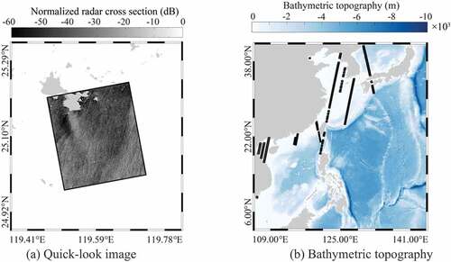
where C is a constant (=32767), M and N are quantitative constants available in the file accompanying the SAR intensity data DN, and ${\sigma }^0$ is the NRCS united in dB. The range incidence angle is between 21° and 50°. The GF-3 SAR scenes were divided into 128 × 128 pixel sub-scenes with that is the spatial coverage applied Fast Fourier Transform (FFT) method is ~1 km at horizontal direction due to the pixel resolution is 8 m. For example, Figure 1(a) shows the quick-look image after calibrating the VV-polarized SAR image taken on 21 January 2020 at 10:11 UTC, which was acquired from the coastal waters of the East China Sea. The information from collected GF-3 SAR images is illustrated in Figure 1(b), in which the rectangles represent the spatial coverage.

Figure 1. (a) Calibrated vertical-vertical (VV) polarization quick-look image of Gaofen-3 (GF-3) Synthetic Aperture Radar (SAR) image captured on 21 January 2020 at 10:11 UTC in the coastal waters of the East China Sea. (b) Information on GF-3 SAR images collected from January to July 2020, in which the rectangles represent the spatial coverage.

2.2. Hindcast data

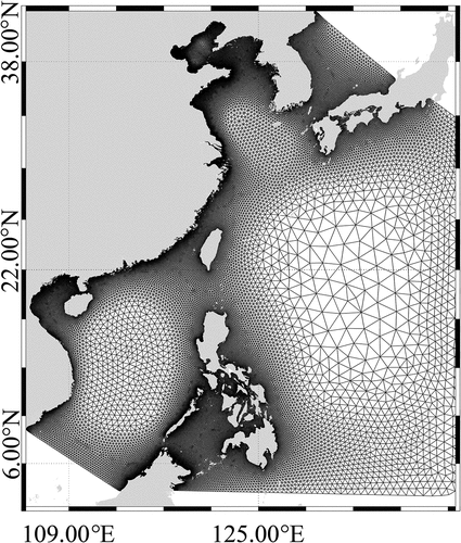
Observations from moored buoys are recognized as the most accurate method for measuring sea surface dynamics. As there are no such buoys in the coastal China Seas, a third-generation numeric model, the SWAN model, was used for simulating wave fields (Yang et al. 2020). In regions with complex coastlines, the unstructured grids of the SWAN model mean that it performs better than the WW3 model with its rectangle grids. Unstructured grids are most suitable for the complicated and changing wave phenomena encountered offshore, e.g. depth-induced wave breaking and stationary wave. In this study, the modeling duration of the simulated waves in the China Seas and the Japan Sea ranged from 1 December 2019 to 1 July 2020. The modeling region was 19°–38° N and 109°–135° E, as shown in Figure 2. An ECMWF reanalysis of ERA-5 (Hersbach et al. 2018) winds on a 0.5° grid at an interval of 1 h was used as the forcing field. Bathymetric topography with about 1 km of spatial resolution in the horizontal direction was provided by the General Bathymetric Chart of the Oceans (GEBCO) (Weatherall et al. 2015). Sea surface current, sea water elevation, and sea surface temperature on a 0.08° grid at an interval of 3 h were collected from the Hybrid Coordinate Ocean Model (HYCOM) (Shaji et al. 2005) official datasets. Sea surface current and sea water elevation were also used as forcing fields to obtain reliable simulated results for coastal waters where strong tidal currents and water elevations may strongly affect the propagation of waves

Figure 2. Simulated region for the simulating waves nearshore (SWAN) model and the unstructured grid.

.

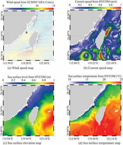
The outputs from SWAN included one-dimensional wave spectra and SWH with a spatial resolution of 1 km and a temporal resolution of 30 min. Note that the time difference between the GF-3 SAR image and the SWAN-simulated waves is less than 15 min. The wind map from ECMWF ERA-5 data for 21 January 2020 at 10:00 UTC is shown in Figure 3(a). The black rectangle represents the spatial coverage of the image in Figure 1(a). Maps of HYCOM sea surface current, sea water elevation, and sea surface temperature on 21 January 2020 at 09:00 UTC are shown in Figure 3(b–d). Table A1 in Appendix A shows the settings of SWAN model in this work.

Figure 3. (a) Wind map from European Center for Medium-Range Weather Forecasts (ECMWF) reanalysis ERA-5 data on 21 January 2020 at 10:00 UTC. (b) Current speed map from the hybrid coordinate ocean model (HYCOM) on 21 January 2020 at 09:00 UTC. (c) Sea surface elevation from HYCOM on 21 January 2020 at 09:00 UTC. (d) Sea surface temperature from HYCOM on 21 January 2020 at 09:00 UTC. Note that the black rectangle represents the spatial coverage of the image in Figure 1(a).

2.3. In situ measurements

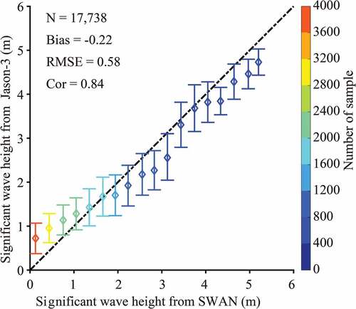
Wave measurements from the Jason-3 altimeter mission have been a valuable source of data for global monitoring (Zhang, Wu, and Chen 2015). Those data are also useful for oceanography research. To confirm the accuracy of SWAN-simulated waves, SWH products for the modeling period were collected from the Jason-3 mission altimeter. Figure 4(a) shows the SWH map overlaid on the SWAN-simulated SWH field for 17:00 UTC on 19 January 2020. The ECMWF wave map is also shown in Figure 4(b). Note that the time difference between SWAN simulations and Jason-3 data is within 15 min. The pattern from the SWAN-simulated SWH field is consistent with the pattern from ECMWF and the Jason-3 altimeter. The SWAN-simulated SWH field was particularly good at replicating details. We also compared the SWAN-simulated SWH with measurements from the Jason-3 altimeter for the period from January to July 2020 (Figure 5). The analysis results indicated a 0.58 m RMSE with a correlation (Cor) of 0.84. In this sense, the SWAN-simulated waves were reliable for this study.

Figure 4. (a) Significant wave height (SWH) map for 17:00 UTC on 19 January 2020. The satellite footprint is shown as colored boxes overlaid on the SWAN-simulated SWH field. (b) Corresponding ECMWF SWH map.

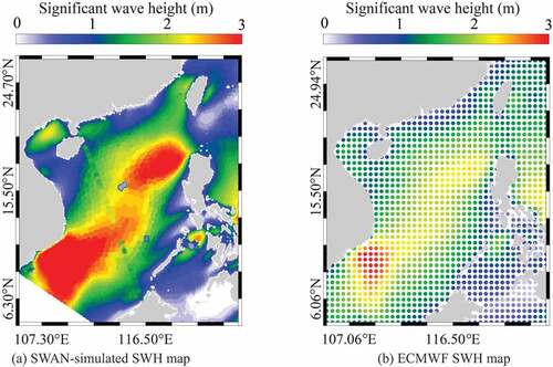
Figure 5. SWAN-simulated SWH compared with the measurements from the Jason-3 altimeter 3 for the period from January to July 2020.

3. Methodology

SAR-derived wind speed is necessary to produce the first-guess wave spectrum in the SAR wave retrieval. Therefore, in this section, the methodology for wind retrieval GMF is introduced, and the wave retrieval algorithm, which is based on the combined scheme of MPI and SPRA, is briefly presented.

3.1. Fractional differential for image enhancement analysis

Although it was originally designed for scatterometry, a well-developed GMF called CMOD4 (Stoffelen and Anderson 1997) has been used for SAR wind retrieval since 1997. Generally, GMF describes an empirical relation between the sea surface wind vector and quantitative NRCS. The updated versions of GMF, CMOD5 (Hersbach, Stoffelen, and Haan 2007), and CMOD5N (Hersbach 2010) improve the performance of GMF at wind speeds up to 33 m/s. The latest CMOD family is GMF C-SARMOD2 and CMOD7, which are derived from SAR-measured NRCS and wind data from moored buoys. The formula for the C-SARMOD2 algorithm is as follows:

(2) $\mathit{z}(\mathit{v},\mathit{f},\mathit{\theta })=B_0^p(U_{10},\mathit{\theta })(1+B_1\left(U_{10},\mathit{\theta }\right)cos\mathit{f}+B_2\left(U_{10},\mathit{\theta }\right)cos2\mathit{f})$(2)

where $\mathit{z}=({\sigma }^0{)}^p$. In this equation, ${\sigma }^0$ is the SAR-measured normalized radar cross-section; p is set to 0.625; U₁₀ is the wind speed at 10-m height; and φ represents the angle between the wind direction and the radar look direction. B₀, B₁, and B₂ are functions of the incidence angle θ and the wind speed at 10 m above the sea surface. A detailed description of the wind retrieval method is provided in Appendix B.

3.2. SAR wave retrieval

As concluded previously (Alpers and Bruning 1986), the unique mapping mechanism velocity bunching between the ocean wave spectrum and the SAR spectrum is a nonlinear modulation. As a result, information smaller than a specific wave number in the azimuth direction is lost due to the relative motion between satellite and waves. This limit is called the cutoff wave number. The simulation experiments also demonstrated that the SAR image spectrum has a 180° direction ambiguity (Hasselmann and Hasselmann 1991). For these reasons, directly solving the inversion from the SAR image spectrum is difficult. The MPI algorithm can be used to retrieve an ocean wave spectrum by constructing a cost function, as described in Equation (4)(4) $T_k^S=4\mathit{i}{k}_r\frac{cot\mathit{\theta }}{1\pm {sin}^2\mathit{\theta }}+4.5\mathit{k\omega }\frac{\mathit{i\mu }-\mathit{\omega }}{{\omega }^2+{\mu }^2}{sin}^2\mathit{\varphi }-\frac{R}{V}{k}_r\mathit{\omega }(cos\mathit{\theta }-\mathit{i}sin\mathit{\theta }\frac{{\mathit{k}}_{\mathit{l}}}{\mathit{k}})$(4) . This requires providing the first-guess wave spectrum.

(3) $\mathit{J}=\int {\left[I_k-{\bar{I}}_{\mathit{k}}\right]}^2\mathit{dk}+\mathit{\mu }\int {\left\{\frac{\left[E_k-{\bar{E}}_{\mathit{k}}\right]}{\left[\mathit{B}+{\bar{E}}_{\mathit{k}}\right]}\right\}}^2\mathit{dk}$(3)

where Ī_k is the first-guess spectrum at wave number k, I_k is the retrieved two-dimensional ocean wave spectrum by minimizing the cost function J, Ē_k is the simulated SAR spectrum using the three MTFs as stated in Equation (5)(5) $k_s={\left(\frac{2.87g{V}^2}{R^2{U}_{10}^4{cos}^2\mathit{\phi }\left({sin}^2\mathit{\phi }{sin}^2\mathit{\theta }+{cos}^2\mathit{\phi }\right)}\right)}^{0.33}$(5) , E_k is the SAR intensity spectrum, μ is the weight coefficient, and the small positive number B is assumed to be 0.001 to ensure convergence is achieved.

(4) $T_k^S=4\mathit{i}{k}_r\frac{cot\mathit{\theta }}{1\pm {sin}^2\mathit{\theta }}+4.5\mathit{k\omega }\frac{\mathit{i\mu }-\mathit{\omega }}{{\omega }^2+{\mu }^2}{sin}^2\mathit{\varphi }-\frac{R}{V}{k}_r\mathit{\omega }(cos\mathit{\theta }-\mathit{i}sin\mathit{\theta }\frac{{\mathit{k}}_{\mathit{l}}}{\mathit{k}})$(4)

where $T_K^S$ is the total SAR MTF, $\mathit{k}$ is the wave number, $k_r$ is the portion wave number at range, $\mathit{\theta }$ is the incidence angle, $\mathit{\varphi }$ is the azimuth angle, $\mathit{\mu }$ is the attenuation factor, $\mathit{\omega }$ is the frequency, R is the SAR irradiation slant distance, V is the satellite movement speed, and k₁ is the portion wave number at azimuth (Lyzenga 1986; Feindt, Schroter, and Alpers 1986; Hasselmann and Hasselmann 1991).

An ocean wave spectrum simulated from a third-generation numerical wave model is used as the first-guess spectrum in the MPI algorithm such as the WAM model (WAMDI Group 1988; Komen et al. 1997). In practice, the SPRA algorithm (Mastenbroek and de Valk 2000) uses a wind–sea spectrum calculated from a parametric function such as JONSWAP. Detailed information on the JONSWAP function can be found in recent research (see appendix in Ding et al. 2019). Similar to the MPI algorithm, this scheme minimizes the cost function. The difference between the simulated SAR spectrum of the retrieved wind-sea spectrum and the observed SAR intensity spectrum might be determined by the swell, in which case velocity bunching can be ignored. However, a wind-sea error is included in the swell SAR retrieval. The PFSM algorithm (Sun and Guan 2006) was developed to improve the model-induced error. Its key feature is that the SAR intensity spectrum is divided into two portions, the wind–sea SAR and the swell SAR, by a separate wave number k_s (Equation 6(6) $B_l=\frac{{\alpha }_p{c}_p}{2\mathit{c}}{F}_p$(6) ). For nonlinear mapping of the wind–sea SAR portion, the parametric JONSWAP wave spectrum is used to produce a best first-guess spectrum by searching for the most suitable parameters, i.e. dominant wave phase velocity and dominate wave direction. Next, the scheme of the algorithm is used to retrieve the wind–sea spectrum. The swell spectrum is directly inverted by solving the given portion of the SAR spectrum:

(5) $k_s={\left(\frac{2.87g{V}^2}{R^2{U}_{10}^4{cos}^2\mathit{\phi }\left({sin}^2\mathit{\phi }{sin}^2\mathit{\theta }+{cos}^2\mathit{\phi }\right)}\right)}^{0.33}$(5)

where gravitational acceleration g is constant at 9.8 m/s², V is a flight velocity of 7600 m/s for GF-3 SAR satellite, R is the satellite slant range, U₁₀ is the SAR-derived wind speed, θ is the radar incidence angle, and φ is the angle of the wave propagation direction relative to the radar look direction.

The PFSM algorithm has rarely been applied to wave retrieval from SAR images of coastal waters because the JONSWAP wave spectrum is more suitable for wind–sea interactions. A universally applicable spectral model was proposed, in which the key factor is the synthesized spectrum based on the high (Phillips 1985) and low wave number regimes (Hwang, Atakturk, and Sletten 1996).

The low wave-number and high spectrum of the E-spectrum follow these equations:

(6) $B_l=\frac{{\alpha }_p{c}_p}{2\mathit{c}}{F}_p$(6)

(7) $B_h=\frac{{\alpha }_m{c}_m}{2\mathit{c}}{F}_m$(7)

where

(8) ${\alpha }_p=0.006{\mathrm{\Omega }}^{0.5}$(8)

where Ω (=U₁₀/c_p) is the dimensionless wave age, U₁₀ is the wind speed at 10-m height, c is the phase velocity, c_p is the dominant wave phase velocity, F_p is the long-wave-induced effect function, α_m represents the equilibrium range parameter for short waves, c_m is the minimum wave phase velocity treated as a constant (0.23), and F_m is the short-wave-induced effect function. The two-dimensional wave spectrum S(k,ϕ) of the E-spectrum model in terms of wave number k and direction ϕ is the one-dimensional wave spectrum multiplied by the directional function G(k,ϕ), expressed as follows:

(9) $\mathit{S}(\mathit{k},\mathit{\varphi })={\mathrm{\Omega }}^{-3}(B_l+B_h)\mathit{G}(\mathit{k},\mathit{\varphi })$(9)

where

(10) $\mathit{G}(\mathit{k},\mathit{\varphi })=\frac{1}{2\mathit{\pi k}}[1+\mathrm{\Delta }(\mathit{k})cos2\mathit{\varphi }]$(10)

(11) $\mathrm{\Delta }(\mathit{k})=tanh[a_0+a_p(\frac{c}{c_p}{)}^{2.5}+a_m(\frac{c}{c_m}{)}^{2.5}]$(11)

where a₀ is taken to be 0.1733, a_p is the constant of 4, a_m = 0.13 u*/c_m, and u* is assumed to be the friction wind speed, which can be calculated from the following functions (Maat, Kraan, and Oost 1991):

(12) $u^{\ast }=(0.4c_p{z}_0\mathit{g}{)}^{-3}$(12)

(13) $z_0=0.000037\frac{U_{10}^2}{\mathit{g}}(\frac{{\mathit{U}}_{10}}{c_p}{)}^{0.9}$(13)

The dominant phase speed or the cutoff wavelength derived from the SAR intensity spectrum is strongly affected by the nonlinearity caused by velocity bunching on SAR in the presence of complicated marine phenomena (Shao et al. 2020b). Thus, in this study, we used Equations (7(7) $B_h=\frac{{\alpha }_m{c}_m}{2\mathit{c}}{F}_m$(7) –14(14) $c_p=\frac{{\mathit{U}}_{10}}{11.6\times {(9700\mathit{g})}^{-0.23}}$(14) ) proposed by Elfouhaily, Chapron, and Katsaros (1997) and Donelan, Hamilton, and Hui (1985) to directly obtain the dominant wave phase speed c_p, which is assumed in the calculation from the SAR intensity spectrum:

(14) $c_p=\frac{{\mathit{U}}_{10}}{11.6\times {(9700\mathit{g})}^{-0.23}}$(14)

where U₁₀ is the wind speed at 10 m above the water surface. Under this circumstance, an ocean wave spectrum can easily be produced once the wind speed U₁₀ is known.

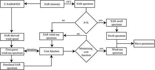
Figure 6 illustrates the one-dimensional spectrum constructed using E-spectrum and the JONSWAP wave spectrum at a wind speed of 8 m/s with the sea fetch of 77,600 m proposed in Elfouhaily, Chapron, and Katsaros (1997). These two models have apparent differences under these conditions. In our work, a wave retrieval scheme combining the MPI, SPRA, and PFSM algorithms was implemented for wave retrieval from a GF-3 SAR image using the SAR-derived wind speed (Rikka et al. 2018). The ocean wave spectrum using the E-spectrum model was taken as the first-guess spectrum. The flowchart is shown in Figure 7.

Figure 6. One-dimensional spectrum using the Elfouhaily (E-spectrum) and JONSWAP wave spectrum at a wind speed of 8 m/s.

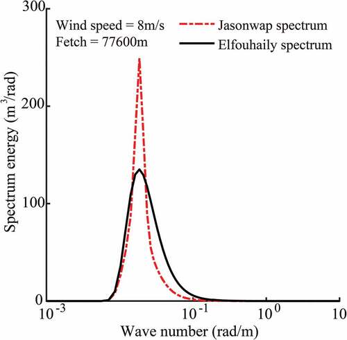
Figure 7. Flowchart of the wave retrieval scheme used in this study.

4. Results and discussions

Initially, we present a case study to illustrate an inverted one-dimensional wave spectrum. The retrieval results are then systematically compared with the SWAN-simulated SWH. Finally, the applicability of the algorithms is analyzed under various conditions, i.e. SAR-derived wind speeds, HYCOM sea surface current, HYCOM sea water elevation, and HYCOM sea surface temperature.

4.1. Results

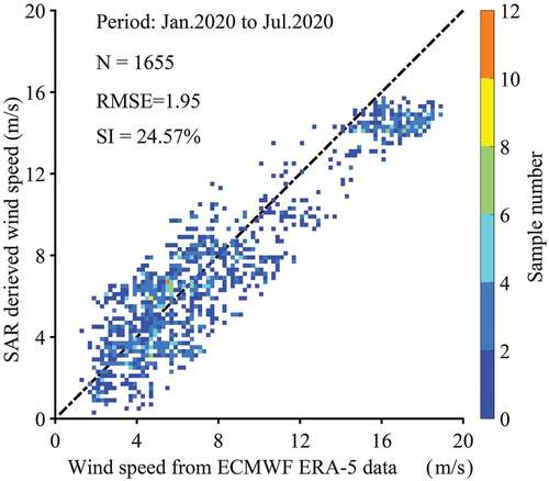
After the ECMWF wind directions were employed, wind speeds at a spatial resolution of 1 km were inverted from the collected GF-3 SAR images. Figure 8 displays the SAR-derived wind map using VV-polarized GMF C-SARMOD2. This figure corresponds to the image in Figure 1(a), in which slow winds with wind speeds less than 5 m/s are probably caused by the Island barrier. The accuracy of wind retrieval from GF-3 SAR images has been well studied (Shao et al. 2019; Shao, Shen, and Sun 2017a) with RMSE values of about 2 m/s reported. Therefore, we simply repeated the validation of the SAR-derived wind speeds against ECMWF winds during the period from January to July 2020, as shown in Figure 9. The color represents the data density in 0.2 m/s bins. The comparison shows a 1.95 m/s RMSE of wind speed, which is closed with the accuracy of wind speed (~2 m/s) for GF-3 SAR. This result indicates that the SAR-derived winds could be used in this context.

Figure 8. SAR-derived wind map using C-SARMOD2 from the GF-3 SAR image taken on 21 January 2020 at 10:11 UTC.

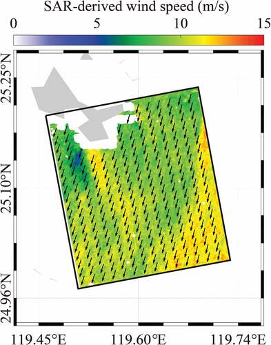
Figure 9. Validation of SAR-derived wind speeds with ECMWF reanalysis (ERA-5) winds for the period from January to July 2020. The color represents the data density in 0.2 m/s bins.

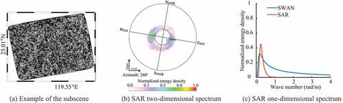
Traditionally, spectral-transformation wave retrieval algorithms work well for a homogenous image with swell waves (Rikka et al. 2018). An example of the subscene in Figure 1(a) covering the SWAN grids is shown in Figure 10(a). In this noisy subscene, the wave pattern is not apparent where wind-sea waves dominate. Additional SAR-derived wind speed data were used when applying the spectral-transformation method. The peak of the corresponding two-dimensional SAR spectrum was also observed, as shown in Figure 10(b). The one-dimensional SAR-derived wave spectrum of the above case is shown in Figure 10(c)

Figure 10. (a) Example of the subscene in Figure 1(a) covering the SWAN grids. (b) Corresponding SAR two-dimensional spectrum. (c) SAR-derived and SWAN-simulated one-dimensional spectrum.

, in which the red line represents the one-dimensional SWAN-simulated wave spectrum. The pattern of the SAR-derived wave spectrum is consistent with that from the SWAN simulation, although the low-frequency portion in the SAR-derived one-dimensional wave spectrum has a cutoff due to velocity bunching. Using the proposed algorithm through the retrieved one-dimensional wave spectrum S(k) as stated in Equation (16), we found that the SAR-derived SWH H_s was 1.98 m, whereas the SWAN-simulated SWH was 2.33 m.

(15) $H_s=4\sqrt{{\int }^S(\mathit{k})\mathit{dk}}$(15)

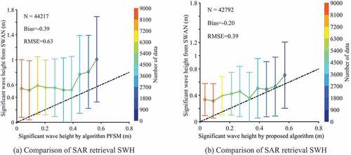
In total, we had more than 10,000 subscenes from the collected SAR images available for evaluating the accuracy of SAR-derived SWH. The PFSM algorithm in which the JONSWAP wave spectrum was employed as the first-guess spectrum was used for wave retrieval. Unfortunately, there were few Jason-3 footprints coinciding with the GF-3 images. The retrieved results were compared statistically with SWAN-simulated SWH. Figure 11(b) reveals a 0.47 m RMSE in SWH using the proposed algorithm. Although some error is acceptable with a 0.68 m RMSE of SWH using the PFSM algorithm, as shown in Figure 11(a), we concluded that the PFSM algorithm performed poorly because the SAR-derived SWH seems to be underestimated at SWH values less than 0.5 m. This was likely caused by inaccurate dominant phase speed for the inhomogeneous SAR images in the inversion scheme. Figure 12 shows the statistical analysis at a low sea state (H_s < 1 m), where short gravity waves dominant. The proposed algorithm yielded a 0.39 RMSE of SWH, which is less than the 0.63 RMSE of SWH by the PFSM algorithm. Due to the weak SAR backscattering signal, it is not surprising that the wave retrieval results had obvious underestimations. However, the proposed algorithm significantly reduced the underestimation of the SAR wave retrieval results. In this case, the proposed algorithm can be operationally applied due to its function only taking the SAR-derived wind speed without calculating the dominant phase speed in the PFSM algorithm.

Figure 11. (a) Comparison between SWAN-simulated SWH and SAR retrieval SWH using the parameterized first-guess spectrum method (PFSM). (b) Comparison between SWAN-simulated SWH and SAR retrieval SWH using the proposed algorithm.

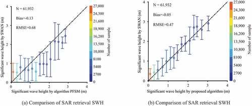
Figure 12. The high frequency radar part results. (a) Comparison between SWAN-simulated SWH and SAR retrieval SWH using the parameterized first-guess spectrum method (PFSM). (b) Comparison between SWAN-simulated SWH and SAR retrieval SWH using the proposed algorithm.

4.2. Discussion

In this section, the applicability of the proposed algorithm is discussed in the context of various sea states. Figure 13(a–d) shows the bias (SAR-derived SWH minus SWAN-simulated SWH) versus several variables, i.e. wind speed, HYCOM sea surface current speed, HYCOM sea water elevation, and HYCOM sea surface temperature. A total of more than 600,000 matchups were divided into groups at a bin size of 1.75 m/s for wind speed, 0.075 m/s for current speed, 0.075 m for sea water elevation, and 1.7°C for sea surface temperature. The error bars represent the standard deviation of each bin

Figure 13. Bias (SAR-derived SWH using the proposed algorithm minus SWAN-simulated SWH) is contrasted with (a) SAR-derived wind speed, (b) sea surface current speed from HYCOM model, (c) sea surface elevation from HYCOM model, and (d) sea surface temperature from HYCOM model.

.

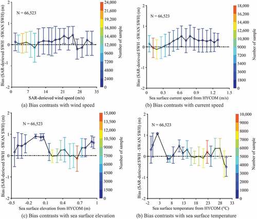
We observed that the relationship between the variation in SWH bias and SAR-derived wind speed was within ±0.3 m, whereas the variation remained about 0.2 m at wind speeds ranging between 10 m/s and 22 m/s. Moreover, the variation in SWH bias remained at about 0.3 m with a current speed greater than 0.3 m/s. This kind of behavior reveals an explicit modulation of wind and current in the SAR wave mapping mechanism. We found that the bias of variation increases up to 1 m at a sea surface elevation of less than 0 m and a sea surface temperature of less than 1°C. We think that upwelling or downwelling dominates under these conditions, causing sea surface convergence and divergence and therefore reducing the accuracy of wave retrieval.

5. Summary

The topic of SAR wave retrieval generally includes the development of algorithms for open seas. However, SAR is also a valuable technique for wave monitoring in coastal waters because it has a higher spatial resolution than buoys and scatterometers. We focused on the applicability of wave retrieval from GF-3 SAR images in the coastal China Seas and the Japan Sea. Inhomogeneous GF-3 SAR images were used for a wave retrieval algorithm. The proposed algorithm takes advantage of the existing theocratic-based algorithms, e.g. MPI, SPRA, and PFSM. A universally applicable spectral model, E-spectrum, was used to produce the first-guess spectrum. This spectrum can be driven using the SAR-derived wind speed without calculating the dominant wave phase speed, which is probably distorted by other marine phenomena.

In total, we had more than 200 recorded VV-polarized GF-3 SAR images acquired in the QPS-I mode collected over the period from November 2019 to July 2020. These cases were divided into subscenes with a spatial resolution of about 1 km², which were matched with SWH from SWAN-simulated waves in 0.1° grids. Validation of the SWAN-simulated SWH against the measurements from the Jason-3 altimeter yielded about 0.6 m RMSE with a 0.84 Cor. The newly released wind retrieval VV-polarized GMF, denoted as C-SARMOD2, was used to retrieve wind speeds from VV-polarized GF-3 SAR images after taking advantage of the ECMWF wind directions. The SAR-derived wind speed was set using prior information in the process of wave retrieval. The analysis showed a 1.95 m/s RMSE of wind speed compared with the wind speed from ECMWF ERA-5 data, which is consistent with the accuracy reported in recent studies.

More than 10,000 scenes were processed using two schemes: the proposed algorithm and the PFSM. The retrieved results were validated against SWAN-simulated SWH from the ECMWF. The validation indicated the RMSE of SWH to be 0.47 when using the proposed algorithm and 0.69 m when using the PFSM. In particular, the proposed algorithm reduced the underestimation of wave retrieval at the low sea state condition. The error of wave retrieval was studied in term of various conditions: SAR-derived wind speed, HYCOM sea surface current, HYCOM sea water elevation, and HYCOM sea surface temperature. The analysis results showed that the variation in SWH bias was about 0.3 m with wind speeds ranging from 10 to 22 m/s and current speeds greater than 0.3 m/s. The sea surface elevation and sea surface temperature have the strongest influence on inversions at sea surface elevations less than 0 m and sea surface temperatures less than 1°C and 0.69°C, where upwelling or downwelling dominates.

In summary, although the proposed algorithm has the potential for use for wave retrieval from GF-3 SAR images that include complicated marine phenomena, the accuracy needs to be improved by considering the effect of sea surface elevation and sea surface temperature. In the future, the sea surface current speed should be retrieved with the GF-3 SAR wave retrieval.

Acknowledgments

We appreciate the National Ocean Satellite Application Center (NSOAS) for sharing the GaoFen-3 (GF-3) SAR images via https://osdds.nsoas.org.cn. The European Centre for Medium-Range Weather Forecasts (ECMWF) data were accessed via http://www.ecmwf.int. The Operational Geophysical Data Record (OGDR) wave data from the Jason-3 altimeter were accessed via https://data.nodc.noaa.gov. The sea surface current, sea water elevation, and sea surface temperature from the HYbrid Coordinate Ocean Model (HYCOM) were obtained via https://www.hycom.org. The General Bathymetric Chart of the Oceans (GEBCO) data were downloaded from ftp.edcftp.cr.usgs.gov. We are also thankful for the Simulation WAve Nearshore (SWAN) model developed by the Delft University of Technology.

Disclosure statement

No potential conflict of interest was reported by the author(s).

Data availability statement

The data that support the findings of this study are available from the corresponding author upon reasonable request.

Additional information

Funding

The research was partly supported by the Key Special Project for Introduced Talents Team of the Southern Marine Science and Engineering Guangdong Laboratory (Guangzhou) [Grant No GML2019ZD0302], the National Natural Science Foundation of China [Grant Nos 41806005 and 42076238], and the China Postdoctoral Science Foundation [Grant No 2020M670245].

Notes on contributors

Weizeng Shao

Weizeng Shao received the PhD degree from Ocean University of China and is currently a full professor of physical oceanography in Shanghai Ocean University. His research interests include numerical simulation of ocean waves, Numerical simulation of typhoon process, ocean waves and small-scale air sea interaction.

Xingwei Jiang

Xingwei Jiang received her PhD degree in Science fields and became the Academician of Chinese Academy of Engineering and Doctoral Supervisor. He is currently the director of the Chinese National Satellite Marine Application Center and the chief designer of Chinese marine satellite ground application system. He was the Vice Chairman of the Chinese Ocean Society and the China Association for Remote Sensing Applications. He was the Chairman of the Ocean Remote Sensing Professional Committee of the Chinese Ocean Society and was a member of the International GEO Organization Technical Coordination Group and the Sino-French Marine Satellite Joint Steering Committee (JSC).

Zhanfeng Sun

Zhanfeng Sun received her MS degree from Ocean University of China. Her research interests include numerical wave simulation and remote sensing.

Yuyi Hu

Yuyi Hu is currently pursuing the PhD degree at Shanghai Ocean University. His research interests include wave retrieval and remote sensing.

Armando Marino

Armando Marino received his PhD degree in polSAR interferometry from University of Edinburgh and is currently a senior lecturer on department of biological and environmental sciences at University of Stirling. His research interests include SAR applications, e.g., targets classification and marine pollution.

Youguang Zhang

Youguang Zhang received his PhD in Ocean Remote Sensing fields from the Institute of Oceanology, Chinese Academy of Sciences, in China, in 2004, respectively. His research has focused on the Satellite altimeter data processing and application research, the satellite wave spectrometer data processing and application research, and the marine microwave remote sensor calibration technology research, etc. He was the Deputy Chief of the HY-2 Satellite Ground System and the Ocean Salinity Satellite Ground System. He was a member of the Construction of Marine Satellite Ground Application System Project, the Chinese Manned space project Shenzhou 4 multi-modal microwave remote sensor data processing, the HY-2 satellite pre-research project, the Chinese civil aerospace special scientific research pre-research, the Chinese 863 marine remote sensing calibration and inspection technology, the Chinese national defense pre-research and provincial and ministerial fund projects.

Appendix A

Table A1. Settings for the Simulating WAves Nearshore (SWAN) (41.31) model

Forcing field	ECMWF ERA-5 wind with a spatial resolution of 0.5° and a time interval of 1 h; sea surface current speed and sea water elevation from HYCOM with a spatial resolution of 0.08° and a time interval of 3 h.
Frequency bins	Logarithmic between 0.01 and 1 at an interval of Δf/f = 0.0903
Resolution	A 30-min temporal resolution
Bulk formula	High wind speed bulk formula in Ou et al. (2002) for white-capping
Other settings	Wave-interactions (QUADrupl), triad wave-wave interactions (TRIad), and bottom friction (FRICtion)

Appendix B

The term B₀ is defined as follows:

(B1) $B_0={10}^{a_0+a_1}\mathit{f}(a_2\mathit{v},s_0{)}^{\gamma }$(B1)

where v is the wind speed at 10 m above the sea surface, and

(B2) $\mathit{f}(\mathit{s},s_0)=\left\{\begin{array}{c}{\left(s_0\right)}^{\mathit{\alpha }}\mathit{g}\left(s_0\right),\mathit{s}<s_0\\ \mathit{g}\left(\mathit{s}\right),\mathit{s}\ge s_0\end{array}\right.$(B2)

(B3) $\mathit{g}(\mathit{s})=\frac{1}{1+exp(-\mathit{s})}$(B3)

(B4) $\mathit{\alpha }=s_0(1+\mathit{g}(s_0))$(B4)

(B5) $a_0=c_1+c_2\mathit{x}+c_3{x}^2+c_4{x}^3$(B5)

(B6) $a_1=c_5+c_6\mathit{x}$(B6)

(B7) $a_2=c_7+c_8\mathit{x}$(B7)

(B8) $\mathit{\gamma }=c_9+c_{10}\mathit{x}+c_{11}{x}^2$(B8)

(B9) $s_0=c_{12}+c_{13}\mathit{x}$(B9)

where x is designed x = (0–76)/40

The B₁ term is defined as follows:

(B10) $B_1=\left(c_{14}+c_{15}\mathit{x}+c_{16}{x}^2\right)+\left(c_{17}+c_{18}\mathit{x}+c_{19}{x}^2\right)\mathit{v}+\left(c_{20}+c_{21}\mathit{x}+c_{22}{x}^2\right)v^2$(B10)

The B₂ term is defined as follows:

(B11) $B_2=\left(-d_1+d_2{v}_2\right)exp\left(-v_2\right)$(B11)

$v_2=\left\{{ }_{y,y\ge y_0}^{\mathit{a}+\mathit{b}{(\mathit{y}-1)}^n,\mathit{y}<y_0}\right.$ and $\mathit{y}=\frac{v+v_0}{v_0}$ (B12)

where y₀ = c₂₃, n= c₂₄, and

$\mathit{a}=y_0-\frac{y_0-1}{\mathit{n}}$; $\mathit{b}=\frac{1}{\left[n{\left(y_0-1\right)}^{\mathit{n}-1}\right]}$ (B13)

(B14) $v_0=c_{25}+c_{26}\mathit{x}+c_{27}{x}^2$(B14)

(B15) $d_1=c_{28}+c_{29}\mathit{x}+c_{30}{x}^2$(B15)

(B16) $d_2=c_{31}+c_{32}\mathit{x}$(B16)

All values of the constants c are listed in Lu et al. (2018); so, those values are not repeated here.

References

- Alpers, W., and B. Brummer. 1994. “Atmospheric Boundary Layer Rolls Observed by the Synthetic Aperture Radar aboard the ERS-1 Satellite.” Journal of Geophysical Research 99 (C6): 12613–12621. doi:10.1029/94JC00421.
- Alpers, W., and C. Bruning. 1986. “On the Relative Importance of Motion-related Contributions to SAR Imaging Mechanism of Ocean Surface Waves.” IEEE Transactions on Geoscience and Remote Sensing 24 (6): 873–885. doi:10.1109/TGRS.1986.289702.
- Alpers, W., D.B. Ross, and C.L. Rufenach. 1981. “On the Detectability of Ocean Surface Waves by Real and Synthetic Radar.” Journal of Geophysical Research Atmospheres 86 (C7): 6481–6498. doi:10.1029/JC086iC07p06481.
- Booij, N., R.C. Ris, and L.H. Holthuijsen. 1999. “A Third-generation Wave Model for Coastal Regions. 1. Model Description and Validation.” Journal of Geophysical Research Atmospheres 104 (4): 7649–7666. doi:10.1029/98JC02622.
- Bruck, M., and S. Lehner. 2013. “Coastal Wave Field Extraction Using TerraSAR-X Data.” Journal of Applied Remote Sensing 7 (1): 073694. doi:10.1117/1.JRS.7.073694.
- Chapron, B., H. Johnsen, and R. Garello. 2001. “Wave and Wind Retrieval from SAR Images of the Ocean.” Annals of Telecommunications 56 (11): 682–699. doi:10.1007/BF02995562.
- Ding, Y.Y., J.C. Zuo, W.Z. Shao, J. Shi, X.Z. Yuan, J. Sun, J.C. Hu, and X.F. Li. 2019. “Wave Parameters Retrieval for Dual-polarization C-band Synthetic Aperture Radar Using a Theoretical-based Algorithm under Cyclonic Conditions.” Acta Oceanologica Sinica -English Edition 38 (5): 21–31. doi:10.1007/s13131-019-1438-y.
- Donelan, M.A., J. Hamilton, and W.H. Hui. 1985. “Directional Spectra of Wind-generated Waves.” Philosophical Transactions of the Royal Society B Biological Sciences 315: 509–562.
- Elfouhaily, T., B. Chapron, and K. Katsaros. 1997. “A Unified Directional Spectrum for Long and Short Wind-driven Waves.” Journal of Geophysical Research Atmospheres 102 (C7): 15781. doi:10.1029/97JC00467.
- Engen, G., P.W. Vachon, H. Johnsen, and F.W. Dobson. 2000. “Retrieval of Ocean Wave Spectra and RAR MTF’s from Dual-polarization SAR Data.” IEEE Transactions on Geoscience and Remote Sensing 38 (1): 391–403. doi:10.1109/36.823935.
- Feindt, F., J. Schroter, and W. Alpers. 1986. “Measurement of the Ocean Wave-radar Modulation Transfer Function at 35 GHz from a Sea-based Platform in the North Sea.” Journal of Geophysical Research Atmospheres 91 (C8): (C8):9701–9708. doi:10.1029/JC091iC08p09701.
- Foreman, S.J., M.W. Holt, and S. Kelsall. 1994. “Preliminary Assessment and Use of ERS-1 Altimeter Wave Data.” Journal of Atmospheric and Oceanic Technology 11 (5): 1370–1380. doi:10.1175/1520-0426(1994)011<1370:PAAUOA>2.0.CO;2.
- Gao, Y., C.L. Guan, J. Sun, and L.A. Xie. 2018. “A New Hurricane Wind Direction Retrieval Method for SAR Images without Hurricane Eye.” Journal of Atmospheric and Oceanic Technology 35 (11): 2229–2239. doi:10.1175/JTECH-D-18-0053.1.
- Gao, Y., C.L. Guan, J. Sun, and L.A. Xie. 2020. “Tropical Cyclone Wind Speed Retrieval from Dual-polarization Sentinel-1 EW Mode Products.” Journal of Atmospheric and Oceanic Technology 37 (9): 1713–1724. doi:10.1175/JTECH-D-19-0148.1.
- Hasselmann, D.E., M. Dunckel, and J.A. Ewing. 1980. “Directional Wave Spectra Observed during JONSWAP 1973.” Journal of Physical Oceanography 10 (8): 1264–1280. doi:10.1175/1520-0485(1980)010<1264:DWSODJ>2.0.CO;2.
- Hasselmann, K., and S. Hasselmann. 1991. “On the Nonlinear Mapping of an Ocean Wave Spectrum into a Synthetic Aperture Radar Image Spectrum.” Journal of Geophysical Research Atmospheres 96 (C6): 10713–10729. doi:10.1029/91JC00302.
- Hasselmann, S., C. Bruning, and K. Hasselmann. 1996. “An Improved Algorithm for the Retrieval of Ocean Wave Spectra from Synthetic Aperture Radar Image Spectra.” Journal of Geophysical Research Atmospheres 101 (C7): 16615–16629. doi:10.1029/96JC00798.
- He, Y.J., H. Shen, and W. Perrie. 2006. “Remote Sensing of Ocean Waves by Polarimetric SAR.” Journal of Atmospheric and Oceanic Technology 23 (12): 1768–1773. doi:10.1175/JTECH1948.1.
- Hersbach, H., A. Stoffelen, and S.D. Haan. 2007. “An Improved C-band Scatterometer Ocean Geophysical Model Function: CMOD5.” Journal of Geophysical Research Atmospheres 112 (C3): 006. doi:10.1029/2006JC003743.
- Hersbach, H., B. Bell, P. Berrisford, G. Biavati, A. Horányi, J. Muñoz Sabater, J. Nicolas, et al. 2018. “ERA5 Hourly Data on Single Levels from 1979 to Present.” C3S.CDS.
- Hersbach, H. 2010. “Comparison of C-Band Scatterometer CMOD5.N Equivalent Neutral Winds with ECMWF.” Journal of Atmospheric and Oceanic Technology 27 (4): 721–736. doi:10.1175/2009JTECHO698.1.
- Hu, Y.Y., W.Z. Shao, J. Shi, J. Sun, Q.Y. Ji, and L.N. Cai. 2020. “Analysis of the Typhoon Wave Distribution Simulated in WAVEWATCH-III Model in the Context of Kuroshio and Wind-induced Current.” Journal of Oceanology and Limnology 38 (6): 19. doi:10.1007/s00343-019-9133-6.
- Hwang, P.A., S. Atakturk, and A. Sletten. 1996. “A Study of the Wavenumber Spectra of Short Water Waves in the Ocean.” Journal of Physical Oceanography 26 (7): 1266–1285. doi:10.1175/1520-0485(1996)026<1266:ASOTWS>2.0.CO;2.
- Hwang, P.A., X.F. Li, and B. Zhang. 2017. “Retrieving Hurricane Wind Speed from Dominant Wave Parameters.” IEEE Journal of Selected Topics in Applied Earth Observations and Remote Sensing 10 (6): 2589–2598. doi:10.1109/JSTARS.2017.2650410.
- Isoguchi, O., and M. Shimada. 2009. “An L-band Ocean Geophysical Model Function Derived from PALSAR.” IEEE Transactions on Geoscience and Remote Sensing 47 (7): 1925–1936. doi:10.1109/TGRS.2008.2010864.
- Komen, G.J., L. Cavaleri, M.A. Donelan, K. Hasselmann, S. Hasselmann, and P.A.E.M. Janssen. 1997. “Dynamics and Modelling of Ocean Waves.” Dynamics of Atmospheres and Oceans 25 (4): 276–277. doi:10.1016/0377-0265(95)00469-6.
- Li, X.M., and S. Lehner. 2013. “Algorithm for Sea Surface Wind Retrieval from TerraSAR-X and TanDEM-X Data.” IEEE Transactions on Geoscience and Remote Sensing 52 (5): 2928–2939. doi:10.1109/TGRS.2013.2267780.
- Li, X.M., S. Lehner, and T. Bruns. 2011. “Ocean Wave Integral Parameter Measurements Using Envisat ASAR Wave Mode Data.” IEEE Transactions on Geoscience and Remote Sensing 49 (1): 155–174. doi:10.1109/TGRS.2010.2052364.
- Li, X.M., T. Konig, J. Schulz-Stellenfleth, and S. Lehner. 2010. “Validation and Intercomparison of Ocean Wave Spectra Inversion Schemes Using ASAR Wave Mode Data.” International Journal of Remote Sensing 31 (10): 4969–4993. doi:10.1080/01431161.2010.485222.
- Li, X.M., X.F. Li, and M.X. He. 2009. “Coastal Upwelling Observed by Multi-satellite Sensors.” Science in China Series D Earth Sciences 52 (7): 1030–1038. doi:10.1007/s11430-009-0088-x.
- Lin, B., W.Z. Shao, X.F. Li, H. Li, X.Q. Du, Q.Y. Ji, and L.N. Cai. 2017. “Development and Validation of an Ocean Wave Retrieval Algorithm for VV-polarization Sentinel-1 SAR Data.” Acta Oceanologica Sinica 36 (7): 95–101. doi:10.1007/s13131-017-1089-9.
- Lu, Y., B. Zhang, W. Perrie, X.F. Li, and H. Wang. 2018. “A C-band Geophysical Model Function for Determining Coastal Wind Speed Using Synthetic Aperture Radar.” IEEE Journal of Selected Topics in Applied Earth Observations and Remote Sensing 11: 2417–2428. doi:10.1109/JSTARS.2018.2836661.
- Lyzenga, D.R. 1986. “Numerical Simulation of Synthetic Aperture Radar Image Spectra for Ocean Waves.” IEEE Transactions on Geoscience and Remote Sensing 24 (6): 863–872. doi:10.1109/TGRS.1986.289701.
- Maat, N., C. Kraan, and W.A. Oost. 1991. “The Roughness of Wind Waves.” Boundary-Layer Meteorology 54 (1): 89–103. doi:10.1007/BF00119414.
- Mastenbroek, C., and C.F. de Valk. 2000. “A Semi-parametric Algorithm to Retrieve Ocean Wave Spectra from Synthetic Aperture Radar.” Journal of Geophysical Research Atmospheres 105 (C2): 3497–3516. doi:10.1029/1999JC900282.
- Masuko, H., K. Okamoto, M. Shimada, and S. Niwa. 1986. “Measurement of Microwave Backscattering Signatures of the Ocean Surface Using X Band and Ka Band Airborne Scatterometers.” Journal of Geophysical Research Atmospheres 91 (C11): 13065–13083. doi:10.1029/JC091iC11p13065.
- Ou, S.H., J.M. Liau, T.W. Hsu, and S.Y. Tzang. 2002. “Simulating Typhoon Waves by SWAN Wave Model in Coastal Waters of Taiwan.” Ocean Engineering 29 (8): 947–971. doi:10.1016/S0029-8018(01)00049-X.
- Phillips, O.M. 1985. “Spectral and Statistical Properties of the Equilibrium Range in Wind-generated Gravity Waves.” Journal of Fluid Mechanics 156: 505531. doi:10.1017/S0022112085002221.
- Pierson, W.J., and L. Moskowitz. 1963. “A Proposed Spectral Form for Fully Developed Wind Seas Based on the Similarity Theory of S. A. Kitaigorodskii.” Journal of Geophysical Research Atmospheres 69 (24): 51815190.
- Pleskachevsky, A.L., W. Rosenthal, and S. Lehner. 2016. “Meteo-Marine Parameters for Highly Variable Environment in Coastal Regions from Satellite Radar Images.” ISPRS Journal of Photogrammetry and Remote Sensing 119: 464–484. doi:10.1016/j.isprsjprs.2016.02.001.
- Pleskachevsky, A., S. Jacobsen, B. Tings, and E. Schwarz. 2019. “Estimation of Sea State from Sentinel-1 Synthetic Aperture Radar Imagery for Maritime Situation Awareness.” International Journal of Remote Sensing 40 (11): 4104–4142. doi:10.1080/01431161.2018.1558377.
- Rikka, S., A. Pleskachevsky, S. Jacobsen, and V. Alari. 2018. “Meteo-Marine Parameters from Sentinel-1 SAR Imagery: Towards near Real-Time Services for the Baltic Sea.” Remote Sensing 10 (5): 757. doi:10.3390/rs10050757.
- Schulz-Stellenfleth, J., S. Lehner, and D. Hoja. 2005. “A Parametric Scheme for the Retrieval of Two-dimensional Ocean Wave Spectra from Synthetic Aperture Radar Look Cross Spectra.” Journal of Geophysical Research Atmospheres 110: C05004. doi:10.1029/2004JC002822.
- Schulz-Stellenfleth, J., T. Konig, and S. Lehner. 2007. “An Empirical Approach for the Retrieval of Integral Ocean Wave Parameters from Synthetic Aperture Radar Data.” Journal of Geophysical Research Atmospheres 112 (3): 1018210190. doi:10.1029/2006JC003970.
- Shaji, C., C. Wang, G. Halliwelljr, and A. Wallcraft. 2005. “Simulation of Tropical Pacific and Atlantic Oceans Using a HYbrid Coordinate Ocean Model.” Ocean Modelling 9 (3): 253–282. doi:10.1016/j.ocemod.2004.07.003.
- Shao, W.Z., S. Zhu, J. Sun, X.Z. Yuan, Y.X. Sheng, Q.J. Zhang, and Q.Y. Ji. 2019. “Evaluation of Wind Retrieval from Co-polarization Gaofen-3 SAR Imagery around China Seas.” Journal of Ocean University of China 18 (2): 1–13. doi:10.1007/s11802-019-3779-8.
- Shao, W.Z., X.F. Li, P.A. Hwang, B. Zhang, and X.F. Yang. 2017b. “Bridging the Gap between Cyclone Wind and Wave by C-band SAR Measurements.” Journal of Geophysical Research: Oceans 122 (8): 6714–6724.
- Shao, W.Z., X.W. Jiang, F. Nunziata, A. Marino, Z.H. Yang, Y.G. Zhang, and V. Corcione. 2020b. “Analysis of Waves Observed by Synthetic Aperture Radar across Ocean Fronts.” Ocean Dynamics 70 (10): 1397–1407. doi:10.1007/s10236-020-01403-2.
- Shao, W.Z., X.Z. Yuan, Y.X. Sheng, J. Sun, W. Zhou, and Q.J. Zhang. 2018. “Development of Wind Speed Retrieval from Cross-polarization Chinese Gaofen-3 Synthetic Aperture Radar in Typhoons.” Sensors 18 (2): 412. doi:10.3390/s18020412.
- Shao, W.Z., Y.X. Shen, and J. Sun. 2017a. “Preliminary Assessment of Wind and Wave Retrieval from Chinese Gaofen-3 SAR Imagery.” Sensors 17 (8): 1705. doi:10.3390/s17081705.
- Shao, W.Z., Y.Y. Hu, F. Nunziata, V. Corcione, M. Migliaccio, and X.M. Li. 2020a. “Cyclone Wind Retrieval Based on X-band SAR-derived Wave Parameter Estimation.” Journal of Atmospheric and Oceanic Technology 37 (10): 1907–1924. doi:10.1175/JTECH-D-20-0014.1.
- Sheng, Y.X., W.Z. Shao, S. Zhu, J. Sun, X.Z. Yuan, S.Q. Li, J. Shi, and J.C. Zuo. 2018. “Validation of Significant Wave Height Retrieval from Co-polarization Chinese Gaofen-3 SAR Imagery.” Acta Oceanologica Sinica -English Edition- 37 (6): 1–10. doi:10.1007/s13131-018-1217-1.
- Siadatmousavi, S.M., and S.G.W. Jose. 2010. “The Effects of Bed Friction on Wave Simulation: Implementation of an Unstructured third-Generation Wave Model SWAN.” Journal of Coastal Research 27 (1): 140–152. doi:10.2112/JCOASTRES-D-10-00073.1.
- Stoffelen, A., and D. Anderson. 1997. “Scatterometer Data Interpretation: Derivation of the Transfer Function, CMOD4.” Journal of Geophysical Research Atmospheres 102 (C3): 5767–5780. doi:10.1029/96JC02860.
- Stoffelen, A., J. Verspeek, J. Vogelzang, and A. Verhoef. 2017. “The CMOD7 Geophysical Model Function for ASCAT and ERS Wind Retrievals.” IEEE Journal of Selected Topics in Applied Earth Observations and Remote Sensing 10 (5): 2123–2134. doi:10.1109/JSTARS.2017.2681806.
- Stopa, J.E., and A.A. Mouche. 2016. “Significant Wave Heights from Sentinel‐1 SAR: Validation and Applications.” Journal of Geophysical Research: Oceans 122 (3): 1827–1848.
- Stopa, J.E., F. Ardhuin, B. Chapron, and F. Collard. 2016. “Estimating Wave Orbital Velocity through the Azimuth Cutoff from Space-borne Satellites.” Journal of Geophysical Research: Oceans 120 (11): 7616–7634.
- Sun, J., and C.L. Guan. 2006. “Parameterized First-guess Spectrum Method for Retrieving Directional Spectrum of Swell-dominated Waves and Huge Waves from SAR Images.” Chinese Journal of Oceanology and Limnology 24 (1): 12–20. doi:10.1007/BF02842769.
- SWAN Team. 2019. SWAN Scientific and Technical Documentation. Delft University of Technology.
- Tolman, H.L. 2014. “The WAVEWATCH III Development Group, User Manual and System Documentation Version 4.18.” Tech Note 316, NOAA/NWS/NCEP/MMAB, 282 pp.
- Tsai, W.Y., S.V. Nghiem, J.N. Huddleston, M.W. Spencer, and R.D. West. 2000. “Polarimetric Scatterometry: A Promising Technique for Improving Ocean Surface Wind Measurements from Space.” IEEE Transactions on Geoscience and Remote Sensing 38 (4): 1903–1921. doi:10.1109/36.851773.
- WAMDI Group. 1988. “The WAM Model - A Third Generation Ocean Wave Prediction Model.” Journal of Physical Oceanography 18 (12): 1775–1810. doi:10.1175/1520-0485(1988)018<1775:TWMTGO>2.0.CO;2.
- Weatherall, P., K.M. Marks, M. Jakobsson, T. Schmitt, S. Tani, J.E. Arndt, M. Rovere, D. Chayes, V. Ferrini, and R. Wigley. 2015. “A New Digital Bathymetric Model of the World’s Oceans.” Earth & Space Science 2 (8): 331–345. doi:10.1002/2015EA000107.
- Yang, Z.H., W.Z. Shao, Y. Ding, J. Shi, and Q.Y. Ji. 2020. “A Wave Simulation by the SWAN Model and FVCOM considering the Sea-Water Level around the Zhoushan Islands.” Journal of Marine Science and Engineering 8 (10): 783. doi:10.3390/jmse8100783.
- Zhang, B., and W. Perrie. 2012. “Cross-polarized Synthetic Aperture Radar: A New Potential Technique for Hurricanes.” Bulletin of the American Meteorological Society 93 (4): 531–541. doi:10.1175/BAMS-D-11-00001.1.
- Zhang, H.F., Q. Wu, and G. Chen. 2015. “Validation of HY-2A Remotely Sensed Wave Heights against Buoy Data and Jason-2 Altimeter Measurements.” Journal of Atmospheric and Oceanic Technology 32 (6): 1270–1280. doi:10.1175/JTECH-D-14-00194.1.
- Zhu, S., W.Z. Shao, A. Marino, J. Sun, and X.Z. Yuan. 2019a. “Semi-empirical Algorithm for Wind Speed Retrieval from Gaofen-3 Quad-polarization Strip Mode SAR Data.” Journal of Ocean University of China 19 (1): 23–25. doi:10.1007/s11802-020-4215-9.
- Zhu, S., W.Z. Shao, M. Armando, J. Shi, J. Sun, X.Z. Yuan, J.C. Hu, D.K. Yang, and J.C. Zuo. 2019b. “Evaluation of Chinese Quad-polarization Gaofen-3 SAR Wave Mode Data for Significant Wave Height Retrieval.” Canadian Journal of Remote Sensing 44 (6): 588–600. doi:10.1080/07038992.2019.1573136.