Artificial intelligence and remote sensing for spatial prediction of daily air temperature: case study of Souss watershed of Morocco

ABSTRACT

Air temperature (Tair) is a fundamental variable in climate research and climate impact management. Conventional field observations do not accurately capture its spatial distribution due to the sparse and uneven distribution of weather stations, especially in remote areas where the local variability is high. To circumvent this problem, in this study, remote sensing and weather station data were used to estimate Tair in the Souss watershed in Morocco. Two statistical methods, including linear regression and partial least squares (PLS), and four machine learning algorithms, namely k-nearest neighbors, random forest (RF), extreme gradient boost, and Cubist, were used for modeling and predicting Tair and its performance were evaluated using random subsets and cross-validation. Moderate resolution imaging spectroradiometer predictors, including Terra band 32 emissivity, Terra nighttime land surface temperature, Terra local time of night observation, Aqua band 31 emissivity, Aqua daytime land surface temperature, and Aqua nighttime land surface temperature (ALSTN), and auxiliary inputs, including sky-view, elevation, slope, and hillshade, were used as inputs for modeling. The results showed that the Cubist and RF were the most accurate models (RMSE = 2.09°C and 2.13°C, R² = 0.91 and 0.90, respectively), while PLS had the lowest predictive power (RMSE = 2.71°C; R² = 0.83). The overall performance of the models for estimating Tair in the study area was generally satisfactory, with RMSE limited to less than 3°C for all models. Nevertheless, the station data reliability was still an issue, with only four of the seven stations marked by complete meteorological data.

KEYWORDS:

• Air temperature
• remote sensing
• machine learning
• Morocco

1. Introduction

Air temperature (Tair) is defined as the temperature of the interface between the surface of the earth and the atmosphere. On a global scale, it is one of the most important parameters in the physical process of energy and matter exchange between the different layers: biosphere, atmosphere, and hydrosphere (Anderson et al. 2008; Karnieli et al. 2010; Zhang et al. 2008; Kustas and Anderson 2009). Tair is a climate variable related to energy and thermal balance (Dousset and Gourmelon 2003). It makes it possible to deduce the evolution of the climate due to human activities, in addition to improving weather forecasting. For environmental and ecological studies (Kogan 2001; Su 2002), it contributes to the monitoring of vegetation, to the estimation of evapotranspiration, and to the management of risks such as famine, desertification, and biodiversity depletion.

Traditionally, the measurement of the Tair is based on data obtained at weather stations. There, the temperature is measured under cover between 1.5 and 3 m above the ground and above a flat, grassy, and well-ventilated surface. However, this approach has disadvantages with respect to the accuracy and precision of the temperature to be determined. Indeed, the spatial distribution and sparse nature of weather stations in many regions can lead to inaccuracies in the interpolation of data, not to mention differences in the topography of the stations that have been shown to have a similar effect (Shah et al. 2012; Huang et al. 2015). Moreover, during the acquisition of data, an error can occur either because of a probable wrong manipulation or due to the malfunction of the thermometer. These drawbacks lead to the problem of reliability of the data. To deal with these issues, the application of remotely sensed data to predict Tair has become increasingly popular in recent years.

Remote sensing data serves as a compelling alternative to the inherent shortcomings of traditional methods. With the commissioning of the Moderate Resolution Imaging Spectroradiometer (MODIS) onboard Terra (1999) and Aqua (2002), it is possible to obtain land surface temperature (LST) data at high temporal (day) and spatial (1 km) resolutions worldwide. LST is essential in estimating Tair with increased accuracy compared to conventional climate datasets, highlighting a key advantage of satellite data over the latter (Serra et al. 2020). The determination of LST from thermal infrared (TIR) has been the subject of much research since the 1970s (McMillin 1975). Satellites do not measure temperature directly. They are equipped with sensors sensitive to the radiance of the atmosphere, the surface of the earth, and the sea in the infrared band.

Several works in the literature involving machine learning (ML) approaches to predicting Tair using satellite data have had varying but satisfactory results with regards to performance. Meyer et al. (2016) compared the performance of three standalone ML algorithms, including GBM, random forest (RF), and Cubist, to a simple linear regression model and found only a slight advantage of the ML approach. Zhang et al. (2006)in their study over the Tibetan plateau pointed out issues related to the combinations of LST terms and data quality as influencing model performance. Li et al. (2019) working with multilayer perceptron (MLP), time-lagged feed-forward neural networks (TLFN), and nonlinear autoregressive networks (NARX) demonstrated strong performance of ML models in their work in near surface temperature prediction. Although standalone models have produced appreciable results, multi-model ensembles are generally more accurate, as shown in the studies by Al Samouly et al. (2018) and Li et al. (2019) in Ontario, Canada. However, like Meyer et al. (2016) in their study to predict daily air temperature in Antarctica, Li et al. (2019) found that both ML and statistical ensembles had difficulty predicting temperature extremes. One important aspect in modeling is the selection of input variables as it has been shown in the literature to affect model accuracy. Indeed, Yao et al. (2020) emphasized the value of using temporal variables, demonstrating a significant improvement in the precision of Tair estimates, which is attributed to their ability to distinguish the different relationships between Tair and auxiliary variables.

Morocco is characterized by a very sparse and irregular distribution of weather stations, interpolation approaches make it impossible to obtain accurate, high-resolution spatiotemporal air temperature datasets. Thus, applications of interpolation methods in Morocco are limited to annual averages, rather than targeting daily products (Meliho 2019). Given these issues, the objective of this study is to use ML algorithms to estimate Tair over the Souss watershed from MODIS data. In addition, we aim to compare the performance of ML models and select the best performing model for producing Tair maps for the Souss watershed.

2. Methods

2.1. Study area

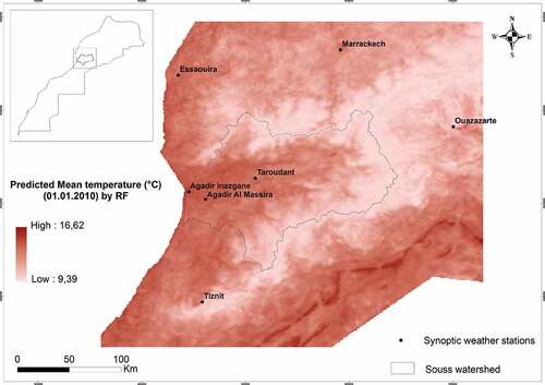
The study area represents the Souss watershed bounded on the north, south, east, and west by the High Atlas Mountains, the Anti-Atlas Mountains, the Siroua Massif and the Atlantic Ocean, respectively, in southwest Morocco (Figure 1). Elevation is variable in the region, ranging from sea level to 4122 m at the highest peak. Due to the scarcity of in situ weather observations in the watershed, the available climate data in the watershed lacks adequate coverage.

Figure 1. Map of the Souss watershed showing the selected weather stations.

2.2. Data

2.2.1. Satellite and remote sensing data

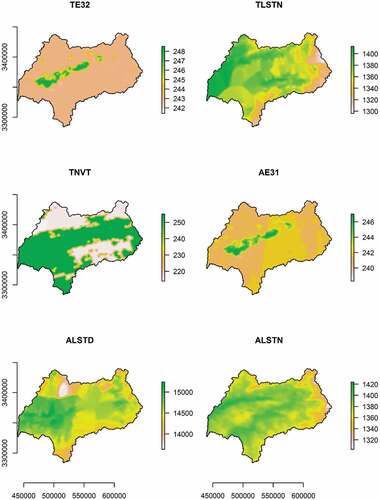
MODIS Terra and Aqua daily LST data were acquired and processed from USGS website using MODIStsp package (Busetto and Ranghetti 2016). MOD11A1 and MYD11A1 are the standard daily LST products derived from the observations of MODIS on board the Terra and Aqua satellites, respectively, and they were used in this study. The MODIS LST data were produced using a generalized split-window algorithm (Wan and Dozier 1996; Li et al. 2013). Filling the gaps in LST products is essential to reduce errors due to problems such as cloud contamination. Several methods, including the improved hybrid approach of Yao et al. (2021) in their study in China. In this study, the fifth order moving average was calculated to fill in the gaps in the MYD11A1 and MOD11A1 data. This calculation was based on the values for the previous 2 days and the next 2 days for a given day, in addition to the values for the days in question. The selected MODIS predictor variables in this study are shown in Figure 2. For the DEM data, it was retrieved from ASTER GDEM website.

Figure 2. MODIS predictor variables for 01/01/2019: Terra Band 32 Emissivity (TE32, unitless, with a 0.002 scale factor), Terra Nighttime Land Surface Temperature (TLSTN, in kelvin with a scale factor of 0.02), Terra local time of night observation (TNVT, in hours with a scale factor of 0.1), Aqua Band 31 Emissivity (AE31, unitless, with a scale factor of 0.002), Aqua Daytime Land Surface Temperature (ALSTD, in kelvin with a scale factor of 0.02) and Aqua Nighttime Land Surface Temperature (ALSTN, in kelvin with a scale factor of 0.02).

2.2.2. Meteorological data

Meteorological data was acquired from the Global Historical Climatology Network-Daily website. Indeed, daily air temperature obtained for seven weather stations, three in and four near the study area (Figure 1) for the period between 2010 and 2019. Due to the existence of several missing data for some stations during the considered period of time, only four synoptic stations were used in the modeling.

2.2.3. Auxiliary data

Air temperature is a consequence of solar radiation, and the spatial and temporal distribution of energy in an area (Barry and Chorley 1987). It is therefore affected by topographic parameters such as elevation, slope, hillshade, and sky-view (Figure 3), which were the four factors were selected as auxiliary predictors in this study.

Figure 3. Auxiliary predictor variables used in the study (elevation in meters, slope in degrees).

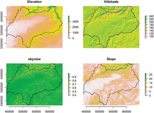
Air temperature decreases with increasing altitude in the troposphere. It is characterized by a decrease in temperature with altitude along the same column of air above the surface. On the other hand, LST exhibits a significant correlation with hillshade, with shaded areas typically having less accumulated solar radiation energy and thus lower temperatures compared to unshaded areas (Peng, Wu, and Zheng 2020). Sky-view measures the portion of the sky visible above the surface from a certain point. It is strongly correlated with diffuse solar radiation, with areas with a high sky-view receiving more solar radiation from the sky than less exposed areas (Robinson 2006). Sky-view is particularly relevant in studies related to heat transfer since the surface generally warms or cools more rapidly when a high portion of the sky is visible (Kokalj, Zaksek, and Ostir 2011). Slope affects the amount of solar radiation received by the surface. Indeed, increasing slope typically causes a gradual downward trend in LST as varying slopes affect the angle of incidence and the reflectivity of solar radiation.

2.2.4. Model training and testing data

The input variables used for training and testing the models included data from MODIS and auxiliary data. In addition, Tair was defined as the response variable for the ML models. The dataset was divided by random partitioning, with 70% and 30% used for the training and validation sets, respectively.

2.3. Modeling

2.3.1. Methods and algorithms used

In this study, two statistical approaches and four ML algorithms were adopted for modeling and the subsequent prediction of Tair. They are presented in Table 1.

Table 1. Statistical and Machine learning methods used for Tair prediction

Method	Description
Linear Regression	Linear regression is a statistical approach that is used to find a linear relationship between the target and one or more predictors. From the target variable (Y), the model aims at making a prediction thanks to the predictor variable (X). Y is usually quantitative, while X can be quantitative or qualitative. The objective is to find a prediction function or a cost function that describes the relationship between X and Y.
Partial Least Squares (PLS)	Based on integration and development of multiple linear regression, canonical correlation analysis, and principal component analysis. Strength lies on its ability to analyze data with strongly collinear, noisy, and numerous (Eriksson et al. 2001).
K-Nearest Neighbors (KNN)	Nonparametric, lazy learning algorithm suitable when there is little or no prior knowledge of the data distribution. Instance-based learning approach where a class label is assigned to a new instance based on the closest correctly classified neighboring instances. Hamming and Euclidean distances are used for discrete and continuous variables, respectively. KNN is based on distance for classification. Thus, if the features represent different physical units or occur at very different scales, normalizing the training data can greatly improve its accuracy. Moreover, it takes all cases contributing to the dataset and ranks the new cases based on their similarity indices. Cases are ranked by voting for neighboring classes, with the optimal case having the highest similarity indices (Wu et al. 2008).
Cubist	Rule-based regression technique that was developed based on a combination of the ideas of Quinlan (1992, 1993). Popular and widely used regression and classification method because due to being ported into R. Has been used in Tair estimation research and showed very good results. Meyer et al. (2016) in mapping daily Tair in Antarctica and Zhang et al. (2006) in estimating daily Tair over the Tibetan plateau in China.
Extreme Gradient Boost (XGB)	Based on aggregation of decision trees. During each iteration, new tree is trained based on the error of the preceding tree Can be used for both classification and regression problems High execution speed out of core computation (Chen and Guestrin 2016) While characterized by generally accurate estimates, the gradient boosting approach can be prone to overfitting. XGB overcomes this limitation by adding a regularization term in the objective function.
Random Forest (RF)	RF, which were proposed by Breiman (2001). Nonparametric, tree-based ensemble technique; Easy to interpret Independent decision trees; developed from bagged set of trees (tree-bagging) In the case of bagging, a number of decision trees are created, each tree being created from a different bootstrap sample of the training dataset. This bootstrap sample refers to a sample of the training dataset where an example may appear more than once in the sample. This is called ”sampling with replacement”. RF operates on multiple decision trees randomly trained on different subsets Final predicted values are produced by the aggregation of the results of all the individual trees that make up the forest (Xu, Knudby, and Ho 2014)

2.3.2. Model training and validation, feature selection, and performance analysis

It is generally preferable to work with a small number of predictors, as this reduces the problem of overfitting, which occurs when the prediction model performs well on the training data but poorly on the test data (Meyer et al. 2016). Indeed, this would avoid the pitfall of failing to predict the Tair of unknown locations despite models accurately predicting Tair for the weather stations used in the training. The leave-one-out cross-validation (LCV) method was used in this study. This approach is appropriate when the data set is small or when an accurate estimate of the model performance is more important than the computational cost of the method. For this study, the period considered for the MODIS and Tair data covers the period between 2010 and 2019. Data splitting was done randomly by taking 70% of the dataset to train the model and the remaining 30% for validation. This was achieved by considering all years rather than selecting separate years to train the model and others to validate it. Feature selection involves reducing the number of input variables when developing a predictive model. In this study, forward feature selection, coupled with LCV, was used to select input variables for modeling. To evaluate the performance of the models, the root mean square error (RMSE) and coefficient of determination (R²) were used. In this study, feature selection was based on spatiotemporal cross-validation using the CreateSpacetimeFolds function in the CAST package (Meyer et al. 2020). The 5-fold approach was used for cross-validation. Models with two predictors are first trained using all possible pairs of predictor variables, with the best model of these initial models retained. Based on this best model, the predictor variables are iteratively increased and each of the remaining variables is tested for its improvement on the current best model. The process stops if none of the remaining variables increases the performance of the model when added to the current best model (Meyer et al. 2020). The Caret package (Kuhn 2014) for R was used for ML model implementations in R.

3. Results

3.1. Feature selection and variable importance

Table 2 shows the selected variables for PLS, RF, and XGB through forward feature selection. Of the 24 considered variables, 11 were selected as relevant in the modeling for PLS, 6 for RF and 9 for XGB. The selected variables for RF were used to train the Cubist and Linear model 1 (LM1), the selected variables for XGB were used to train the XGBD and KNN models and the selected variables for PLS were used to train the Linear model 2 (LM2).

Table 2. Selected variables for PLS, RF, and XGB using forward feature selection

All variables	Models	Selected variables
ACDC (Aqua day clear-sky coverage), ACNC (Aqua night clear-sky coverage), ADVA (Aqua day view angle), ADVT (Aqua day view time), AE31 (Aqua Band 31 Emissivity),AE32 Aqua Band 32 Emissivity, ALSTD (Aqua day land surface temperature), ALSTN (Aqua night land surface temperature), ANVA (Aqua night view angle), ANVT (Aqua night view time),TCDC (Terra day clear-sky coverage),TCNC (Terra night clear-sky coverage), TDVA (Terra day view angle), TDVT (Terra day view time),TE31 (Terra Band 31 Emissivity), TE32 (Terra Band 32 Emissivity),TLSTD (Terra day land surface temperature), TLSTN (Terra night land surface temperature), TNVA (Terra night view angle), TNVT(Terra night view time), Elevation (DEM), Hillshade (HSD), Sky-view, Slope	PLS	ALSTN, TLSTN, HSD, ADVT, ALSTD, ANVA, TLSTD, TCNC, ADVA, TNVA, TNVT
	RF	TE32, TLSTN, ALSTN, ALSTD, TNVT, AE31
	XGB	TE32, TLSTN, ALSTN, AE32, ADVT, DEM, TCNC, TDVT, TLSTD

Figure 4 shows the importance of variables in the modeling. Variables of low relative importance were selected because they increase the accuracy of the model. The feature selection process stops if none of the remaining variables increases model performance when added to the current best model. Only variables that increase model performance were selected, even if they have low relative importance. The importance of a variable refers to the extent to which a given model “uses” that variable to make accurate predictions. The more a model relies on a variable to make predictions, the more important it is to the model. Higher percentages indicate greater importance of the variables. The MODIS TLSTN variable was the most important, scoring 100% in all algorithms except LM2 (93.74%). The MODIS ALSTN variable was highlighted as equally important, scoring second best in all models except Cubist. In addition, the TLSTD and ALSTD variables were found to be important for all models. The high importance of LST in the prediction of Tair as seen in these findings can be explained by the strong correlation between LST and Tair, despite these two differing in physical implications and responses to atmospheric conditions.

Figure 4. Relative variable importance for the algorithms used.

Figure 5 presents the results of the comparison of the methods based on two different validation strategies and two different models: one using all the features and the other using only the features selected after forward feature selection. The aim is to highlight the overfitting problem by showing the differences between the measured and predicted Tair. Indeed, random selection with all features (RS-ALL) and Leave-One -Out Cross-Validation with all features (LCV-ALL) show agreement of models using all predictor variables, while random selection with feature selection (RS-FS) and Leave-One-Out Cross-Validation with feature selection (LCV-FS) show agreement of models using only selected variables. Validation was done either by using random subset representing 70% of total dataset or by LCV

Figure 5. Agreement between measured air temperature and predicted air temperature using RF model as modeling tool. Models were first trained using the full set of predictor variables (ALL) and second using only selected variables as predictors that were revealed during forward feature selection (FS). Two different validation strategies were used: Comparison to a 70% random subset of the total dataset (RS), as well as Leave-One -Out Cross-Validation (LCV).

.

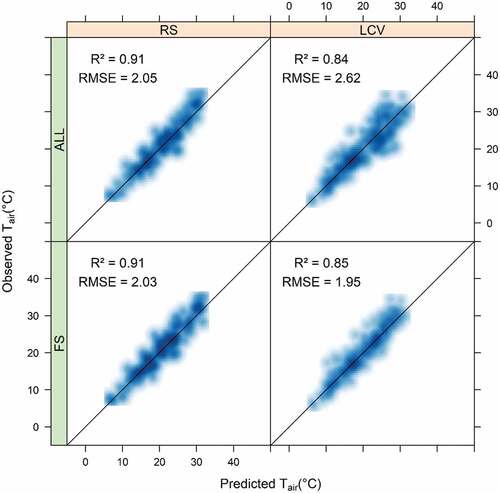
Relatively small errors were observed for all models, with RMSE ranging from 1.95°C to 2.62°C. The smallest errors were observed for the models using feature selection. LCV-FS showed the best fit with R² of 0.85 and RMSE of 1.95°C, while LCV-ALL showed the worst fit, with RMSE of 2.62°C and R² of 0.84.

3.2. Model Comparison and Evaluation

Figure 6 shows the average performance (RMSE, R²) of individual models, which serves as a tool to internally validating models. Overall, the statistical and ML approaches were found to be sufficiently accurate, with RMSE values less than 3°C. This was supported by high R² values, ranging from 0.83 to 0.91, indicating an overall good fit for all models.

Figure 6. Correlation between measured and predicted air temperature based on KNN, PLS, XGB, XGBD, LM1, LM2, CUBIST, and RF models.

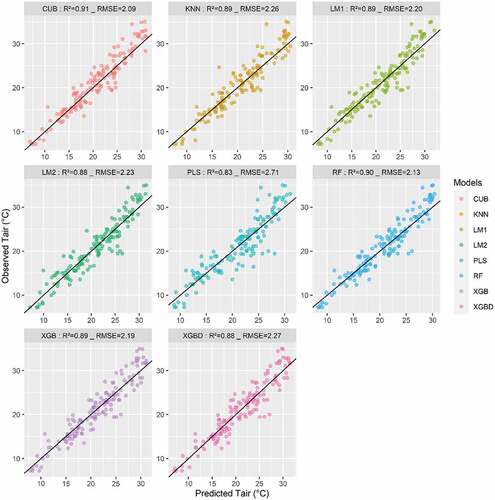
Specifically, Cubist exhibited the highest accuracy, with an RMSE of 2.09°C (R² = 0.91), whereas the least accurate model was the PLS model with an RMSE of 2.71°C (R² = 0.83). It should be noted that the statistical methods (LM1, LM2, and PLS) performed reasonably well, with little difference from the ML models. Nevertheless, the ML approaches generally exhibited the greatest accuracy, with the three best performing models for predicting Tair being Cubist, RF, and XGB with RMSE values of 2.09°C (R² = 0.91), 2.13°C (R² = 0.90), and 2.19°C (R² = 0.89).

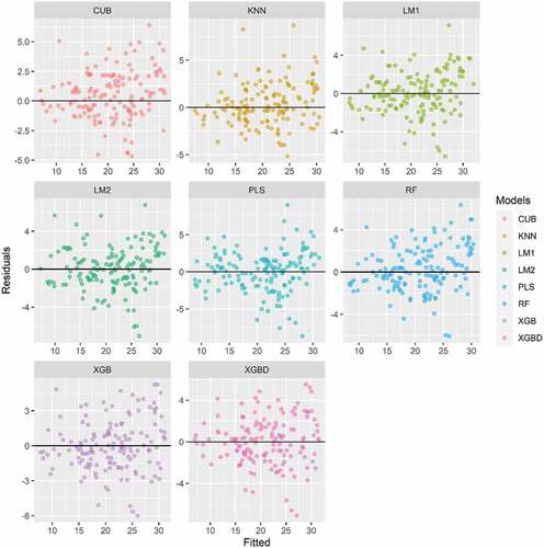
Figure 7 shows the relationship between residuals and fitted values. There is no apparent relationship between residuals and fitted values, this indicates that all models performed quite well.

Figure 7. Distribution of residuals versus fitted air temperature based on KNN, PLS, XGB, XGBD, LM1, LM2, CUBIST, and RF models.

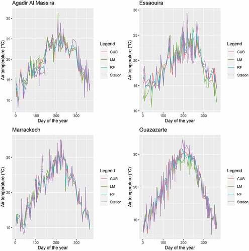
Figure 8 shows a comparison between measured and predicted Tair using cubist, RF, and LM1 for four selected weather stations, namely Agadir Al Massira, Essaouira, Marrakech, and Ouarzazate. Overall, no obvious edge in terms of predictive power is observed for the three models over the four stations. Nevertheless, LM seemed to have difficulties in predicting Tair compared to the other models during the winter months for the Essaouira station. Similarly, its accuracy appeared to be affected in the middle of the year, at the height of summer for the Ouarzazate station, highlighting its potential weakness in predicting the very low and very high Tair corresponding to the winter and summer periods, respectively.

Figure 8. Time series for weather stations: Agadir Al Massira, Essaouira, Marrakech, and Ouarzazate weather stations for 2010–2019 period.

3.3. Station dependent errors

The station-specific error results are presented in Figure 9. The models showed the best performance for Tair prediction for the Marrakech station, with the lowest RMSE at 1.60°C. The highest RMSE was observed for the Essaouira station at 11.46°C for LM1. LM1 appears to have difficulty predicting winter temperatures, as shown in Figure 8 and the high RMSE values in Figure 9.

Figure 9. Station dependent errors: (a) RMSE for RF model, (b) Rsq for RF model, (c) RMSE for CUBIST model, (d) Rsq for CUBIST model, (e) RMSE for KNN model, (f) Rsq for KNN model, (g) RMSE for LM1, (h) Rsq for LM1, (i) RMSE for LM2, (j) Rsq for LM2, (k) RMSE for PLS model, (l) Rsq for PLS model, (m) RMSE for XGB model, (n) Rsq for XGB model, (o) RMSE for XGBD model, (p) Rsq for XGBD model. (For the stations: 1 = Agadir Al Massira, 2 = Essaouira, 3 = Marrackech and 4 = Ouarzazate.).

3.4. Final predicted temperature for the Souss watershed

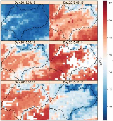
Figures 10–13 present final products, representing the spatiotemporal Tair predictions for daily and monthly aggregates using RF across the Souss watershed. RF was selected because it resulted in the lowest station-dependent errors when taking into account station-dependent error, R², and RMSE. Temperatures are low in winter; gradually increase in spring until reaching the highest values in summer, before starting to decrease in autumn. The monthly evolution of temperatures reveals that the watershed is characterized by a typically Mediterranean climate.

Figure 10. Monthly aggregates of air temperature for 2010 as predicted by the RF model.

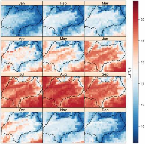
Figure 11. Daily air temperature for 2010 as predicted by the RF model.

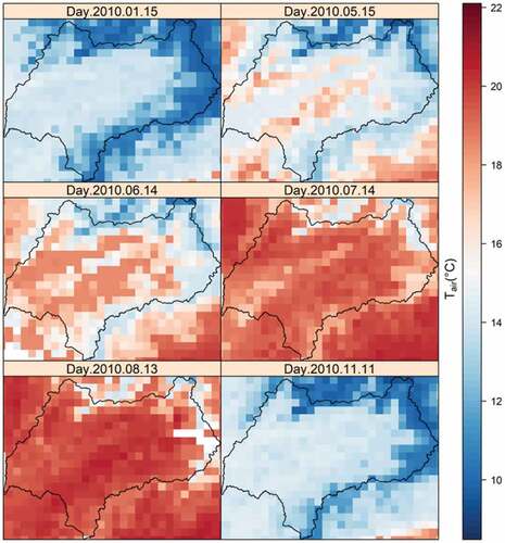
Figure 12. Monthly aggregates of air temperature for 2015 as predicted by the RF model.

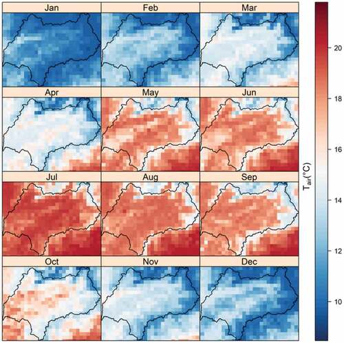
Figure 13. Daily air temperature for 2015 as predicted by the RF model.

4. Discussion

Climate change in Morocco, and more specifically in the Souss region, could be particularly critical for a region whose economy is largely based on subsistence agriculture. This underscores the need for tools capable of monitoring local climate change, including temperature, as management strategies can be adopted based on this.

In this study, MODIS data and weather station data were assembled to estimate Tair for the Souss watershed using ML approaches. Indeed, two statistical models including linear regression and PLS, and four ML algorithms including KNN, Cubist, XGB, and RF were adopted for this purpose. The associated models were generally successful, with RMSE values between 2.09°C and 2.71°C corresponding to the Cubist and the PLS models, respectively. RF model was used to produce maps on Tair estimates over the study area comprising daily and monthly aggregates.

For all models, the average residual was not 0, this implies that the models were systematically biased. The residual analysis revealed that Cubist and KNN had the highest average residuals, with values of 0.52 and 0.36, respectively, while XGB and PLS had the lowest average residuals with values of 0.02 and 0.05, respectively. Thus, although the R² and RMSE values indicate that Cubist performed better than PLS and XGB, the residual analysis revealed that the latter were of a better quality than the former.

Potential issues affecting model performance include insufficient ground data, due to both the limited number of stations and the availability of quality data. Indeed, meteorological data in the Souss watershed were obtained from only seven stations, three of which are characterized by missing data. This scarcity and scattering of weather stations may lead to errors in the modeling compared to areas with sufficient stations. That appeared to be the case in the Meyer et al. (2016) study in Antarctica, where station remoteness likely influenced the prediction of Tair.

5. Conclusions

This study is based on daily and monthly air temperature estimation over the Souss watershed in Morocco using MODIS data and air temperature observations measured at meteorological stations from 2010 to 2019 using six ML algorithms. It highlights the strength of ML tools and remote sensing data in temperature estimation, which has been demonstrated by successful models. LST for the Aqua and Terra sensors was the most relevant predictor in the modeling. ML algorithms such as Cubist and RF were successful in predicting air temperature in the Souss watershed of Morocco, although the differences observed with the often-used linear model were rather small. Future research should focus on how to minimize prediction errors.

Disclosure statement

No potential conflict of interest was reported by the author(s).

Data availability statement

The data that support the findings of this study are openly available at https://earthexplorer.usgs.gov/

Additional information

Notes on contributors

Modeste Meliho

Modeste Meliho is a forest engineer. He received the PhD degree in natural hazards from the Faculty of Science of Rabat. His research interests are ecology and natural resource management, forest sciences, GIS and remote sensing, spatiotemporal modeling, climate change, natural hazards, artificial intelligence, etc.

Abdellatif Khattabi

Abdellatif Khattabi is a professor at the National School of Forestry Engineering (ENFI) of Salé. He is interested in forestry economics, water resources, etc.

Driss Zejli

Driss Zejli is a professor at the National School of Applied Sciences (ENSA) of Kenitra. His research interests are related to renewable energy.

Collins Ashianga Orlando

Collins Ashianga Orlando is a forest engineer. He graduated from the National School of Forestry Engineering (ENFI) of Salé - Morocco.

Caleb E. Dansou

Caleb E. Dansou is a data science student at the School of Information Science (ESI), Rabat, Morocco.

References

- Al Samouly, A., C.N. Luong, Z. Li, S. Smith, B. Baetz, and M. Ghaith. 2018. “Performance of Multi-model Ensembles for the Simulation of Temperature Variability over Ontario, Canada.” Environmental Earth Sciences 77 (13): 1–12. doi:10.1007/s12665-018-7701-2.
- Anderson, M.C., J.M. Norman, W.P. Kustas, R. Houborg, P.J. Starks, and N. Agam. 2008. “A Thermal-based Remote Sensing Technique for Routine Mapping of Land-surface Carbon, Water and Energy Fluxes from Field to Regional Scales.” Remote Sensing of Environment 112: 4227–4241. doi:10.1016/j.rse.2008.07.009.
- Barry, R., and R. Chorley. 1987. Atmosphere, Weather and Climate, 536. 1st ed. Abingdon, UK: Taylor & Francis.
- Breiman, L. 2001. “Random Forests.” Machine Learning 45: 5–32. doi:10.1023/A:1010933404324.
- Busetto, L., and L. Ranghetti. 2016. “MODIStsp: An R Package for Preprocessing of MODIS Land Products Time Series.” Computers & Geosciences 97: 40–48. doi:10.1016/j.cageo.2016.08.020.
- Chen, T., and C. Guestrin. 2016. “XGBoost: A Scalable Tree Boosting System. Association for Computing Machinery.” Paper presented in Proceedings of the 22nd ACM SIGKDD International Conference on Knowledge Discovery and Data Mining. San Francisco, August 13–17. p. 785–794. doi:10.1145/2939672.2939785.
- Dousset, B., and F. Gourmelon. 2003. “Satellite Multi-sensor Data Analysis of Urban Surface Temperatures and Land Cover.” ISPRS Journal of Photogrammetry and Remote Sensing 58 (1–2): 43–54. doi:10.1016/S0924-2716(03)00016-9.
- Eriksson, L., E. Johansson, N. Kettaneh-Wold, and S. Wold. 2001. Multi- and Megavariate Data Analysis: Principles and Applications. Sweden: Umetrics AB.
- Huang, R., C. Zhang, J. Huang, D. Zhu, L. Wang, and J. Liu. 2015. “Mapping of Daily Mean Air Temperature in Agricultural Regions Using Daytime and Nighttime Land Surface Temperatures Derived from TERRA and AQUA MODIS Data.” Remote Sensing 7 (7): 8728–8756. doi:10.3390/rs70708728.
- Karnieli, A., N. Agam, R.T. Pinker, M. Anderson, M.L. Imhoff, and G.G. Gutman. 2010. “Use of NDVI and Land Surface Temperature for Drought Assessment: Merits and Limitations.” Journal of Climate 23: 618–633. doi:10.1175/2009JCLI2900.1.
- Kogan, F.N. 2001. “Operational Space Technology for Global Vegetation Assessment.” Bulletin of the American Meteorological Society 82: 1949–1964. doi:10.1175/1520-0477(2001)082<1949:OSTFGV>2.3.CO;2.
- Kokalj, Z., K. Zaksek, and K. Ostir. 2011. “Application of Sky-view Factor for the Visualisation of Historic Landscape Features in Lidar-derived Relief Models.” Antiquity 85: 263–273. doi:10.1017/S0003598X00067594.
- Kuhn, M. 2014. “Caret: Classification and Regression Training, R Package Version 6.0-29”. CRAN. Wien, Austria, 37.
- Kustas, W., and M. Anderson. 2009. “Advances in Thermal Infrared Remote Sensing for Land Surface Modeling.” Agricultural and Forest Meteorology 149: 2071–2081. doi:10.1016/j.agrformet.2009.05.016.
- Li, X.Y., Z. Li, Q. Zhang, P. Zhou, and W. Huang. 2019. “Prediction of Long-term Near-surface Temperature Based on NA-CORDEX Output.” Journal of Environmental Informatics Letters 2 (4): 10–18.
- Li, Z.L., B.H. Tang, H. Wu, H. Ren, G. Yan, Z. Wan, I. Trigo, and J. Sobrino. 2013. “Satellite-derived land surface temperature: Current status and perspectives.” Remote Sensing of Environment 131 (15): 14–37.
- McMillin, L.M. 1975. “Estimation of Sea Surface Temperature from Two Infrared Window Measurements with Different Absorptions.” Journal of Geophysical Research 80: 5113–5117. doi:10.1029/JC080i036p05113.
- Meyer, H., C. Reudenbach, M. Ludwig, T. Nauss, and E. Pebesma. 2020. “Package ‘CAST’.” CRAN. Wien, Austria, 13.
- Meyer, H., M. Katurji, T. Appelhans, M.U. Müller, T. Nauss, P. Roudier, and P. Zawar-Reza. 2016. “Mapping Daily Air Temperature for Antarctica Based on MODIS LST.” Remote Sensing 8: 732. doi:10.3390/rs8090732.
- Modeste Meliho. 2019. “Soil Erosion Risk Assessment in Relationship to Land Uses and Vegetation Cover through Rainfall Simulations, 137Cs Radioactive Tracer and Modelisation based on GIS and Remote Sensing (High Atlas, Morocco).” PhD diss., Université Mohammed V – Faculté des Sciences de Rabat, 1-168.
- Peng, X., W. Wu, and Y. Zheng. 2020. “Correlation Analysis of Land Surface Temperature and Topographic Elements in Hangzhou, China.” Scientific Reports 10: 10451. doi:10.1038/s41598-020-67423-6.
- Quinlan, J.R., 1992. “Learning with Continuous Classes.” In Proceedings of the 5th Australian Joint Conference on Artificial Intelligence, 343–348. Hobart, Tasmania, November 16–18.
- Quinlan, J.R., 1993. “Combining Instance-based and Model-based Learning”. In Proceedings of the Tenth International Conference on Machine Learning, 236–243. Amherst, MA, USA, June 27–29.
- Robinson, D. 2006. “Urban Morphology and Indicators of Radiation Availability.” Solar Energy 80: 1643–1648. doi:10.1016/j.solener.2006.01.007.
- Serra, C., X. Lana, M.D. Martınez, J. Roca, B. Arellano, R. Biere, M. Moix, and A. Burgueno. 2020. “Air Temperature in Barcelona Metropolitan Region from MODIS Satellite and GIS Data.” Theoretical and Applied Climatology 139 (1–2): 473–492. doi:10.1007/s00704-019-02973-y.
- Shah, D.B., M.R. Pandya, H.J. Trivedi, and A.R. Jani. 2012. “Estimation of Minimum and Maximum Air Temperature Using MODIS Data over Gujarat.” Journal of Agrometeorology 14 (2): 111–118.
- Su, Z. 2002. “The Surface Energy Balance System (SEBS) for Estimation of Turbulent Heat Fluxes.” Hydrology and Earth System Sciences 6: 85–100. doi:10.5194/hess-6-85-2002.
- Wan, Z., and Dozier, J. 1996. “A generalized split-window algorithm for retrieving landsurface temperature from space.” IEEE Transactions on Geoscience and Remote Sensing 34: 892–905.
- Wu, X., V. Kumar, J.R. Quinlan, J. Ghosh, Q. Yang, H. Motoda, G.J. McLachlan, A. Ng, B. Liu, and S.Y. Philip. 2008. “Top 10 Algorithms in Data Mining.” Knowledge and Information Systems 14: 1–37. doi:10.1007/s10115-007-0114-2.
- Xu, Y., A. Knudby, and H.C. Ho. 2014. “Estimating Daily Maximum Air Temperature from MODIS in British Columbia, Canada.” International Journal of Remote Sensing 35: 8108–8121. doi:10.1080/01431161.2014.978957.
- Yao, R., L. Wang, X. Huang, L. Li, J. Sun, X. Wu, and W. Jiang. 2020. “Developing a Temporally Accurate Air Temperature Dataset for Mainland China.” Science of the Total Environment 706: 136037. doi:10.1016/j.scitotenv.2019.136037.
- Yao, R., X. Huang, L. Sun, R. Chen, X. Wu, W. Zhang, and Z. Niu. 2021. “A Robust Method for Filling the Gaps in MODIS and VIIRS Land Surface Temperature Data.” IEEE Transactions on Geoscience and Remote Sensing. (online published). doi:10.1109/TGRS.2021.3053284.
- Zhang, H., F. Zhang, M. Ye, T. Che, and G. Zhang. 2006. “Estimating Daily Air Temperatures over the Tibetan Plateau by Dynamically Integrating MODIS LST Data.” Journal of Geophysical Research: Atmospheres 121: 11425–11441.
- Zhang, R., J. Tian, H. Su, X. Sun, S. Chen, and J. Xia. 2008. “Two Improvements of an Operational Two-layer Model for Terrestrial Surface Heat Flux Retrieval.” Sensors 8: 6165–6187. doi:10.3390/s8106165.