Land cover classification from remote sensing images based on multi-scale fully convolutional network

ABSTRACT

Although the Convolutional Neural Network (CNN) has shown great potential for land cover classification, the frequently used single-scale convolution kernel limits the scope of information extraction. Therefore, we propose a Multi-Scale Fully Convolutional Network (MSFCN) with a multi-scale convolutional kernel as well as a Channel Attention Block (CAB) and a Global Pooling Module (GPM) in this paper to exploit discriminative representations from two-dimensional (2D) satellite images. Meanwhile, to explore the ability of the proposed MSFCN for spatio-temporal images, we expand our MSFCN to three-dimension using three-dimensional (3D) CNN, capable of harnessing each land cover category’s time series interaction from the reshaped spatio-temporal remote sensing images. To verify the effectiveness of the proposed MSFCN, we conduct experiments on two spatial datasets and two spatio-temporal datasets. The proposed MSFCN achieves 60.366% on the WHDLD dataset and 75.127% on the GID dataset in terms of mIoU index while the figures for two spatio-temporal datasets are 87.753% and 77.156%. Extensive comparative experiments and ablation studies demonstrate the effectiveness of the proposed MSFCN. Code will be available at https://github.com/lironui/MSFCN.

KEYWORDS:

• Spatio-temporal remote sensing images
• Multi-Scale Fully Convolutional Network
• land cover classification

1. Introduction

Land cover classification is a foundational technology for land resource management, cultivated area evaluation, and economic assessment, which is significant for homeland security and national economic stability (Li et al. 2021a; Zhang, Feng, and Yao 2014; Ramli and Tahar 2020; Qi et al. 2020). Conventionally, large-scale field surveys are the primary method to obtain land use and land cover. Although the outcomes of surveys are normally of high quality, the investigative procedures are time-consuming and labor-intensive. Meanwhile, the information about the geographical distribution of land cover is often missing (Basso and Liu 2019; Zhang et al. 2019a).

As a powerful Earth observation technology, remote sensing can capture Earth’s surface images via sensors on aircraft or satellites without physical contact (Duan, Pan, and Li 2020; Zhong et al. 2018; Wang et al. 2021b). Optical remote sensing is a significant branch of remote sensing and has been applied in many fields, including super-resolution land cover mapping (Wang et al. 2019b), drinking water protection (Wang et al. 2019a), and object detection (Zhang et al. 2019b). Scholars have increasingly focused on automatic land cover classification using satellite images by profiting from the substantial remote sensing images (Prins and Van Niekerk 2020; Shao, Wu, and Li 2021; Li et al. 2021e).

Generally, remote sensing classification models consist of two procedures, namely feature engineering and classifier training. The former aims to transform spatial, spectral, or temporal information into discriminative feature vectors. The latter is designed to train a general-purpose classifier to classify the feature vectors into the correct category. When it comes to land cover classification, vegetation indices are one genre of frequently used features extracted from multi-spectral/multi-temporal images to manifest the physical properties of land cover. The Normalized Difference Vegetation Index (NDVI) (Tucker 1979) and Soil-Adjusted Vegetation Index (SAVI) (Huete 1988) highlight vegetation. The Normalized Difference Bareness Index (NDBaI) (Zhao and Chen 2005) and the Normalized Difference bare Land Index (NBLI) (Li et al. 2017) emphasize bare land. The Normalized Difference Water Index (NDWI) (Gao 1996) and Modified NDWI (MNDWI) (Xu 2006) indicate water. Besides, the object-based approach utilizing geographic objects as basic units for land cover classification is another thriving area that generally reduces the within-class variation and removes salt-and-pepper effects (Georganos et al. 2018; Matikainen et al. 2017).

Meanwhile, the remote sensing community has tried to design various classifiers from diverse perspectives (Wu, Gui, and Yang 2020; Dela Torre, Gao, and Macinnis-Ng 2021; Yang et al. 2020), from orthodox methods such as logistic regression (Rutherford, Guisan, and Zimmermann 2007), distance measure (Du and Chein 2001), and clustering (Maulik and Saha 2010), to advanced techniques including Support Vector Machine (SVM) (Zafari, Zurita-Milla, and Izquierdo-Verdiguier 2020), Random Forest (RF) (Tatsumi et al. 2015), and Multi-Layer Perceptron (MLP) (Zhang et al. 2018). Since extraction of the geographical distribution of land cover requires pixel-based image classification, precisely refined pixel features are pivotal for these classifiers. However, the high dependency on manual descriptors restricts the flexibility and adaptability of these methods.

The emergence of Deep Learning (DL), which is powerful to capture nonlinear and hierarchical features automatically, tackles the above deficiency to a great extent (Li et al. 2021c). DL has influenced many domains, such as Computer Vision (CV), Natural Language Processing (NLP), as well as Automatic Speech Recognition (ASR). As a typical classification task (Zhong et al. 2018; Shao, Wu, and Li 2021), a great many DL methods have been introduced to land cover classification (Wang et al. 2021a). Compared to vegetation indices that only consider finite bands, DL methods can harness various information, including periods, spectrums, and the interactions between different kinds of land cover.

Zhong, Hu, and Zhou (2019) exploited temporal features using a one-dimensional (1D) CNN to recognize the intricate seasonal dynamics of economic crops and lessened the dependency on hand-crafted feature engineering. Pelletier, Webb, and Petitjean (2019) proposed a temporal CNN for satellite image time series. They proved the significance of harnessing the information both in spectral dimension and temporal dimension when implementing the convolutions. Based on fine-tuned CNN, Tong et al. (2020) combined hierarchical segmentation and patch-wise classification for land cover classification. Specifically, many cutting-edge technologies used in semantic segmentation, whose task is assigning each pixel with a specific category (Chen et al. 2020), have also been generalized to land cover classification (Heipke and Rottensteiner 2020). Inspired by the progress in the encoder-decoder Fully Convolutional Network (FCN) framework, Li et al. (2021a) improved the U-Net with asymmetric convolution for fine-resolution remote images. Meanwhile, the attention mechanism has also been introduced for remote sensing images (Li et al. 2021b, 2021d).

Even though the encoder-decoder FCN framework (Badrinarayanan, Kendall, and Cipolla 2017; Chen et al. 2018; Ronneberger, Fischer, and Brox 2015) has been an essential structure for land cover classification (Liu et al. 2020; Mohammadimanesh et al. 2019; Sang et al. 2019), the single-scale convolution kernel limits the scope of information extraction. To remedy this drawback, we propose a Multi-Scale Fully Convolutional Network based on encoder-decoder FCN structure to exploit both local and global features from satellite images. We design two branches with convolutional layers in different kernel sizes in each layer of the encoder to capture multi-scale features. In addition, a channel attention block and a global pooling module (Ji et al. 2020) enhance channel consistency and global contextual consistency.

At the same time, spatio-temporal satellite images, bolstered by their increasing attainability, are at the forefront of a comprehensive effort towards automatic Earth monitoring by international agencies (Sainte Fare Garnot et al. 2020). However, when utilizing the 2D CNN to extract features from spatio-temporal satellite images, the temporal dimensions of the extracted features generated by the convolution layer must be averaged and devastated to a scalar, which collapses the time-series information contained in multi-temporal images. Many studies have been conducted motivated by NLP’s progress to cope with this defect. Rußwurm and Körner (2018) adapted sequence encoders to represent Sentinel 2 images’ temporal sequence and alleviated the demand of humdrum and cumbersome cloud-filtering. Interdonato et al. (2019) designed a two-branch architecture with an RNN branch to extract temporal features and a CNN branch to extract spatial features. By incorporating both CNN and RNN, Rustowicz et al. (2019) designed a 2D U-Net + CLSTM model for spatio-temporal satellite images. Meanwhile, for embedding time-sequences, Transformer architecture was introduced into land cover classification using spatio-temporal satellite images by Sainte Fare Garnot et al. (2020). All these attempts have made encouraging progress and broadened the boundaries of this field.

In the meantime, the advent of 3D CNN solves the dilemma mentioned above from another facet. Unlike traditional 2D CNN which operates on 2D images, 3D CNN implements convolutional operation on three dimensions, which naturally fits feature extraction from data represented in 3D format. Thus, 3D CNN has been utilized for video understanding (Wu et al. 2019), point clouds representation (Hamraz et al. 2019), 3D object detection based on Light Detection and Ranging (LiDAR) data (Gong et al. 2020), hyperspectral images classification (Li et al. 2020), and multi-temporal images segmentation (Ji et al. 2018). As remote sensing images normally comprise much temporal, dynamic, or spectral information, like the whole crop growth cycle in the temporal dimension, 3D CNN is a superexcellent method to extract these features.

Using multi-temporal images, Ji et al. (2018) designed a 3D-CNN-based segmentation model for crop classification. As the temporal dimension is reserved, the model’s performance surpassed the 2D-CNN-based methods and other traditional classifiers. However, as 3D CNN is a computationally intensive operation, the pixel-by-pixel segmented procedure requires numerous computational resources (Ji et al. 2018). Thus, based on the idea of semantic segmentation, Ji et al. (2020) proposed a novel 3D encoder-decoder FCN framework with global pooling and attention mechanism (3D FGC), which was able to capture feature maps from the whole input and improves both the accuracy and the efficiency.

Based on the insight and progress mentioned above, we extend our Multi-Scale Fully Convolutional Network to three-dimension based on 3D CNN for land cover classification using spatio-temporal satellite images. To verify the effectiveness, we compare the performance of 2D MSFCN with SegNet (Badrinarayanan, Kendall, and Cipolla 2017), FC-DenseNet (Jegou et al. 2017), U-Net (Ronneberger, Fischer, and Brox 2015), Attention U-Net (Oktay et al. 2018) and FGC (Ji et al. 2020), and the performance of 3D MSFCN with 1D U-Net, 2D U-Net (Ronneberger, Fischer, and Brox 2015), 3D U-Net (Ronneberger, Fischer, and Brox 2015), 3D Attention U-Net (Oktay et al. 2018), Conv-LSTM (Rußwurm and Körner 2018) and 3D FGC (Ji et al. 2020). The main contributions of this paper could be listed as follows:

• To expand the scope of information extraction in the spatial domain, we designed a Multi-Scale Convolutional Block (MSCB), which can capture the input’s local and global features, respectively.

• Based on MSCB, we proposed a Multi-Scale Fully Convolutional Network (MSFCN) with channel attention block and global pooling module, and extend MSFCN for 3D spatio-temporal satellite images.

• A series of quantitative experiments on two spatial datasets and two spatio-temporal datasets show the effectiveness of the proposed MSFCN.

This paper’s remainder is arranged as follows: In Section 2, taking 3D MSFCN as an example, we illustrate the detailed structure of the proposed framework. The experimental results are provided and analyzed in Section 3. Finally, in Section 4, we conclude the entire paper.

2. Methodology

2.1. Feature extraction using 3D CNN

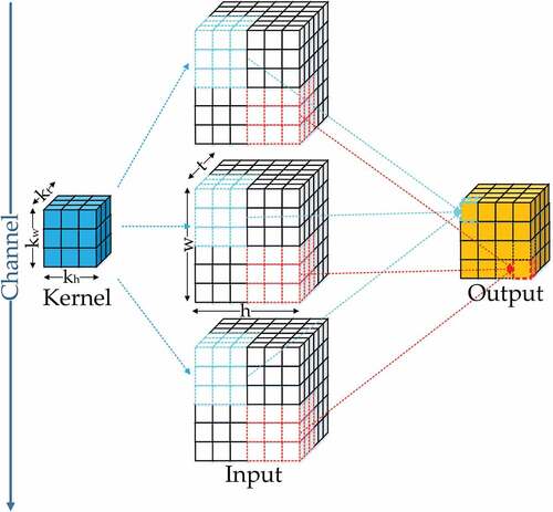
3D CNN is capable of capturing spatial and temporal features simultaneously, and Batch Normalization (BN) layer (Ioffe and Szegedy 2015) is often appended to improve numerical stability. Thus, we consider 3D CNN with a BN layer as an example to elaborate on 3D CNN’s mechanism. Supposing that the size of input 3D feature maps is expressed as $\left(\mathit{t}\times \mathit{h}\times \mathit{w},\mathit{c}\right)$, and the shape of the convolution kernel is $\left(k_t\times k_h\times k_w\right)$, where t, h, w, and c denote the dimension of time series, height, width, and channels. The convolution operations are implemented based on the convolution kernel and sliding windows in the shape of $\left(k_t\times k_h\times k_w\right)$. The obtained values constitute the output 3D feature maps. Another important parameter, stride, determines the distance of width and height traversed per slide of the sliding windows. A diagrammatic sketch with one kernel can be seen in Figure 1. Concretely, the operation of 3D CNN can be formalized as:

(1) ${\mathit{x}}_{i,j}^{t,h,w}=\sum _m\sum _{\mathit{p}=0}^{T_i-1}\sum _{\mathit{q}=0}^{H_i-1}\sum _{\mathit{r}=0}^{W_i-1}\begin{array}{c}{\mathit{W}}_{i,j,m}^{p,q,r}{\mathit{x}}_{i-1,m}^{\left(t+p\right),\left(h+q\right),\left(w+r\right)}+b_{\mathit{i},\mathit{j}}\end{array}$(1)

Figure 1. 3D convolution indicates convolution operator is implemented in three directions (i.e. two spatial directions and a temporal direction) sequentially. Both the input feature maps and the output feature maps are 3D tensors.

where ${\mathit{x}}_{i,j}^{t,h,w}$ denotes the $\mathit{j}$-th feature cube at position $\left(\mathit{t},\mathit{h},\mathit{w}\right)$ in the $\mathit{i}$ th layer. $\mathit{m}$ means the feature maps generated by the $\left(\mathit{i}-1\right)$-th layer. ${\mathit{W}}_{i,j,m}^{p,q,r}$ represents the column weight of the $\mathit{m}$ th feature cube at position $\left(\mathit{p},\mathit{q},\mathit{r}\right)$. $b_{\mathit{i},\mathit{j}}$ is the $\mathit{j}$ th feature cube in the $\mathit{i}$ th layer’s bias items of the filter. $T_i$ means the convolution kernel along the temporal dimension of input spatio-temporal satellite images, while $H_i$ and $W_i$ respectively express the height and width of the kernel in the spatial dimension.

Then, the generated 3D feature maps ${\mathit{x}}_i$ is fed into the BN layer and normalized as:

(2) $\widehat{x_i}=\frac{{\mathit{x}}_i-\mathit{E}\left({\mathit{x}}_i\right)}{\sqrt{\mathit{Var}\left({\mathit{x}}_i\right)+\mathit{ϵ}}}$(2)

(3) ${\mathit{y}}_i=\mathit{\sigma }\left({\gamma }_i{\hat{\mathit{x}}}_{\mathit{i}}+{\beta }_i\right)$(3)

where $y_i$ is the output of the BN layer. $\mathit{Var}\left(\cdot \right)$ and $\mathit{E}\left(\cdot \right)$ represent the variance function and expectation of the input, respectively. ε is a small constant to maintain numerical stability. $\mathit{\gamma }$ and $\mathit{\beta }$ are two trainable parameters, and the normalized result ${\hat{\mathit{x}}}_{\mathit{i}}$ can be scaled by $\mathit{\gamma }$ and shifted by $\mathit{\beta }$. $\mathit{\sigma }\left(\cdot \right)$ denotes the activation function, which is set as ReLU in our model.

As the quality of extracted features limits the performance of the model and the convolution kernel size determines the receptive field, how to design the size of the convolution kernel is the core of the network.

2.2. Multi-Scale Convolutional Block

Generally, the larger convolution kernel size means the larger receptive field and the more global vision, which augments the scope of areas observed in the image. Conversely, the decrease in the convolution kernel size would shrink the receptive field and obtain the local vision. However, both the global visual patterns and the local the visual patterns contain visual features. Thus, a fully convolutional neural network’s evident imperfection is the same size convolutional kernels, leading to a constant receptive field. As shown in Figure 2(a), the conventional convolutional block used in FCN usually contains two stacked 3D CNN with the activation function. To expand the receptive field, in MSFCN, we design a Multi-Scale Convolutional Block (MSCB) to exploit the global and local features simultaneously.

Figure 2. Comparison of (a) conventional convolution block and (b) multi-scale convolution block.

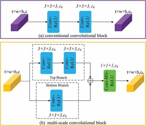
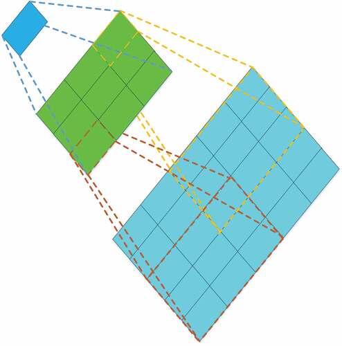
The structure of the multi-scale fully convolutional layer can be seen in Figure 2(b). Similarly, supposing the input 3D feature maps is in the shape of $\left(\mathit{t}\times \mathit{h}\times \mathit{w},\mathit{c}\right)$, where the t, h, w, and c represent the time series, height, width, and channels of the input, respectively. The top branch of the block contains two stacked $\left(3\times 3\times 3\right)$ convolution layers, and the receptive field of two stacked $\left(3\times 3\times 3\right)$ convolution layers are equivalent to a $\left(5\times 5\times 5\right)$ convolution layer. An illustration in 2D format can be seen in Figure 3. Thus, the top branch is capable of capturing more global visual patterns. Meanwhile, the block’s bottom branch harnesses a single $\left(3\times 3\times 3\right)$ convolution layer that exploits local visual patterns.

Figure 3. The receptive field of two stacked (3 × 3) convolution layers is equivalent to a (5 × 5) convolution layer.

Subsequently, the add operation is implemented between the outputs of the top branch and the bottom branch, and obtains the feature maps with the size of $\left(\mathit{t}\times \mathit{h}\times \mathit{w},c_k\right)$. Finally, the extracted feature maps are fed into a $\left(1\times 1\times 1\right)$ convolution layer with the BN layer to further increase the nonlinear characteristics and characterization capabilities of the block.

2.3. Channel attention block and global pooling module

In the FCN framework, the convolution operator’s output is a score map, which indicates the probability of each class at each pixel. And to attain the final score map, all channels of feature maps are simply summed as:

(4) $y_n=\mathit{F}\left(\mathit{x};\mathit{\omega }\right)=\sum _{\mathit{i}=1,\mathit{j}=1,\mathit{k}=1}^D{\omega }_{\mathit{i},\mathit{j},\mathit{k}}{x}_{\mathit{i},\mathit{j},\mathit{k}}$(4)

where $\mathit{\omega }$ denotes the convolution kernel. $\mathit{x}$ represents the feature maps generated by the network. $\mathit{D}$ is the set of pixel positions. And $\mathit{n}\in \left\{1,2,\dots ,\mathit{N}\right\}$, where $\mathit{N}$ indicates the number of channels. Then the prediction probability is calculated as:

(5) ${\delta }_i\left(y_n\right)=\frac{\exp \left(y_n\right)}{{\sum }_{j=1}^K\exp \left(y_j\right)}$(5)

where $\mathit{y}$ denotes the output of the network, and $\mathit{\delta }$ indicates the prediction probability. The category with the highest probability is the final predicted label, deduced by Equations (4(4) $y_n=\mathit{F}\left(\mathit{x};\mathit{\omega }\right)=\sum _{\mathit{i}=1,\mathit{j}=1,\mathit{k}=1}^D{\omega }_{\mathit{i},\mathit{j},\mathit{k}}{x}_{\mathit{i},\mathit{j},\mathit{k}}$(4) ) and (5(5) ${\delta }_i\left(y_n\right)=\frac{\exp \left(y_n\right)}{{\sum }_{j=1}^K\exp \left(y_j\right)}$(5) ). Nevertheless, Equation (4)(4) $y_n=\mathit{F}\left(\mathit{x};\mathit{\omega }\right)=\sum _{\mathit{i}=1,\mathit{j}=1,\mathit{k}=1}^D{\omega }_{\mathit{i},\mathit{j},\mathit{k}}{x}_{\mathit{i},\mathit{j},\mathit{k}}$(4) impliedly demonstrates that all channels share equal weights. However, the features generated by different stages own different levels of discrimination, which causes different consistency in prediction.

Supposing the prediction label is $y_0$ and that the corresponding true label is $y_1$, we can modify the highest probability value from $y_0$ to $y_1$ by introducing a parameter $\mathit{\alpha }$:

(6) $\bar{y}=\mathit{\alpha y}=\left[\begin{array}{c}{\alpha }_1\\ ⋮\\ {\alpha }_N\end{array}\right]\cdot \left[\begin{array}{c}{y}_1\\ ⋮\\ y_N\end{array}\right]=\left[\begin{array}{c}{\alpha }_1{\omega }_1\\ ⋮\\ {\alpha }_N{\omega }_N\end{array}\right]\times \left[\begin{array}{c}{x}_1\\ ⋮\\ x_N\end{array}\right]$(6)

in which $\mathit{\alpha }=\mathit{Sigmoid}\left(\mathit{x};\mathit{w}\right)$ and $\bar{y}$ is the new prediction label of the network. As can be seen from Equation (6)(6) $\bar{y}=\mathit{\alpha y}=\left[\begin{array}{c}{\alpha }_1\\ ⋮\\ {\alpha }_N\end{array}\right]\cdot \left[\begin{array}{c}{y}_1\\ ⋮\\ y_N\end{array}\right]=\left[\begin{array}{c}{\alpha }_1{\omega }_1\\ ⋮\\ {\alpha }_N{\omega }_N\end{array}\right]\times \left[\begin{array}{c}{x}_1\\ ⋮\\ x_N\end{array}\right]$(6) , the value of $\mathit{\alpha }$ refines the feature maps $\mathit{x}$ and enhances the discriminative features as well as restrains the indiscriminative features. The channel attention block is designed based on the insight mentioned above (Yu et al. 2018) and is expanded to the 3D version (Ji et al. 2020).

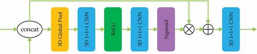
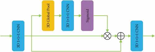
The CAB structure can be seen in Figure 4, whose input is the concatenated feature maps extracted by the encoder and decoder. First, a 3D global average pooling layer in CAB exploits the input’s global context, and sequentially two $\left(1\times 1\times 1\right)$ convolution layers with ReLU and sigmoid activation function adaptively realign the channel-wise dependencies. The weight vector generated by CAB manifests the relative significance between the channel-wise features and enhances the discriminability of features. Subsequently, the multiplication operation and addition operation are operated between the output vector and the input feature maps. Finally, the last $\left(1\times 1\times 1\right)$ convolution layer is designed to generate globally consistent spatio-temporal feature maps. Through re-modeling the channel-wise features, the 3D Channel Attention Block (CAB) fuses the spatio-temporal features between the encoder and the decoder.

Figure 4. The structure of the Channel Attention Block (CAB).

Meanwhile, context is utile information that can enhance segmentation and detection performance using deep learning (Liu, Rabinovich, and Berg 2015). As for land cover classification, local semantic information contained per pixel is often equivocal. By taking contextual information into account, semantic information will be enhanced. Global average pooling is an effective method to capture the global contextual prior (Liu, Rabinovich, and Berg 2015). Based on the idea that a global average pooling layer can improve the spatio-temporal consistency on the highest level of the encoder (the top semantic layer), the Global Pooling Module (GPM) is elaborately designed (Ji et al. 2020), which can be seen in Figure 5. Meanwhile, with global spatio-temporal consistency, the GPM transforms the feature maps at the highest level of the encoder to the decoder’s corresponding feature maps. Like the CAB, GMP’s effect is reweighting feature maps, which can also be seen as an attention mechanism.

Figure 5. The structure of the Global Pooling Module (GPM).

The structure of the GMP can be seen in Figure 5. First, the input feature maps are fed into a $\left(1\times 1\times 1\right)$ convolution layer. Then, a 3D global average pooling and a $\left(1\times 1\times 1\right)$ convolution layer with a sigmoid activation function are attached. Finally, the multiplication operation and addition operation are implemented between the generated vector and the first convolution layer’s output. The final output is processed by the last $\left(1\times 1\times 1\right)$ convolution layer to acquire the decoder’s highest layer.

2.4. Network architecture

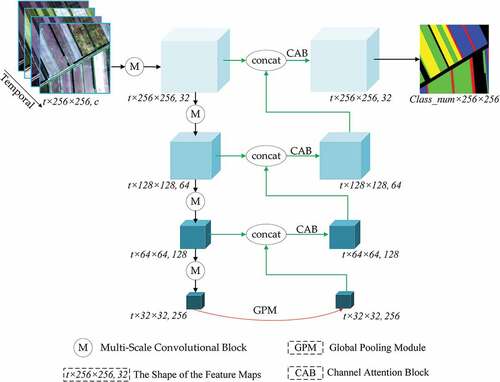
Based on the 3D CNN, the multi-scale convolutional block, the channel attention block, and the global pooling module, we construct the MSFCN for land cover classification from satellite images, as shown in Figure 6. For two spatio-temporal datasets, the input image is in $\mathit{t}\times 256\times 256,\mathit{c}$, where $\mathit{t}=4$ is the number of images along the temporal dimension and $\mathit{c}=4$ is the number of channels. The encoder of the MSFCN comprises four multi-scale convolutional blocks with the output channels as 32, 64, 128, and 256, respectively, and the number of layers and channels will be discussed in Section 3.6. After each multi-scale convolutional block, the max-pooling layer with $\left(1\times 2\times 2\right)$ kernel is applied, which reserves the temporal information and condenses the spatial information. At the highest layer of the encoder, the GPM is utilized to enhance the global spatio-temporal consistency. Then, using CAB, the feature maps from the encoder and decoder are fused, and the output of each layer in the decoder is sequentially restored up to the input size via the transposed convolution layer with $\left(1\times 2\times 2\right)$ kernel. After each transposed convolution layer, a $\left(3\times 3\times 3\right)$ convolution layer is attached to avoid the checkerboard pattern caused by the transposed convolution. In the end, the final 3D feature maps are fed into a $\left(\mathit{t}\times 3\times 3\right)$ convolution layer and a $\left(1\times 1\times 1\right)$ convolution layer to coalesce time dimension and generate 2D segmentation maps.

Figure 6. The structure of the proposed MSFCN network.

Following the pioneering works (Ji et al. 2018, 2020), we adopt the most commonly used cross-entropy loss function as the quantitative evaluation and backpropagation index to measure the disparity between the obtained 2D segmentation maps and ground truth, which is defined as:

(7) $\mathit{los}{s}_{\mathit{i},\mathit{j}}=-\sum _k{q}_{\mathit{i},\mathit{j},\mathit{k}}log{p}_{\mathit{i},\mathit{j},\mathit{k}}$(7)

(8) $\mathit{loss}=\frac{1}{N}\sum _i\sum _j\mathit{los}{s}_{\mathit{i},\mathit{j}}$(8)

where $p_{\mathit{i},\mathit{j}}$ is the predicted category probability distribution of pixel $\left(\mathit{i},\mathit{j}\right)$, $q_{\mathit{i},\mathit{j}}$ is the actual category probability distribution of pixel $\left(\mathit{i},\mathit{j}\right)$, $\mathit{k}$ represents the number of classes, and $\mathit{N}$ denotes the number of pixels.

3. Experimental results

This section first introduces the datasets and experimental settings to verify the effectiveness of MSFCN and then compares the performance between different frameworks.

3.1. Dataset

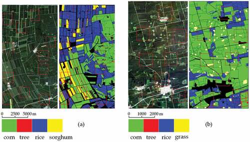
The effectiveness of 2D MSFCN is verified using Wuhan Dense Labeling Dataset (WHDLD) (Shao et al. 2020) and Gaofen Image Dataset (GID), which can be seen in Figures 7 and 8. The effectiveness of 3D MSFCN is verified using two Gaofen 2 (GF2) spatio-temporal satellite images (Tong et al. 2020), which can be seen in Figure 9.

Figure 7. Examples of WHDLD images and their corresponding ground truth.

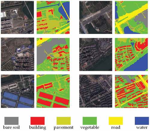
Figure 8. Examples of GID images and their corresponding ground truth.

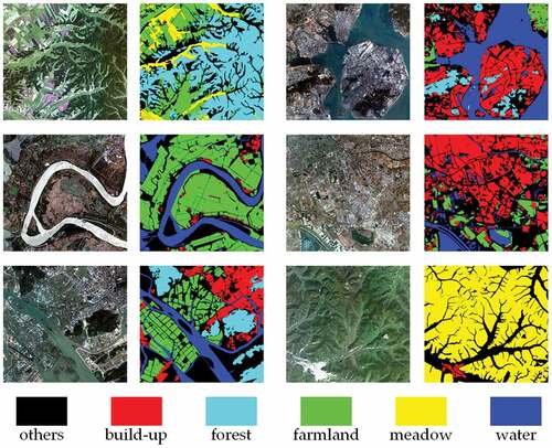
Figure 9. GF2 datasets gathered in (a) 2015, and (b) 2017. Each dataset owns four crop species labeled in different colors, and black pixels represent label information is absent. Patches indicated in red rectangles were utilized to train the network and the remainder to prediction.

WHDLD contains 4940 RGB images in 256 × 256 captured by Gaofen 1 Satellite and ZY-3 Satellite over Wuhan urban area. By image fusion and resampling, the resolution of the images reaches 2 m/pixel. The images contained in WHDLD are labeled with six classes, bare soil, building, pavement, vegetation, road, and water.

GID contains 150 RGB images in 7200 × 6800 captured by Gaofen 2 Satellite over 60 cities in China. Each image covers a geographic region of 506 km². The GID images are labeled with six classes, build-up forest, farmland, meadow, water, and others. However, as we do not have enough computing resources to cope with such extremely enormous pixels, we just select 15 images contained in GID. The principle of selection is to cover the whole six classes. And the serial number of the chosen images will be released with our open-source code.

The two spatio-temporal satellite datasets that own four bands (red, green, blue, and near-infrared) in 4 m ground resolution were gathered in 2015 and 2017, respectively. For the 2015 dataset, there are four images collected in June, July, August, and September in the year 2015, and 2652 × 1417 pixels of each image. The 2017 dataset comprises seven images with 2102 × 1163 pixels captured in June, July, August, September, October, November, and December in 2017. Two GF2 datasets are preprocessed with quick atmospheric correction and geometrical rectification.

3.2. Experimental setting

To evaluate the effectiveness of 2D MSFCN, SegNet (Badrinarayanan, Kendall, and Cipolla 2017), FC-DenseNet57 (Tiramisu) (Jegou et al. 2017), U-Net (Ronneberger, Fischer, and Brox 2015), Attention U-Net (U-NetAtt) (Oktay et al. 2018) and FGC (Ji et al. 2020) are taken into comparison. And the performance of 3D MSFCN are compared with 1D U-Net, 2D U-Net (Ronneberger, Fischer, and Brox 2015), 3D U-Net (Ronneberger, Fischer, and Brox 2015), 3D Attention U-Net (Oktay et al. 2018), Conv-LSTM (Rußwurm and Körner 2018) and 3D FGC (Ji et al. 2020).

All of the models are implemented with PyTorch, and the optimizer is set as Adam with a 0.0001 learning rate. The batch size is set as 16 for WHDLD and GID, and 4 for GF2 spatio-temporal satellite images. All the experiments are implemented on the platform with an NVIDIA GeForce RTX 2080ti GPU, an Intel i9 9900KF CPU, and 32 GB RAM.

For WHDLD, we randomly select 60% images as the training set, 20% images as the validation set, and the rest 20% images as the test set. For GID, we separately partition each image into non-overlap patch sets with the size of 256 × 256 and just discard the pixels on the edges, which cannot be divisible by 256. Thus, 10, 920 patches are obtained. We randomly selected 60% patches as the training set, 20% patches as the validation set, and the rest 20% patches as the test set. And the training sets of WHDLD and GID are augmented by horizontal axis flipping, vertical axis flipping, color enhancement, Gaussian blur, and random noise. When training the network, if the accuracy in the validation set is no longer increasing for 10 epochs, we would terminate the training process early to restrain overfitting. The number of training, validation, and test pixels per class for WHDLD and GID is provided in Table 1.

Table 1. The samples in WHDLD and GID datasets for each category for training, validation, and test

Dataset	Category	Train	Val	Test
WHDLD	bare	7, 746, 403	2, 475, 482	2, 854, 410
	building	21, 848, 819	7, 135, 568	6, 917, 771
	pavement	22, 842, 445	7, 671, 979	6, 782, 834
	road	8, 225, 161	2, 850, 179	2, 869, 957
	vegetable	87, 444, 443	28, 505, 640	28, 859, 223
	water	46, 141, 433	16, 110, 720	16, 465, 373
GID	others	125, 858, 447	40, 426, 710	40, 061, 365
	built-up	49, 528, 719	16, 603, 346	17, 203, 079
	farmland	125, 542, 298	41, 351, 598	40, 884, 984
	forest	37, 555, 494	12, 302, 122	13, 716, 761
	meadow	25, 657, 841	9, 335, 581	8, 437, 873
	water	65, 249, 073	23, 111, 267	22, 826, 562

For two spatio-temporal satellite images, the samples in each category are severely imbalanced. Thus, we selected a portion of the images that contain samples of all the classes to train the network, indicated in red rectangles in Figure 9. Since pixels in these two datasets are not abundant, we enlarge the images in the 2015 dataset to the size of 2816 × 1536 and the images in the 2017 dataset to the size of 2304 × 1280 by zero-padding and then segment each image into non-overlap patch sets in the size of 256 × 256 to evaluate prediction accuracy. The selected portion for training is also set as zero to avoid data leakage. The number of training and test pixels per class is provided in Table 2. Each model has trained 100 epochs on the training set and then verified on the test set.

Table 2. The samples in 2015 and 2017 datasets for each category for training and test

Dataset	Category	Train	Test	Dataset	Vategory	Train	Test
2015	rice	253, 286	1, 069, 586	2017	rice	93, 931	356, 085
	corn	198, 585	1, 064, 487		corn	320, 895	1, 206, 244
	sorghum	102, 649	193, 686		grass	15, 140	63, 117
	tree	17, 410	57, 677		tree	3941	7787

For each dataset, the Overall Accuracy (OA), Average Accuracy (AA), Kappa coefficient (K), mean Intersection over Union (mIoU), Frequency Weighted Intersection over Union (FWIoU), and F1-score (F1) are adopted as the evaluation indexes. Given the predicted segmentation maps and ground truth, the IoU indicates their intersection size divided by their union size. The mIoU averages the IoU of every category, and the FWIoU weights the IoU of each category by frequency. We select mIoU as the primary indicator, as it reflects both the overall accuracy and the consistency degree and is becoming a frequently-used indicator for land cover segmentation (Li et al. 2021b, 2021d).

3.3. Results on WHDLD and GID

The experimental results of different methods on WHDLD and GID are demonstrated in Table 3. The performance of the proposed MSFCN transcends other algorithms in all quantitative evaluation indexes. For WHDLD, the proposed MSFCN brings near 3% improvements both on mIoU and F1-score compared with FGC. And for the GID dataset, the gains are more than 3% in mIoU and more than 2% in F1-score, respectively.

Table 3. The experimental results on WHDLD and GID

Dataset	Method	OA	AA	K	mIoU	FWIoU	F1
WHDLD	SegNet	80.229	63.787	71.403	52.940	68.876	66.529
	Tiramisu	82.188	70.712	74.903	58.167	72.243	71.276
	U-Net	81.830	67.724	74.422	55.706	72.450	68.567
	U-NetAtt	82.602	69.738	75.484	56.918	73.474	69.622
	FGC	82.975	68.855	75.927	57.368	73.540	70.274
	MSFCN	84.168	72.081	77.558	60.366	74.892	73.031
GID	SegNet	80.035	82.396	74.612	70.962	67.420	82.290
	Tiramisu	79.467	84.008	74.377	69.032	65.627	80.716
	U-Net	78.992	81.115	73.295	69.417	65.936	81.326
	U-NetAtt	80.919	83.838	75.878	70.930	68.539	82.511
	FGC	81.180	84.716	76.270	72.067	68.859	83.240
	MSFCN	83.718	85.544	79.353	75.127	72.688	85.378

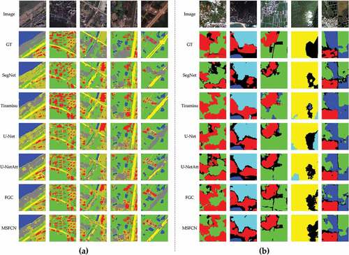
Table 4 summarizes the per class F1-score performance of the different methods for WHDLD and GID. The proposed MSFCN obtains the best performance in most classes on WHDLD and whole classes on GID. Meanwhile, we investigate the confusion between each pair of categories, and we report the confusion matrix by heat maps for each competing method in Figure 10. The more visible diagonal structure (the dark blue blocks concentrated on the diagonal) indicates the more powerful capacity of distinguishing between classes. And the diagonal structure of MSFCN is more distinct than others, which proves our framework’s superiority. Some visual results generated by our method and comparisons are provided in Figure 11.

Table 4. Per class F1-score performance on WHDLD and GID

Dataset	Method	bare	building	pavement	road	vegetable	water
WHDLD	SegNet	47.682	63.253	51.466	54.649	86.473	95.649
	Tiramisu	50.313	68.918	53.576	70.047	88.206	96.598
	U-Net	43.097	70.752	52.609	58.668	89.185	97.089
	U-NetAtt	47.974	72.736	48.942	60.576	89.994	97.511
	FGC	50.282	72.642	53.842	57.931	89.651	97.294
	MSFCN	52.178	74.499	55.177	68.797	90.024	97.511
GID	SegNet	63.451	79.085	83.510	89.241	84.962	93.493
	Tiramisu	57.062	79.007	85.436	87.068	83.274	92.449
	U-Net	63.351	80.585	81.564	87.768	82.996	91.692
	U-NetAtt	67.123	81.523	84.569	86.955	82.513	92.381
	FGC	66.810	81.957	84.101	89.570	84.840	92.165
	MSFCN	71.536	83.442	86.907	90.332	85.752	94.303

Figure 10. Heat maps of different methods on (a) WHDLD and (b) GID.

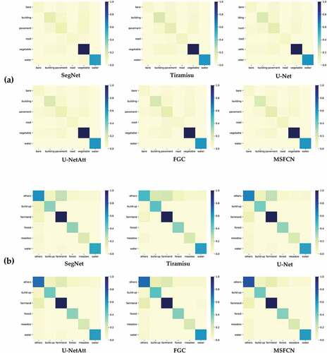
Figure 11. Land cover classification results of the method proposed and comparisons on (a) WHDLD and (b) GID.

The number of parameters and the calculations’ consumptions are also significant to assess a framework’s merit. The comparison of parameters and computational complexity between different algorithms are reported in Table 5, where “M” is the abbreviation of million, the unit of parameter number, and “G” is the abbreviation of Gillion (thousand million), the unit of floating point operations. And the comparison demonstrates that the design of MSFCN does not bring in redundant parameters or lead to high computational complexity.

Table 5. The comparison of parameters and computational complexity for 2D datasets, where “M” is the abbreviation of million, the unit of parameter number, and “G” is the abbreviation of Gillion (thousand million), the unit of floating point operations

Method	input shape	Parameters (M)	Complexity (G)
SegNet	3 × 256 × 256	1.93	9.27
Tiramisu		29.45	40.29
U-Net		1.38	11.92
U-NetAtt		2.17	12.75
FGC		2.19	8.4
MSFCN		2.67	9.66

3.4. Results on 2015 and 2017 datasets

To train the network, the inputs of the 1D U-Net are reshaped into $\left(\mathit{ct}\times 65,536\right)$ tensors, and the inputs of the 2D U-Net are reshaped into $\left(\mathit{ct}\times 256\times 256\right)$, while the inputs of the Conv-LSTM, 3D U-Net, 3D FGC, 3D U-NetAtt and 3D MSFCN are $\left(\mathit{c}\times \mathit{t}\times 256\times 256\right)$ tensors, where c and t denote the number of spectral channels and time series, respectively.

The experimental results with the different methods for two datasets are demonstrated in Table 6. Since 1D CNN’s operation destroys both the spatial and temporal dimensions, 1D U-Net’s performance is worst. As 2D CNN’s process ruins the temporal dimension when extracting spatio-temporal features, the models based on 3D CNN dramatically outperform the models based on 2D CNN, which prominently demonstrates the superiority of 3D CNN. The performance of Conv-LSTM transcends 2D-based models, as the information contained in the temporal dimension is taken into consideration. Benefitting from the utilization of attention mechanisms, the 3D U-NetAtt performs better than 3D U-Net.

Table 6. The experimental results using different methods on 2015 dataset and 2017 dataset

Dataset	Method	OA	AA	K	mIoU	FWIoU	F1
2015	1D U-Net	92.302	75.017	87.339	66.745	86.581	76.114
	2D U-Net	91.883	85.710	86.788	74.131	86.174	84.117
	3D U-Net	96.620	85.819	94.391	82.151	93.517	88.112
	3D U-NetAtt	96.272	90.662	93.876	83.441	93.143	88.947
	Conv-LSTM	96.682	90.314	94.523	84.618	93.770	91.123
	3D FGC	96.272	90.662	93.876	83.441	93.143	90.380
	3D MSFCN	97.784	93.275	96.339	87.753	95.848	92.971
2017	1D U-Net	95.709	74.331	89.365	66.091	92.065	75.924
	2D U-Net	96.369	78.015	90.933	71.873	93.491	81.449
	3D U-Net	96.662	81.836	91.851	74.375	94.252	83.497
	3D U-NetAtt	97.102	82.320	93.020	75.505	94.904	84.380
	Conv-LSTM	96.414	81.379	91.117	75.026	93.456	84.156
	3D FGC	97.083	82.052	92.841	75.387	94.767	84.311
	3D MSFCN	97.132	85.088	93.039	77.156	94.880	86.018

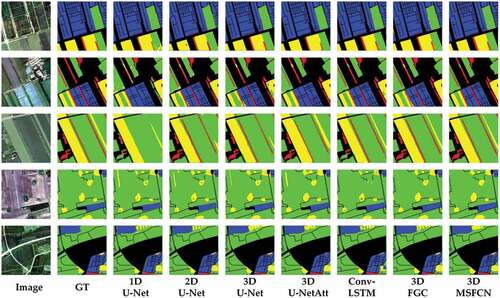
Similarly, FGC’s performance exceeds U-Net due to the consistency enhanced by CAB and GPM. Our proposed MSFCN obtains the state-of-the-art mIoU on two datasets, as the well-designed multi-scale convolutional blocks capture both the global and local features. Table 7 reports the per class F1-score performance of the different methods for the 2015 dataset and 2017 dataset. The proposed MSFCN obtains the best performance in whole classes on the 2015 dataset and most classes on the 2017 dataset. The confusion matrix reported by heat maps for each competing method is provided in Figure 12. And Figure 13 demonstrates the segmentation maps on two datasets. The first three rows are from the 2015 dataset, and the remainder is from the 2017 dataset. Taking the fourth column as an example, the proposed MSFCN differentiates corn (green) and grass (yellow) better than other models. Table 8 provides the number of parameters and the consumption of calculation, which illustrates the complexity of the proposed MSFCN is not unacceptable.

Table 7. Per class F1-score performance on 2015 dataset and 2017 dataset

Dataset	Method	rice	corn	sorghum	tree
2015	1D U-Net	97.743	92.968	75.965	37.781
	2D U-Net	97.301	92.321	72.225	74.623
	3D U-Net	98.476	95.780	82.997	75.194
	3D U-NetAtt	98.369	97.055	92.721	67.642
	Conv-LSTM	98.733	97.154	89.791	78.813
	3D FGC	98.670	96.839	87.997	78.013
	3D MSFCN	99.184	98.203	94.317	80.180
2017	1D U-Net	96.582	97.671	58.544	50.899
	2D U-Net	97.226	97.864	65.230	65.476
	3D U-Net	97.868	98.115	67.790	70.215
	3D U-NetAtt	97.752	98.413	74.264	67.091
	Conv-LSTM	96.643	97.940	65.798	76.244
	3D FGC	97.861	98.335	72.562	68.485
	3D MSFCN	98.236	98.586	77.660	69.589

Table 8. The comparison of parameters and computational complexity for 3D datasets, where “M” is the abbreviation of million, the unit of parameter number, and “G” is the abbreviation of Gillion (thousand million), the unit of floating point operations

Method	input shape	Parameters (M)	Complexity (G)
1D U-Net	16 × 65, 536	3.74	24.16
2D U-Net	16 × 256 × 256	10.86	14.18
3D U-Net	4 × 4 × 256 × 256	4.87	74.69
3D U-NetAtt		5.67	121.74
Conv-LSTM		0.30	77.31
3D FGC		5.32	78.51
3D MSFCN		6.58	91.46

Figure 12. Heat maps of different methods on (a) 2015 and (b) 2017 datasets.

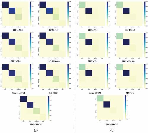
Figure 13. Land cover classification results of the method proposed and comparisons on the 2015 dataset and 2017 dataset, where the first three rows are from the 2015 dataset, and the remainder is from the 2017 dataset.

3.5. Effectiveness of the Multi-Scale Convolutional Block and attention mechanisms

We verified the effectiveness of the multi-scale convolutional block and attention mechanisms in this section. Concretely, we analyzed the proposed MSFCN without Multi-Scale Convolutional Block (MSFB), Channel Attention Block (CAB), and Global Pooling Module (GPM) both on WHDLD and GID. The results are shown in Table 9.

Table 9. The effectiveness of the Multi-Scale Convolutional Block and attention mechanisms on WHDLD and GID

Dataset	Method	OA	AA	K	mIoU	FWIoU	F1
WHDLD	U-Net	81.830	67.724	74.422	55.706	72.450	68.567
	MSFB	82.708	68.301	75.459	57.098	73.119	69.941
	MSFB+CAB	83.084	70.411	76.038	58.571	73.547	71.299
	MSFB+GPM	83.433	70.214	76.608	58.608	74.347	71.003
	MSFCN	84.168	72.081	77.558	60.366	74.892	73.031
GID	U-Net	78.992	81.115	73.295	69.417	65.936	81.326
	MSFB	81.579	83.429	76.620	71.992	69.715	83.276
	MSFB+CAB	82.675	84.693	78.111	73.672	70.987	84.321
	MSFB+GPM	82.891	84.136	78.302	73.671	71.575	84.453
	MSFCN	83.718	85.544	79.353	75.127	72.688	85.378

The 3D U-Net obtains mIoU of 55.706% and 69.417% on WHDLD and GID, respectively. By utilizing multi-scale convolutional blocks, the mIoUs reach 57.098%, and 71.992%. And the introduction of channel attention block and global pooling module brings 1.473%/1.510% for WHDLD and 1.680%/1.679% for GID improvements on mIoU, respectively. The mIoUs are further improved to 60.366% and 75.127% when all blocks are introduced.

3.6. Investigation about the number of layers and channels

The number of layers and channels are two vital parameters that impact the model’s performance and determine the computational complexity. Thus, it is worthwhile to investigate the influence of the number of layers and channels.

Therefore, we implemented experiments to inquire about the effect caused by the number of layers. Concretely, we design an MSFCN with 3 layers (MSFCN3) and an MSFCN with 5 layers (MSFCN5) and compare their performance with the MSFCN with the proposed 4 layers MSFCN (MSFCN4). As finite layers limit the capacity of representations, the performance of MSFCN3 is significantly weaker than MSFCN4. Specifically, without enormous increases in the parameters and computational complexity, MSFCN4 surpasses MSFCN3 more than 5% on mIoU, seen in Table 10. However, notwithstanding the certain improvements boosted by MSFCN5, the number of parameters of MSFCN5 is four times more than MSFCN4’s (Table 11), which is not an efficient option.

Table 10. The comparison between the number of layers and the number of channels on the GID dataset

Factor	Method	OA	AA	K	mIoU	FWIoU	F1
Layers	MSFCN3	79.513	80.862	74.178	69.858	67.243	81.723
	MSFCN4	83.718	85.544	79.353	75.127	72.688	85.378
	MSFCN5	84.449	86.554	80.300	76.042	73.843	86.010
Channels	MSFCNN	80.218	83.652	70.530	70.530	67.529	82.104
	MSFCN	83.718	85.544	79.353	75.127	72.688	85.378
	MSFCNW	84.352	86.966	80.230	75.669	73.365	85.733

Table 11. The comparison of parameters and computational complexity for variants of MSFCN, where “M” is the abbreviation of million, the unit of parameter number, and “G” is the abbreviation of Gillion (thousand million), the unit of floating point operations

Method	input shape	Parameters (M)	Complexity (G)
MSFCN3	3 × 256 × 256	2.52	6.77
MSFCN4		2.67	9.66
MSFCN5		10.73	12.55
MSFCNN	3 × 256 × 256	0.67	2.46
MSFCN		2.67	9.66
MSFCNW		10.65	38.24

Besides, we designed experiments to research the impact caused by the number of channels. Specifically, we designed a narrow MSFCN (MSFCNN) with [16, 32, 64, 128] channels, and a wide MSFCN (MSFCNW) with [64, 128, 256, 512] channels, and compare their performance with the proposed MSFCN with [32, 64, 128, 256] channels. The results in Table 10 show that the performance of MSFCN surpasses MSFCNN near 5% on mIoU. Meanwhile, with five times on parameters and computational complexity, MSFCNW just brings nearly a 1% improvement. Based on the above experiments, we can conclude that the proposed MSFCN delicately balances the performance and complexity.

4. Conclusions

In this paper, to implement land cover classification using satellite images, we propose a Multi-Scale Fully Convolutional Network (MSFCN). Firstly, multi-scale convolutional blocks are elaborately designed to expand the scope of information extraction in the spatial domain, capturing both the satellite images’ local and global information. Secondly, a channel attention block and a global pooling module enhance channel consistency and global contextual consistency. Thirdly, we extend MSFCN to 3D for spatio-temporal satellite images based on 3D CNN to replace 2D FCN, which adequately utilizes each land cover class’s time series interaction on the temporal dimension. Extensive experiments demonstrate that the proposed MSFCN, with the performance and complexity well balanced, is not only comparative with the baseline on spatial images but also effective on spatio-temporal images. And experiment results also show that the 3D CNN is significantly superior to 2D CNN on land cover classification for spatio-temporal images.

Our future directions include two major aspects: the first one is to construct a more complex scenario with easily-confused land covers to further verify the effectiveness of the proposed MSFCN; the second one is to explore the more elaborate structure such as 3D-ResNet for land cover classification of spatio-temporal images to enhance the representation capacity of the network, thereby better distinguishing the easily confusing targets.

Disclosure statement

No potential conflict of interest was reported by the author(s).

Data availability statement

The data used to support the findings of this study are included within the article.

WHDLD:https://sites.google.com/view/zhouwx/dataset?authuser=0#h.p_ebsAS1Bikmkd

GID:https://x-ytong.github.io/project/GID.html

2015&2017:http://gpcv.whu.edu.cn/data/3DFGC_pages.html

Additional information

Funding

This work is supported by the National Natural Science Foundation of China [grant number 41671452].

Notes on contributors

Rui Li

Rui Li is currently pursuing a master’s degree at Wuhan University. His research interests include semantic segmentation, hyperspectral image classification, and deep learning.

Shunyi Zheng

Shunyi Zheng received the Post-Doctorate from Wuhan University in 2002 and is currently a Professor there. His research interests include remote sensing data processing, digital photogrammetry, and three-dimensional reconstruction. Prof. Zheng received the First Prize for Scientific and Technological Progress in Surveying and Mapping, China, in 2012 and 2019.

Chenxi Duan

Chenxi Duan is currently pursuing a Ph.D. degree in the Faculty of Geo-Information Science and Earth Observation (ITC) at the University of Twente. Her research interests include remote sensing image processing, cloud removal, and numerical optimization.

Libo Wang

Libo Wang is currently pursuing a Ph.D. degree at Wuhan University. His research interests include computer vision and remote sensing image analysis.

Ce Zhang

Ce Zhang received a Ph.D. Degree in Geography from Lancaster Environment Centre, Lancaster University, U.K. in 2018. He was the recipient of a prestigious European Union (EU) Erasmus Mundus Scholarship for a European Joint MSc programme between the University of Twente (The Netherlands) and the University of Southampton (U.K.). Dr. Zhang is currently a Lecturer in Geospatial Data Science at the Centre of Excellence in Environmental Data Science (CEEDS), jointly venture between Lancaster University and UK Centre for Ecology & Hydrology (UKCEH). His major research interests include geospatial artificial intelligence, machine learning, deep learning, and remotely sensed image analysis.

References

- Badrinarayanan, V., A. Kendall, and R. Cipolla. 2017. “SegNet: A Deep Convolutional Encoder-Decoder Architecture for Image Segmentation.” IEEE Transactions on Pattern Analysis and Machine Intelligence 39 (12): 2481–2495. doi:10.1109/TPAMI.2016.2644615.
- Basso, B., and L. Liu. 2019. “Seasonal Crop Yield Forecast: Methods, Applications, and Accuracies.” In Advances in Agronomy, 201–255. Cambridge, MA: Elsevier.
- Chen, L.-C., Y. Zhu, G. Papandreou, F. Schroff, and H. Adam. 2018. “Encoder-Decoder with Atrous Separable Convolution for Semantic Image Segmentation.” 15th European Conference on Computer Vision (ECCV), Munich, Germany, September 8–14.
- Chen, L., J. Liu, H. Li, W. Zhan, B. Zhou, and Q. Li. 2020. “Dual Context Prior and Refined Prediction for Semantic Segmentation.” Geo-Spatial Information Science 1–13. doi:10.1080/10095020.2020.1785957.
- Dela Torre, D.M.G., J. Gao, and C. Macinnis-Ng. 2021. “Remote Sensing-based Estimation of Rice Yields Using Various Models: A Critical Review.” Geo-spatial Information Science 1–24. doi:10.1080/10095020.2021.1936656.
- Du, Q., and I.C. Chein. 2001. “A Linear Constrained Distance-based Discriminant Analysis for Hyperspectral Image Classification.” Pattern Recognition 34 (2): 361–373. doi:10.1016/S0031-3203(99)00215-0.
- Duan, C., J. Pan, and R. Li. 2020. “Thick Cloud Removal of Remote Sensing Images Using Temporal Smoothness and Sparsity Regularized Tensor Optimization.” Remote Sensing 12 (20): 3446(3426). doi:10.3390/rs12203446.
- Gao, B.-C. 1996. “NDWI—A Normalized Difference Water Index for Remote Sensing of Vegetation Liquid Water from Space.” Remote Sensing of Environment 58 (3): 257–266. doi:10.1016/S0034-4257(96)00067-3.
- Georganos, S., T. Grippa, S. Vanhuysse, M. Lennert, M. Shimoni, and E. Wolff. 2018. “Very High Resolution Object-Based Land Use-Land Cover Urban Classification Using Extreme Gradient Boosting.” IEEE Geoscience and Remote Sensing Letters 15 (4): 607–611. doi:10.1109/LGRS.2018.2803259.
- Gong, Z., H. Lin, D. Zhang, Z. Luo, J. Zelek, Y. Chen, A. Nurunnabi, C. Wang, and J. Li. 2020. “A Frustum-based Probabilistic Framework for 3D Object Detection by Fusion of LiDAR and Camera Data.” ISPRS Journal of Photogrammetry and Remote Sensing 159: 90–100. doi:10.1016/j.isprsjprs.2019.10.015.
- Hamraz, H., N.B. Jacobs, M.A. Contreras, and C.H. Clark. 2019. “Deep Learning for Conifer/deciduous Classification of Airborne LiDAR 3D Point Clouds Representing Individual Trees.” ISPRS Journal of Photogrammetry and Remote Sensing 158: 219–230. doi:10.1016/j.isprsjprs.2019.10.011.
- Heipke, C., and F. Rottensteiner. 2020. “Deep Learning for Geometric and Semantic Tasks in Photogrammetry and Remote Sensing.” Geo-spatial Information Science 23 (1): 10–19. doi:10.1080/10095020.2020.1718003.
- Huete, A. 1988. “A Soil-adjusted Vegetation Index (SAVI). Remote Sensing of Environment.” Remote Sensing of Environment 25: 295–309. doi:10.1016/0034-4257(88)90106-X.
- Interdonato, R., D. Ienco, R. Gaetano, and K. Ose. 2019. “DuPLO: A DUal View Point Deep Learning Architecture for Time Series classificatiOn.” ISPRS Journal of Photogrammetry and Remote Sensing 149: 91–104. doi:10.1016/j.isprsjprs.2019.01.011.
- Ioffe, S., and C. Szegedy. 2015. “Batch Normalization: Accelerating Deep Network Training by Reducing Internal Covariate Shift.” arXiv Preprint arXiv:1502.03167.
- Jegou, S., M. Drozdzal, D. Vazquez, A. Romero, and Y. Bengio. 2017. “The One Hundred Layers Tiramisu: Fully Convolutional DenseNets for Semantic Segmentation.” 2017 IEEE Conference on Computer Vision and Pattern Recognition: Workshops (CVPRW), Loa Alamitos, CA, July 21–26.
- Ji, S., C. Zhang, A. Xu, Y. Shi, and Y. Duan. 2018. “3D Convolutional Neural Networks for Crop Classification with Multi-temporal Remote Sensing Images.” Remote Sensing 10 (1): 75. doi:10.3390/rs10010075.
- Ji, S., Z. Zhang, C. Zhang, S. Wei, M. Lu, and Y. Duan. 2020. “Learning Discriminative Spatiotemporal Features for Precise Crop Classification from Multi-temporal Satellite Images.” International Journal of Remote Sensing 41 (8): 3162–3174. doi:10.1080/01431161.2019.1699973.
- Li, H., C. Wang, C. Zhong, A. Su, C. Xiong, J. Wang, and J. Liu. 2017. “Mapping Urban Bare Land Automatically from Landsat Imagery with a Simple Index.” Remote Sensing 9 (3): 249. doi:10.3390/rs9030249.
- Li, R., C. Duan, S. Zheng, C. Zhang, and P.M. Atkinson. 2021a. “MACU-Net for Semantic Segmentation of Fine-Resolution Remotely Sensed Images.” IEEE Geoscience and Remote Sensing Letters. doi:10.1109/LGRS.2021.3052886.
- Li, R., S. Zheng, C. Duan, J. Su, and C. Zhang. 2021b. “Multistage Attention ResU-Net for Semantic Segmentation of Fine-Resolution Remote Sensing Images.” IEEE Geoscience and Remote Sensing Letters. doi:10.1109/LGRS.2021.3063381.
- Li, R., S. Zheng, C. Duan, Y. Yang, and X. Wang. 2020. “Classification of Hyperspectral Image Based on Double-Branch Dual-Attention Mechanism Network.” Remote Sensing 12 (3): 582. doi:10.3390/rs12030582.
- Li, R., S. Zheng, C. Zhang, C. Duan, J. Su, L. Wang, and P.M. Atkinson. 2021d. “Multiattention Network for Semantic Segmentation of Fine-Resolution Remote Sensing Images.” IEEE Transactions on Geoscience and Remote Sensing. doi:10.1109/TGRS.2021.3093977.
- Li, R., S. Zheng, C. Zhang, C. Duan, L. Wang, and P.M. Atkinson. 2021c. “ABCNet: Attentive Bilateral Contextual Network for Efficient Semantic Segmentation of Fine-Resolution Remotely Sensed Imagery.” ISPRS Journal of Photogrammetry and Remote Sensing 181: 84–98. doi:10.1016/j.isprsjprs.2021.09.005.
- Li, Z., L. Jiao, B. Zhang, G. Xu, and J. Liu. 2021e. “Understanding the Pattern and Mechanism of Spatial Concentration of Urban Land Use, Population and Economic Activities: A Case Study in Wuhan, China.” Geo-spatial Information Science 1–17. doi:10.1080/10095020.2021.1978276.
- Liu, Q., M. Kampffmeyer, R. Jenssen, and A.-B. Salberg. 2020. “Dense Dilated Convolutions’ Merging Network for Land Cover Classification.” IEEE Transactions on Geoscience and Remote Sensing 58 (9): 6309–6320. doi:10.1109/TGRS.2020.2976658.
- Liu, W., A. Rabinovich, and A.C. Berg. 2015. “Parsenet: Looking Wider to See Better.” arXiv Preprint arXiv:1506.04579.
- Matikainen, L., K. Karila, J. Hyyppa, P. Litkey, E. Puttonen, and E. Ahokas. 2017. “Object-based Analysis of Multispectral Airborne Laser Scanner Data for Land Cover Classification and Map Updating.” ISPRS Journal of Photogrammetry and Remote Sensing 128: 298–313. doi:10.1016/j.isprsjprs.2017.04.005.
- Maulik, U., and I. Saha. 2010. “Automatic Fuzzy Clustering Using Modified Differential Evolution for Image Classification.” IEEE Transactions on Geoscience and Remote Sensing 48 (9): 3503–3510. doi:10.1109/TGRS.2010.2047020.
- Mohammadimanesh, F., B. Salehi, M. Mahdianpari, E. Gill, and M. Molinier. 2019. “A New Fully Convolutional Neural Network for Semantic Segmentation of Polarimetric SAR Imagery in Complex Land Cover Ecosystem.” ISPRS Journal of Photogrammetry and Remote Sensing 151: 223–236. doi:10.1016/j.isprsjprs.2019.03.015.
- Oktay, O., J. Schlemper, L.L. Folgoc, M. Lee, M. Heinrich, K. Misawa, K. Mori, S. McDonagh, N.Y. Hammerla, and B. Kainz. 2018. “Attention U-net: Learning Where to Look for the Pancreas.” arXiv Preprint arXiv:1804.03999.
- Pelletier, C., G.I. Webb, and F. Petitjean. 2019. “Temporal Convolutional Neural Network for the Classification of Satellite Image Time Series.” Remote Sensing 11 (5): 523. doi:10.3390/rs11050523.
- Prins, A.J., and A. Van Niekerk. 2020. “Crop Type Mapping Using LiDAR, Sentinel-2 and Aerial Imagery with Machine Learning Algorithms.” Geo-Spatial Information Science 1–13. doi:10.1080/10095020.2020.1782776.
- Qi, Y., S. Chodron Drolma, X. Zhang, J. Liang, H. Jiang, J. Xu, and T. Ni. 2020. “An Investigation of the Visual Features of Urban Street Vitality Using a Convolutional Neural Network.” Geo-spatial Information Science 23 (4): 341–351. doi:10.1080/10095020.2020.1847002.
- Ramli, M.F., and K.N. Tahar. 2020. “Homogeneous Tree Height Derivation from Tree Crown Delineation Using Seeded Region Growing (SRG) Segmentation.” Geo-spatial Information Science 23 (3): 195–208. doi:10.1080/10095020.2020.1805366.
- Ronneberger, O., P. Fischer, and T. Brox. 2015. “U-Net: Convolutional Networks for Biomedical Image Segmentation.” Medical Image Computing and Computer-Assisted Intervention - MICCAI 2015. 18th International Conference, Munich, Germany, October 5–9.
- Rußwurm, M., and M. Körner. 2018. “Multi-temporal Land Cover Classification with Sequential Recurrent Encoders.” ISPRS International Journal of Geo-Information 7 (4): 129. doi:10.3390/ijgi7040129.
- Rustowicz, R., R. Cheong, L. Wang, S. Ermon, M. Burke, and D. Lobell. 2019. “Semantic Segmentation of Crop Type in Africa: A Novel Dataset and Analysis of Deep Learning Methods.” 32nd IEEE/CVF Conference on Computer Vision and Pattern Recognition Workshops, CVPRW 2019, Long Beach, CA, June 16–20.
- Rutherford, G., A. Guisan, and N. Zimmermann. 2007. “Evaluating Sampling Strategies and Logistic Regression Methods for Modelling Complex Land Cover Changes.” Journal of Applied Ecology 44 (2): 414–424. doi:10.1111/j.1365-2664.2007.01281.x.
- Sainte Fare Garnot, V., L. Landrieu, S. Giordano, and N. Chehata. 2020. “Satellite Image Time Series Classification with Pixel-Set Encoders and Temporal Self-Attention.” 2020 IEEE/CVF Conference on Computer Vision and Pattern Recognition (CVPR), Los Alamitos, CA, June 13–19.
- Sang, Q., Y. Zhuang, S. Dong, G. Wang, and H. Chen. 2019. “FRF-Net: Land Cover Classification from Large-scale VHR Optical Remote Sensing Images.” IEEE Geoscience and Remote Sensing Letters 17 (6): 1057–1061. doi:10.1109/LGRS.2019.2938555.
- Shao, Z., W. Wu, and D. Li. 2021. “Spatio-temporal-spectral Observation Model for Urban Remote Sensing.” Geo-spatial Information Science 1–15. doi:10.1080/10095020.2020.1864232.
- Shao, Z., W. Zhou, X. Deng, M. Zhang, and Q. Cheng. 2020. “Multilabel Remote Sensing Image Retrieval Based on Fully Convolutional Network.” IEEE Journal of Selected Topics in Applied Earth Observations and Remote Sensing 13: 318–328. doi:10.1109/JSTARS.2019.2961634.
- Tatsumi, K., Y. Yamashiki, M.A.C. Torres, and C.L.R. Taipe. 2015. “Crop Classification of Upland Fields Using Random Forest of Time-series Landsat 7 ETM+ Data.” Computers and Electronics in Agriculture 115: 171–179. doi:10.1016/j.compag.2015.05.001.
- Tong, X.-Y., G.-S. Xia, Q. Lu, H. Shen, S. Li, S. You, and L. Zhang. 2020. “Land-cover Classification with High-resolution Remote Sensing Images Using Transferable Deep Models.” Remote Sensing of Environment 237: 111322. doi:10.1016/j.rse.2019.111322.
- Tucker, C.J. 1979. “Red and Photographic Infrared Linear Combinations for Monitoring Vegetation.” Remote Sensing of Environment 8 (2): 127–150. doi:10.1016/0034-4257(79)90013-0.
- Wang, G., J. Li, W. Sun, B. Xue, A. Yinglan, and T. Liu. 2019a. “Non-point Source Pollution Risks in a Drinking Water Protection Zone Based on Remote Sensing Data Embedded within a Nutrient Budget Model.” Water Research 157: 238–246. doi:10.1016/j.watres.2019.03.070.
- Wang, L., R. Li, C. Duan, C. Zhang, X. Meng, and S. Fang. 2021a. “A Novel Transformer Based Semantic Segmentation Scheme for Fine-Resolution Remote Sensing Images.” arXiv Preprint arXiv:2104.12137.
- Wang, L., R. Li, D. Wang, C. Duan, T. Wang, and X. Meng. 2021b. “Transformer Meets Convolution: A Bilateral Awareness Network for Semantic Segmentation of Very Fine Resolution Urban Scene Images.” Remote Sensing 13 (16). doi:10.3390/rs13163065.
- Wang, P., L. Zhang, G. Zhang, H. Bi, M. Dalla Mura, and J. Chanussot. 2019b. “Superresolution Land Cover Mapping Based on Pixel-, Subpixel-, and Superpixel-scale Spatial Dependence with Pansharpening Technique.” IEEE Journal of Selected Topics in Applied Earth Observations and Remote Sensing 12 (10): 4082–4098. doi:10.1109/JSTARS.2019.2939670.
- Wu, C.-Y., C. Feichtenhofer, H. Fan, K. He, P. Krahenbuhl, and R. Girshick. 2019. “Long-Term Feature Banks for Detailed Video Understanding.” 2019 IEEE/CVF Conference on Computer Vision and Pattern Recognition (CVPR), Los Alamitos, CA, June 15–20.
- Wu, H., Z. Gui, and Z. Yang. 2020. “Geospatial Big Data for Urban Planning and Urban Management.” Geo-Spatial Information Science 23 (4): 273–274. doi:10.1080/10095020.2020.1854981.
- Xu, H. 2006. “Modification of Normalised Difference Water Index (NDWI) to Enhance Open Water Features in Remotely Sensed Imagery.” International Journal of Remote Sensing 27 (14): 3025–3033. doi:10.1080/01431160600589179.
- Yang, C., Q. Zhan, S. Gao, and H. Liu. 2020. “Characterizing the Spatial and Temporal Variation of the Land Surface Temperature Hotspots in Wuhan from a Local Scale.” Geo-spatial Information Science 23 (4): 327–340. doi:10.1080/10095020.2020.1834882.
- Yu, C., J. Wang, C. Peng, C. Gao, G. Yu, and N. Sang. 2018. “BiSeNet: Bilateral Segmentation Network for Real-Time Semantic Segmentation.” Computer Vision. 15th European Conference (ECCV 2018), Munich, Germany, September 8–14.
- Zafari, A., R. Zurita-Milla, and E. Izquierdo-Verdiguier. 2020. “Land Cover Classification Using Extremely Randomized Trees: A Kernel Perspective.” IEEE Geoscience and Remote Sensing Letters 17 (10): 1702–1706. doi:10.1109/LGRS.2019.2953778.
- Zhang, C., X. Pan, H. Li, A. Gardiner, I. Sargent, J. Hare, and P.M. Atkinson. 2018. “A Hybrid MLP-CNN Classifier for Very Fine Resolution Remotely Sensed Image Classification.” ISPRS Journal of Photogrammetry and Remote Sensing 140: 133–144. doi:10.1016/j.isprsjprs.2017.07.014.
- Zhang, C., Y. Han, F. Li, S. Gao, D. Song, H. Zhao, K. Fan, and Y.N. Zhang. 2019a. “A New CNN-Bayesian Model for Extracting Improved Winter Wheat Spatial Distribution from GF-2 Imagery.” Remote Sensing 11 (6): 619. doi:10.3390/rs11060619.
- Zhang, J., L. Feng, and F. Yao. 2014. “Improved Maize Cultivated Area Estimation over a Large Scale Combining MODIS–EVI Time Series Data and Crop Phenological Information.” ISPRS Journal of Photogrammetry and Remote Sensing 94: 102–113. doi:10.1016/j.isprsjprs.2014.04.023.
- Zhang, Z., Y. Liu, T. Liu, Z. Lin, and S. Wang. 2019b. “DAGN: A Real-time UAV Remote Sensing Image Vehicle Detection Framework.” IEEE Geoscience and Remote Sensing Letters 17 (11): 1884–1888. doi:10.1109/LGRS.2019.2956513.
- Zhao, H., and X. Chen. 2005. “Use of Normalized Difference Bareness Index in Quickly Mapping Bare Areas from TM/ETM+.” 2005 IEEE International Geoscience and Remote Sensing Symposium, IGARSS 2005, Seoul, Korea, July 25–29.
- Zhong, L., L. Hu, and H. Zhou. 2019. “Deep Learning Based Multi-temporal Crop Classification.” Remote Sensing of Environment 221: 430–443. doi:10.1016/j.rse.2018.11.032.
- Zhong, Y., A. Ma, Y. Soon Ong, Z. Zhu, and L. Zhang. 2018. “Computational Intelligence in Optical Remote Sensing Image Processing.” Applied Soft Computing 64: 75–93. doi:10.1016/j.asoc.2017.11.045.