An optimal design of the broadcast ephemeris for LEO navigation augmentation systems

ABSTRACT

As the deployment of large Low Earth Orbiters (LEO) communication constellations, navigation from the LEO satellites becomes an emerging opportunity to enhance the existing satellite navigation systems. The LEO navigation augmentation (LEO-NA) systems require a centimeter to decimeter accuracy broadcast ephemeris to support high accuracy positioning applications. Thus, how to design the broadcast ephemeris becomes the key issue for the LEO-NA systems. In this paper, the temporal variation characteristics of the LEO orbit elements were analyzed via a spectrum analysis. A non-singular element set for orbit fitting was introduced to overcome the potential singularity problem of the LEO orbits. Based on the orbit characteristics, a few new parameters were introduced into the classical 16 parameter ephemeris set to improve the LEO orbit fitting accuracy. In order to identify the optimal parameter set, different parameter sets were tested and compared and the 21 parameters data set was recommended to make an optimal balance between the orbit accuracy and the bandwidth requirements. Considering the real-time broadcast ephemeris generation procedure, the performance of the LEO ephemeris based on the predicted orbit is also investigated. The performance of the proposed ephemeris set was evaluated with four in-orbit LEO satellites and the results indicate the proposed 21 parameter schemes improve the fitting accuracy by 87.4% subject to the 16 parameters scheme. The accuracy for the predicted LEO ephemeris is strongly dependent on the orbit altitude. For these LEO satellites operating higher than 500 km, 10 cm signal-in-space ranging error (SISRE) is achievable for over 20 min prediction.

KEYWORDS:

• LEO
• broadcast ephemeris
• orbit fitting
• leo navigation augmentation
• orbit prediction

1. Introduction

In recent years, the applications of Low Earth Orbiters (LEO) have attracted increasing attention in communication and navigation applications (Wang and El-Mowafy 2021; Parkinson 2014; Reid et al. 2020). A few mega LEO constellations plan has been proposed to provide global, low latency communication service, which also brings new opportunities for navigation applications. Current satellite navigation systems are all based on the Medium Earth Orbiters (MEO) or higher satellites, which have slow geometry variation and weak signals. The fast geometry change of the LEO satellite can dramatically improve the convergence time of precise positioning applications. By integrating with the communication satellites, the corrections of Global Navigation Satellite Systems (GNSS) signals can be transmitted everywhere on the earth to provide precise positioning services (Tian, Zhang, and Bian 2019; Wang et al. 2020b; Sun et al. 2016; Ge et al. 2021). In addition, the integration of the LEO communication and navigation service is a promising solution to solve the precious frequency resources and improve the resilience of the existing Positioning, Navigation, and Timing (PNT) services (Li, Jiang, and Dong 2020; Chen et al. 2019). The LEO Navigation Augmentation (LEO-NA) system is targeting to enhance the service capacity of the existing GNSS and provide globally, real-time precise positioning services and more resilience and secured PNT services(Yang 2016; Li et al. 2018, 2019). Recently, several in-orbit LEO-NA experiments have demonstrated the benefit of navigation augmentation from LEO satellites, such as the Luojia-1A satellite developed by Wuhan University (Wang et al. 2018, 2019, 2020a).

The precise broadcast ephemeris is the prerequisite for real-time precise positioning, while the dynamic condition for most LEO satellites is more complex than the GNSS satellites. Hence, it is a new challenge to design the LEO broadcast ephemeris to support real-time precise positioning applications. The GNSS broadcast ephemeris fitting algorithms have been extensively studied and the 16-parameter scheme based on the Keplerian elements is the most popular broadcast ephemeris form for its efficiency. Xiao et al. used the Expectation-Maximization (EM) algorithm to investigate the impact of introducing two new parameters on the satellite ephemeris precision (Xiao 2013; Xiao et al. 2014, 2016). Huang et al. proposed a feasible solution to establish the broadcast ephemeris model in a hybrid constellation navigation system (Huang 2012). Wang et al. solved the singularity problem of the BeiDou GEO satellites using the Givens orthogonal transformation method (Wang 2014). Fu et al. proposed the Broadcast Ephemeris Parameter Set (BEPS) concept and presented an improved broadcast ephemeris scheme for different types of Beidou satellites based on simulation (Fu and Wu 2012). Du et al. proposed an improved 18-parameter broadcast ephemeris that solves the orbit singularity problem of GEO satellites in orbit determination (Du et al. 2015). Jin et al. improved the GEO/IGSO Navigation Satellites user algorithm by introducing a few parameters and they also analyzed the influence of range error due to truncation (RET) (Choi et al. 2020).

In contrast, the LEO broadcast ephemeris fitting problem has not attracted enough attention (Meng et al. 2021). Fang et al. analyzed the orbit dynamics of LEO satellites and designed a 16/18 parameter fitting algorithm, which successfully solved the small eccentricity singularity problem. They also attempted to design a tabular type and a Keplerian type broadcast ephemeris for the LEO broadcast ephemeris model (Fang 2017; Fang et al. 2019). Xie et al. attempted to improve the accuracy of the LEO broadcast ephemeris by introducing a few more parameters to the ephemeris (Xie et al. 2018). They tested three improved ephemeris schemes, namely 18-parameter, 20-parameter, and 22-parameter, and the 20-parameter set is recommended based on the simulation results.

However, there are still a few issues in the LEO ephemeris fitting never being touched. At first, the optimal parameter set has not been identified. The existing research mostly introduces the new parameters according to personal experience rather than orbit analysis. Hence, it is difficult to identify the optimal parameter set for the LEO ephemeris design. The second issue is the real-time broadcast ephemeris generation issue in practice has not been fully addressed since current research only focuses on the orbit fitting. The LEO ephemeris should be fitted based on a predicted orbit to provide real-time service; the orbit prediction error is also a major error source for the LEO ephemeris. The current ephemeris fitting algorithm only considers the fitting error, which may lead to an over-optimistic evaluation of the ephemeris accuracy. This study selected the extended LEO broadcast ephemeris parameter set based on LEO satellite orbital characteristic analysis. The optimal LEO Keplerian type broadcast ephemeris is proposed by a careful examination.

The remainder of the paper is organized as follows. Section 2 addressed the extended parameter set for LEO broadcast ephemeris based on the LEO orbit analysis. Section 3 introduced the user algorithms for the extended ephemeris. Section 4 evaluated the performance of different parameter sets and discussed several issues in parameter fitting. Section 5 discussed the issues related to parameter fitting with predicted orbit and Section 6 gives the conclusions.

2. Characteristics of the LEO orbit

The classical Keplerian type GNSS broadcast ephemeris comprises six basic Keplerian elements and nine perturbed parameters. Combined with the reference time $t_{oe}$, it was known as the 16 parameter ephemeris. The six Keplerian elements are given as orbital semi-major axis $a$, orbital eccentricity $e$, orbital inclination $i$, right ascension of the ascending node $\mathrm{\Omega }$, the argument of perigee $\omega$, and mean anomaly of the reference ephemeris $M$ (Misra and Enge 2006). These elements not only describe the motion status of the satellite but also include the orbit information. The satellite position can be simply expressed with four fundamental elements, given as the radial distance $r$, the orbit inclination $i$, the right ascension $\mathrm{\Omega }$ and the argument of latitude $u$. The relationship of these four elements is illustrated in Figure 1.

Figure 1. Illustration of the four basic orbit elements.

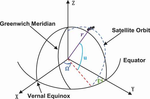
The position of the satellite in the ECEF coordinate system can be expressed with:

(1) $\left[\begin{array}{c}{X}_k\\ Y_k\\ Z_k\end{array}\right]=R_3\left(-\mathrm{\Omega }\right)\ast R_3\left(-i\right)\ast R_3\left(-u\right)\ast \left[\begin{array}{c}r\\ 0\\ 0\end{array}\right]$(1)

The argument of latitude $u$ can be computed from three Keplerian elements: the semi-major axis $a$, the eccentricity $e$ and the mean anomaly $M$. The reduced element set provides a more direct way to analyze the orbit characteristics. The classical GPS ephemeris also employs the reduced 4-parameter set as the intermedium parameter in the satellite position calculation process. In this study, the LEO orbit analysis is based on the reduced element set.

2.1. Harmonic analysis of LEO satellite orbit elements

LEO orbit representation method is similar to the navigation satellites, but its orbit characteristics are more complex. The GPS Legacy Navigation Message (LNAV) introduced six harmonic coefficients to the radial distance $r$, the argument of latitude $u$, and orbital inclination $i$. According to our experience, these parameters may not enough for the LEO satellites since the force model of LEO is more complicated. The sources of perturbation force experienced by low-orbit satellites in orbit mainly include the earth’s non-spherical gravity, third-body gravity, atmospheric resistance, solar radiation pressure, earth albedo pressure, tidal deformation, and post-Newton effect (Dong et al. 2016).

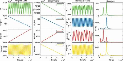
In order to find the best representation of the LEO orbit, harmonic analysis of the four orbit elements is performed and the results are presented in Figure 2. In the analysis, the variation of the four elements can be characterized as the sum of a linear trend and harmonic terms. A spectrum analysis further identified the periods of the harmonic terms. The results indicate that all four elements have multiple harmonic components, so it is not reasonable to follow the GPS LNAV design for the LEO ephemeris design. In the GPS LNAV, the changing rate of the radial range $r$ and the argument of latitude $\mathrm{u}$ are not considered. According to the harmonic analysis results, 18 harmonic terms can be introduced into the LEO ephemeris if all the periodical terms are considered, and they are listed as below: $C_{rs1},C_{rc1},C_{rs2},C_{rc2},C_{us1},C_{uc1},C_{us2},C_{uc2},C_{us3},C_{uc3},C_{is1},$ $C_{ic1},C_{is2},C_{ic2},C_{\mathrm{\Omega }s1},C_{\mathrm{\Omega }c1},C_{\mathrm{\Omega }s3},C_{\mathrm{\Omega }c3}$ where $C_{rs1},C_{rc1},C_{rs2},C_{rc2}$ are the amplitude of the harmonic perturbations for radial range, $C_{us1}$, $C_{uc1}$, $C_{us2},C_{uc2},C_{us3},C_{uc3}$ are the amplitude of the harmonic perturbations for the argument of latitude, and $C_{\mathrm{\Omega }s1},C_{\mathrm{\Omega }c1},C_{\mathrm{\Omega }s3},C_{\mathrm{\Omega }c3}$ are the amplitude of the harmonic perturbations for the right ascension of the ascending node.

Figure 2. Harmonic analysis results of the 4 basic orbit elements for JASON-2 satellite.

However, it is not reasonable to introduce all the observed terms into the ephemeris in practice for the following reason: (1) Some harmonic terms have a very small impact on the orbit precision, so they should not be considered in ephemeris fitting to save bandwidth. (2) In the four basic elements set, the right ascension $\mathrm{\Omega }$ is not perpendicular to the rest three elements, so introducing certain elements may have an impact on other harmonic terms. (3) Overfitting parameterization issues make the parameter fitting system numerically unstable. (4) The ephemeris should be designed as concisely as possible to save bandwidth. Hence, how to optimally select a subset of the ephemeris parameters to fit the LEO orbit is challenging.

At first, the singularity issue should be considered in the LEO ephemeris fitting since there are many circular or near-circular orbit LEO satellites (Du et al. 2015). The classical Keplerian elements are designed for the elliptical orbit, which may lead to the singularity issue for the circular or near-circular orbit. In the case of small eccentricity, the argument of perigee $\omega$ cannot be distinguished from the mean anomaly $M$, so it loses its original physical meaning and the two parameters are strongly correlated. The correlation may lead to the fitting algorithm being ill-posed and iteration divergence. To solve this problem, an equivalent singularity-free orbital element can be introduced, which is given as $a,i,\mathrm{\Omega },e_x,e_y,\lambda$, In this parameter set, the new parameters $e_x,e_y,\lambda$ are defined as:

(2) $e_x=e\ast \mathrm{c}\mathrm{o}\mathrm{s}\omega ,e_y=e\ast \mathrm{s}\mathrm{i}\mathrm{n}\omega ,\lambda =\omega +M$(2)

In this way, the GPS LNAV can be equivalently expressed as:

$x^{16}=\left(t_{oe},a,i,\mathrm{\Omega },e_x,e_y,\lambda ,\mathrm{\Delta }n,\dot{\mathrm{\Omega }},idot,C_{rs2},C_{rc2},C_{is2},\right.$

$\left.C_{ic2},C_{us2},C_{uc2}\right)$

where $t_{oe}$ is ephemeris reference time,$a$ is Square root of the semimajor axis, $i$ is inclination angle at reference time, $\mathrm{\Delta }n$ is mean motion difference from the computed value, $\dot{\mathrm{\Omega }}$ is the rate of right ascension,$idot$ rate of inclination angle,$C_{rs2},C_{rc2},C_{is2},C_{ic2},C_{us2},C_{uc2}$ are the amplitude of second-order harmonic perturbations.

The singularity-free orbital element can be easily converted to the standard broadcast ephemeris parameters. In the ephemeris fitting stage, the singularity-free elements are used and then converted to the classical elements to avoid changing the user algorithm.

2.2. The extended LEO broadcast ephemeris parameter set

Based on the spectrum analysis, an extended parameter set for LEO broadcast ephemeris is proposed. There are 14 new parameters observed in the LEO orbit analysis. Combining with the two linear terms and six harmonic terms in the GPS LNAV, the full LEO broadcast ephemeris contains 28 parameters in total. The details of the full LEO orbit parameter set are given in Table 1.

Table 1. Full set of potential LEO broadcast ephemeris parameters

Parameters	Description
$t_{oe}$	The broadcast ephemeris reference time
$a,i,\mathrm{\Omega },e_x,e_y,\lambda$	Basic Singularity-free Keplerian elements
$\mathrm{\Delta }n$	Mean motion difference from the computed value
$\dot{r}$	radial range rate
$C_{rs1},C_{rc1},C_{rs2},C_{rc2}$	The amplitude of the harmonic perturbations for radial range
$\dot{u}$	The argument of latitude rate
$C_{us1},C_{uc1},C_{us2},C_{uc2},C_{us3},C_{uc3}$	The amplitude of the harmonic perturbations for the argument of latitude
$\dot{i}$	Rate of the inclination angle
$C_{is1},C_{ic1},C_{is2},C_{ic2}$	The amplitude of the harmonic perturbations for the Inclination angle
$\dot{\mathrm{\Omega }}$	Rate of right ascension
$C_{\mathrm{\Omega }s1},C_{\mathrm{\Omega }c1},C_{\mathrm{\Omega }s3},C_{\mathrm{\Omega }c3}$	The amplitude of the harmonic perturbations for the right ascension of the ascending node

The full parameter set derived from the spectrum analysis is different from the set given by Xie et al. They considered the second-order rate of the Keplerian elements and all 1–3 order harmonic perturbations. According to the analysis, not all harmonic perturbations should be taken into consideration and the first order changing rate seems good enough to achieve high accuracy ephemeris fitting. The remaining task is to select the optimal subset to balance the precision and bandwidth.

3. User algorithm for the extended LEO broadcast ephemeris

Based on the full LEO ephemeris parameter set, the corresponding user algorithm also should be examined. The parameters in the full ephemeris set can be divided into two groups: the GPS LNAV set and the extended 14 parameters $x^{14}$. The extended parameter set is defined as:

$x^{14}=\left(\dot{r},\dot{u},C_{rs1},C_{rc1},C_{us1},C_{uc1},C_{us3},C_{uc3},C_{is1},C_{ic1}\right.,$

$\left.C_{\mathrm{\Omega }s1},C_{\mathrm{\Omega }c1},C_{\mathrm{\Omega }s2},C_{\mathrm{\Omega }c2}\right).$

In this user algorithm, we simply assume all the 14 parameters are introduced. In practice, only a subset of the extended parameter set may be introduced, so the user algorithm can be simplified accordingly.

The main computation process of the full LEO broadcast ephemeris can be described as follows. The time relative to the reference epoch is given as:

(3) $t_k=t-t_{oe}$(3)

The argument of latitude $u$ can be computed from the radius $a$, the eccentricity $e$ and the mean anomaly $M$. The details can be found in [GPS ICD 200]. The argument of latitude can be expressed as:

(4) ${\varphi }_k=v_k+\omega$(4)

where ${\varphi }_k$ is the uncorrected argument of latitude, $v_k$ is the true anomaly.

Computing the harmonic corrections to the radial distance $r$, the orbit inclination $i$, and the argument of latitude $u$, given as:

(5) $\delta u_k=C_{us1}sin{\varphi }_k+C_{uc1}cos{\varphi }_k+C_{us2}sin2{\varphi }_k+C_{uc2}cos2{\varphi }_k+C_{us3}sin3{\varphi }_k+C_{uc3}cos3{\varphi }_k$(5)

(6) $\delta r_k=C_{rs1}sin{\varphi }_k+C_{rc1}cos{\varphi }_k+C_{rs2}sin2{\varphi }_k+C_{rc2}cos2{\varphi }_k$(6)

(7) $\delta i_k=C_{is1}sin{\varphi }_k+C_{ic1}cos{\varphi }_k+C_{is2}sin2{\varphi }_k+C_{ic2}cos2{\varphi }_k$(7)

(8) $\delta {\mathrm{\Omega }}_k=C_{\mathrm{\Omega }s1}sin{\varphi }_k+C_{\mathrm{\Omega }c1}cos{\varphi }_k+C_{\mathrm{\Omega }s3}sin3{\varphi }_k+C_{\mathrm{\Omega }c3}cos3{\varphi }_k$(8)

The Corrected radial distance $r$, the orbit inclination $i$, and the argument of latitude $u$ can be expressed as:

(9) $u_k={\varphi }_k+\dot{u}{t}_k+\delta u_k$(9)

(10) $r_k=a\left(1-e\mathrm{c}\mathrm{o}\mathrm{s}{E}_k\right)+\dot{r}{t}_k+\delta r_k$(10)

(11) $i_k=i_0+{\dot{i}}_k{t}_k+\delta i_k$(11)

The satellite position in the orbit plane can be expressed as:

(12) $\left\{\begin{array}{c}{x}_k=r_{k}cos{u}_k\\ y_k=r_{k}sin{u}_k\end{array}\right.$(12)

The corrected longitude of ascending node can be expressed:

(13) ${\mathrm{\Omega }}_k={\mathrm{\Omega }}_0+\left(\dot{\mathrm{\Omega }}-{\omega }_e\right){\mathrm{t}}_k-{\omega }_e{t}_{oe}+\delta {\mathrm{\Omega }}_k$(13)

Then transform the satellite position from the orbit plane to the earth-fixed coordinate system, which is the same as the algorithms in GPS LNAV.

4. The optimal LEO ephemeris parameter set

4.1. LEO ephemeris fitting performance matrices

The Kepler elements are defined in the Earth-Centered Inertial (ECI) framework, however, the classical broadcast ephemeris user algorithm calculates the satellite coordinates in the Earth-centered, Earth-fixed (ECEF) framework (Remondi 2004). To facilitate the calculation of partial derivatives, the least-squares algorithm was used for the ephemeris fitting in the ECI framework.

The procedure of the LEO ephemeris fitting is illustrated in Figure 3. The initial values of the Keplerian elements are computed from the position and velocity at the reference epochs. The ephemeris fitting is carried out in the ECI framework. The trend terms and oscillating terms are initialized as 0. Then, the ultrarapid precise orbits are used as the observations and the orbit computed from the Keplerian elements using the user algorithms are used as the “computed value”. The design matrix was computed from the partial derivates of the parameters. The “observed minus computed” vector was formed to estimate the increment of the parameters. The standard least-squares algorithm was used for the parameter estimation. With the parameter increment estimated, the estimated ephemeris parameters are updated iteratively. The iteration process usually convergence within 4 to 5 iterations.

Figure 3. Flowchart of the LEO ephemeris fitting.

Since the ephemeris fitting is a highly non-linear parameter estimation problem, it needs several iterations to obtain the accurate estimated parameters. The convergence criterion of the iteration in the parameter estimation is defined by the root mean squared error (RMSE) of the ephemeris fitting in the ECI coordinate system, which can be defined as:

(14) ${\delta }^i=\sqrt{\frac{{\sum }_{k=1}^m\left[{\left(\mathrm{\Delta }{x}_k^i\right)}^2+{\left(\mathrm{\Delta }{y}_k^i\right)}^2+{\left(\mathrm{\Delta }{z}_k^i\right)}^2\right]}{m}}$(14)

where $m$ is the epoch number involved in the parameter estimation, and $\delta$ generally takes 0.1. where $\mathrm{\Delta }{x}_k^i,\mathrm{\Delta }{y}_k^i,\mathrm{\Delta }{y}_z^i$ are the three-dimensional orbital errors in the ECI coordinate system, respectively. If the RMSE of the ephemeris fitting meets the iteration termination condition, the iteration process can be ended.

In order to evaluate the impact of the orbit and clock error on user positioning, the Signal-In-Space Ranging Error (SISRE) is adopted as the performance measure. In this study, we only consider the orbit error contribution, and the SISRE can be calculated as follows(Montenbruck, Steigenberger, and Hauschild 2015).

(15) $\mathrm{S}\mathrm{I}\mathrm{S}\mathrm{R}\mathrm{E}=\sqrt{\frac{{\sum }_{k=1}^m\left[w_R^2{\left(\mathrm{\Delta }{R}_k^i\right)}^2+w_{A,C}^2({\left(\mathrm{\Delta }{C}_k^i\right)}^2+{\left(\mathrm{\Delta }{A}_k^i\right)}^2\right)]}{m}}$(15)

where $\mathrm{\Delta }{R}_k^i,\mathrm{\Delta }{C}_k^i,\mathrm{\Delta }{A}_k^i$ are the fitting error along the radial direction, along-track direction, and cross-track direction, $w_R,w_{A,C}$ are the weights of the three directions, which are closely related to the satellite orbit altitude. The details of the SISRE computation are given in (Chen et al. 2013).

4.2. The optimal parameter set for LEO ephemeris

How to identify the optimal subset from the full LEO ephemeris parameter set is a challenging issue. In order to find the solution, we designed a series of different schemes subject to a few empirical constraints. We added 1 - 8 new parameters to the 16-parameter broadcast ephemeris and formed many new parameter combinations. We tried each of these combinations to address the optimal parameter set. The parameter combination number tested for different parameter number cases are listed in Table 2. We selected the optimal schemes for each parameter number case and then found the global optimal solution based on the requirements and the constraints. In this study, the harmonic parameters can only be introduced pairwise. The 23-parameter set contains 40 feasible schemes. It is noticed that the fitting accuracy is not always improved as the parameter increases. Introducing more parameter may lead to an over-parameterization problem and causes an ill-posed issue in the parameter estimation procedure. In this study, introducing more than eight parameter schemes is not considered since they are often numerically unstable.

Table 2. The number of tested parameter combinations in different parameter number cases

Parameter Num	Candidate Set Number
17	2
18	7
19	12
20	21
21	30
22	35
23	40
24	35

This study selects four LEO satellites with orbit altitudes varying between 300 and 1400 km to evaluate the ephemeris fitting algorithm. The detailed information of the four satellites is shown in Table 3. Their official precise orbit products are used as the reference value to evaluate the fitting accuracy. Generally, these precise orbit product achieves centimeter-level accuracy and can capture the subtle variation of the satellite trajectory. Their orbit characteristics can precisely describe the future LEO navigation augmentation satellites so that the results of our experiments can reflect the real accuracy in practice.

Table 3. LEO satellite meta information used in this study

Satellite	Altitude /km	Period /min	Inclination	eccentricity	Orbit Data Date
GRACE-A	350	94.5	89.0°	< 0.005	2016/1/1
SWARM-E	325/1500	103	81º	0.0811	2013/9/29
HY-2A	971	104.45	99.3º	0.0012	2011/10/1
JASON-2	1336	120	66.038°	0.0007	2002/1/16

JASON-2 satellite is used as an example to identify the optimal ephemeris schemes. We fitted the orbit parameters of the JASON-2 satellites with all possible schemes in Table 2 and compared their fitting accuracy. The fitting window length was set to 20 min and the sampling interval was 15 s. The schemes with the optimal fitting precision in each group are listed in Table 4 and the fitting accuracy improvement subject to GPS LNAV is presented in Figure 4.

Table 4. Optimal LEO ephemeris parameter set for JASON-2 satellite in RTN system

Parameter Number	Additional parameters		RMS/m			Iteration Number	Improvement
		SISRE	Along-Track	Cross-Track	Radial
16		0.0905	0.0696	0.1057	0.0711	4
17	$\dot{r}$	0.0411	0.0427	0.0368	0.0347	4	54.5%
18	$C_{us3},C_{uc3}$	0.0211	0.0364	0.0183	0.0283	4	76.6%
19	$\dot{r}$,$C_{rs1},C_{rc1}$	0.0147	0.0145	0.0139	0.0128	4	83.6%
20	$\dot{r},\dot{u}$,$C_{us3},C_{uc3}$	0.0168	0.0171	0.0146	0.0155	4	81.3%
21	$\dot{r},C_{rs1},C_{rc1},C_{us3},C_{uc3}$	0.0113	0.0130	0.0077	0.0105	4	87.4%
22	$\dot{r},\dot{u},C_{rs1},C_{rc1},C_{us3},C_{uc3}$	0.0113	0.0130	0.0077	0.0105	4	87.4%
23	$\dot{r}$,$C_{rs1},C_{rc1},$ $C_{us3},C_{uc3}$$C_{\mathrm{\Omega }s2},C_{\mathrm{\Omega }c2}$	0.0113	0.0130	0.0077	0.0105	4	87.4%
24	$\dot{r},\dot{u},C_{rs1},C_{rc1},C_{us3},C_{uc3}$$C_{\mathrm{\Omega }s1},C_{\mathrm{\Omega }c1}$	0.0105	0.0125	0.0061	0.0098	4	88.3%

Figure 4. Ephemeris precision improvement of the fitted JASON-2 satellite orbit subject to GPS LNAV scheme with different ephemeris parameter numbers.

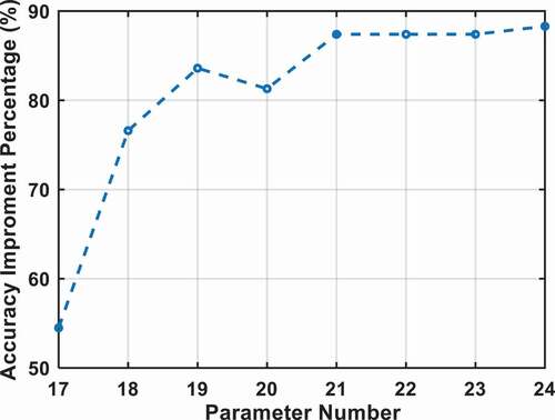
The table indicated the SISRE of all schemes are smaller than 10 cm for the JASON-2 satellite and the fitting precision can be improved by introducing new parameters. However, the figure also indicates that fitting accuracy is not always reduced as the parameter number increases. Introducing the radial range rate $\dot{r}$ contributes to about 54.5% precision improvement. A more substantial improvement can be achieved by introducing two harmonic terms $C_{us3}$ and $C_{uc3}$, which achieved 76.6% precision improvement subject to the GPS LNAV. The 21 parameter scheme achieves the SISRE of the fitted orbit of about 1.1 cm, and introducing more parameters does not bring obvious precision improvement. Hence, it is not necessary to introduce more parameters into the ephemeris set. The optimal 21 parameter set captured the first and the tertiary peaks of $r$ and $u$ in their spectrum, which also confirmed the reasonability of the selected parameter set. Table 4 also indicates the most optimal parameter set includes both the linear trend terms and new harmonic terms, while good fitting accuracy is achievable with only a few additional parameters, rather than all 14 extended parameters. Within the three directions, the cross-track always achieves the best precision and the along-track achieves slightly poorer accuracy than the other two directions. In most cases, the ephemeris fitting achieves convergence within four iterations. However, when the design matrix is ill-posed, it takes more iterations or even divergence.

4.3. Ill-posed problem in ephemeris fitting

The ill-posed problem is a really annoying issue in the fitting procedure, so introducing new parameters needs to be very careful to avoid this problem. Sometimes, the introduced parameters are strongly correlated to existing parameters, which leads to fitting accuracy degradation or iteration divergence. The ill-posed problem can be diagnosed by examining the condition number of the normal equation, given as(Xu 2003):

(16) $\mathrm{C}\mathrm{o}\mathrm{n}\mathrm{d}=\frac{{\lambda }_{\mathrm{m}\mathrm{a}\mathrm{x}}}{{\lambda }_{\mathrm{m}\mathrm{i}\mathrm{n}}}$(16)

where ${\lambda }_{\mathrm{m}\mathrm{a}\mathrm{x}}$ and ${\lambda }_{\mathrm{m}\mathrm{i}\mathrm{n}}$ are the maximum and minimum eigenvalue of the matrix to be examined.

In the ephemeris fitting problem, many parameter combinations are excluded since they are numerically unstable. Table 5 gives some examples to demonstrate the impact of the ill-pose condition on the orbit fitting. The 20-parameter scheme SISRE is larger than the 19-parameter one, which is because $\dot{u}$ is strongly correlated to other elements, which results in a larger design matrix condition number and thus estimated parameters less accurate. For these ephemeris designs with more than 24 parameters, the condition number becomes unacceptable for many combinations, which may lead to the orbit fitting failure. This is also one of the reasons that we attempt to avoid introducing too many parameters in the orbit fitting procedure.

Table 5. Comparison of the condition number and fitting accuracy for different parameter sets

Scheme	Condition number	Accuracy/m
19 parameters	4.08e+09	0.011
20 parameters	5.08e+14	0.013
21 parameters	8.36e+06	0.008

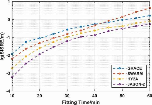
4.4. Impact of fitting interval on the fitting accuracy

The fitting interval is an important parameter for the broadcast ephemeris. GNSS usually employs 1 - 2 hours fitting interval to keep the broadcast ephemeris accurate. The LEO satellites have more complicated dynamics and shorter orbit periods, so the fitting window length is much smaller than the GNSS satellites. To identify the optimal fitting interval, we tested the four satellites with their fitting intervals varying from 10 to 60 min. The optimal 21-parameter set identified previously was adopted in this study and the SISRE accuracy is presented in Figure 5. The figure indicates the fitting error are strongly affected by both orbit height and the fitting interval. Generally, satellite with higher orbit height achieves better fitting accuracy and a smaller fitting interval means better fitting accuracy. A 10-min fitting interval achieves centimeter-level fitting accuracy, while a 55-min fitting interval only achieves several decimeters or even over 1-meter fitting accuracy. Assuming the acceptable fitting SISRE criterion is 10 cm, the feasible fitting interval varies between 20 to 35 min.

Figure 5. LEO satellite orbit fitting residuals at different orbit altitudes.

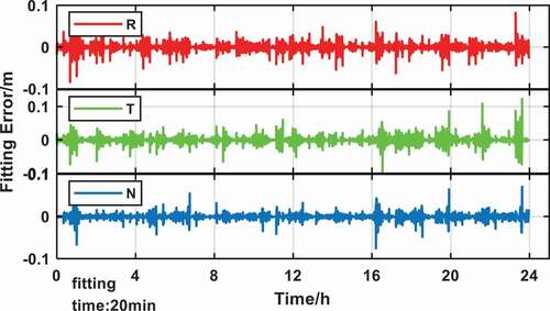
The fitting error time series for JASON-2 Satellite is presented in Figure 6. It reveals that the fitting error may be slightly different over time, but the fitting residuals keep smaller than a few centimeters. There are no systematical biases in the fitting errors, so the fitted orbit can describe the dynamics of the LEO orbit well.

Figure 6. Time series of JASON-2 satellite fitting error for 24 hours using a 20 min fitting window length.

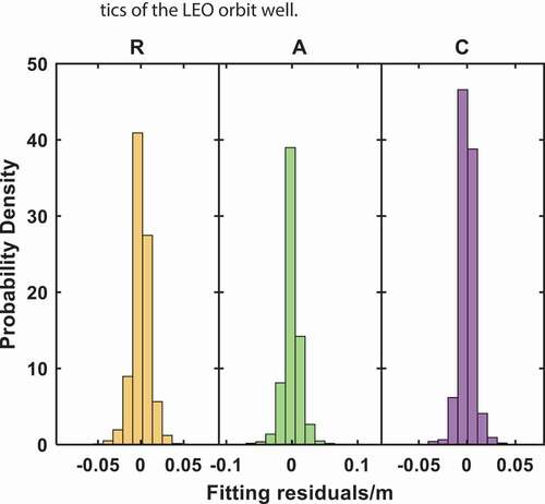
The distribution of the fitting residuals over 20 min period was evaluated and the results are presented in Figure 7. The mean values of the fitting residuals are 7 mm, 8 mm and 5 mm in the radial, along-track, and cross-track respectively. The standard deviations of the fitting residuals are less than 1.3 cm for all three directions. Hence, the 21-parameter broadcast ephemeris can describe the characteristics of the LEO orbit well.

Figure 7. Fitting residuals distribution of JASON-2 satellite for 24 h using a 20 min fitting window length.

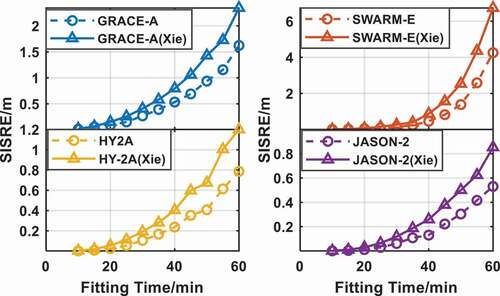
The fitting accuracy of the proposed parameter set can also be validated with external models. For example, Xie et al. (2018) analyzed the LEO ephemeris fitting problem and recommended a 20-parameter set. We compared our method with Xie’s model and the results are presented in Figure 8. Xie recommended introducing four extra parameter to the 16-parmeter set, given as ($C_{rs3},C_{rc3},\dot{a},\dot{n}$), while our model is a 21-parameter set. The comparing results indicate that our 21-parameter achieves a better ephemeris fitting accuracy for all four satellites and the fitting accuracy is improved by 30% on average.

Figure 8. Ephemeris fitting accuracy comparison between 21-parameter model and Xie’s 20-parameter model.

5. Accuracy evaluation of the predicted LEO ephemeris

5.1. The procedure of real-time ephemeris generation

In practice, the broadcast ephemeris needs to be generated with the predicted orbit to support the real-time navigation applications. Hence, the real-time ephemeris contains both the orbit prediction error and the orbit fitting error, while existing research only focused on analyzing the orbit fitting error, which may lead to an over-optimistic expectation of the LEO broadcast ephemeris accuracy. In order to investigate the performance of the real-time LEO broadcast ephemeris, we further tested the orbit fitting precision based on the predicted orbit.

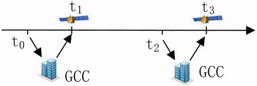
In this study, we assume the broadcast ephemeris was generated at the Ground Control Center (GCC). The procedure of the real-time LEO broadcast ephemeris generation can be illustrated in Figure 9. The onboard GNSS observations are downloaded to the ground and the predicted LEO broadcast ephemeris messages are uploaded periodically and the period is illustrated as t₁ - t₃ in this figure. At the t0 epoch, all the onboard GNSS observations before the t₀ epoch are successfully downloaded to the ground center and the ground center started LEO precise orbit determination and prediction. Then the LEO broadcast ephemeris was fitted based on the predicted orbit and then uploaded to the LEO satellite at t₁ and the LEO satellite starts broadcasting the updated ephemeris. The updated ephemeris is valid until the next period starts, which is marked as t₃ in the figure. However, before starting a new period, the onboard GNSS data until t₂ should be successfully collected and the new ephemeris should be generated and uploaded to the LEO satellite. In this workflow, the LEO prediction period is t₀ to t₃, while the valid ephemeris period is t₁ to t₃.

Figure 9. Flowchart of the real-time LEO broadcast ephemeris generation.

Based on the LEO precise orbit determination results, a short-term prediction of the LEO orbit can maintain centimeter-level accuracy(see Figure 10). With the given initial position and velocity, the LEO orbit can be propagated with high precision force numerical integration. The prediction accuracy depends on the underlying force models. In this study, the dynamic models used in LEO orbit prediction are listed in Table 6. Then the orbit parameters are fitted to generate the real-time LEO broadcast ephemeris based on the predicted orbit.

Figure 10. SWARM-E satellite prediction residuals for 50 min prediction.

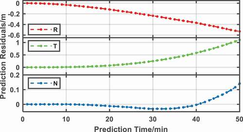
Table 6. Force model used in the LEO orbit prediction

Parameters	Configurations
Gravity Model	GGM03S 120*120 (Tapley et al. 2007)
Solid Tide	IERS 2010 (Petit and Luzum 2010)
Ocean Tide:	IERS 2010 (Petit and Luzum 2010)
Planetary	Mercury, Venus, Mars, Jupiter, etc.
Solar Radiation	Cannon Ball (Fliegel, Gallini, and Swift 1992)
Atmosphere Density Model	NRLmSISE00 Model (Picone et al. 2002; Montenbruck, Steigenberger, and Hauschild 2015)
Relativity	Applied
Integrator	Runge-Kutta with variable order

5.2. LEO predicted ephemeris accuracy evaluation

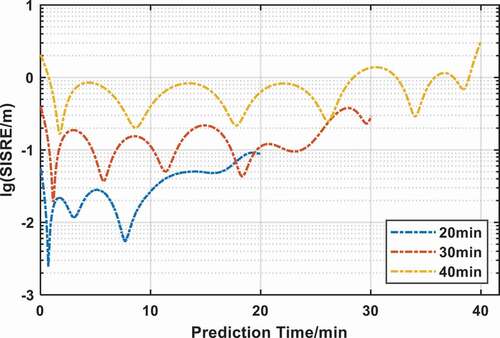
The three LEO satellites, SWARM-E, HY-2A and JASON-2 are used to evaluate the accuracy of the predicted LEO ephemeris. The SISRE of the SWARM-E satellite ephemeris error over 20-min, 30-min, and 40-min prediction are presented in Figure 11. The 21-parameter scheme was used to fit the predicted orbit. The figure shows that the longer period leads to a larger overall SISRE. The SISRE is less than 10 cm for the 20-min prediction. The SISRE increases to better than 20 cm for 30 min prediction and the 40-min prediction scheme achieves a sub-meter level accuracy. Given the 10-centimeter SISRE criterion, the feasible prediction period is less than 20 min.

Figure 11. Predicted ephemeris accuracy variation of SWARM-E satellite with a different prediction time.

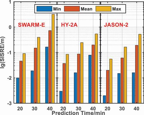
We tested the SISRE of the predicted ephemeris with the LEO satellite from different orbit heights and the results are presented in Figure 12. The figure shows that the SISRE is also affected by the orbit height. The mean SISRE for the JASON-2 satellite is only 2 cm for 20 min prediction, while the error increases to 19 cm for 40 min prediction. Both HY-2A and JASON-2 satellites can keep prediction SISRE smaller than 10 cm for 30 min, while the SWARM-E satellite can maintain 10 cm prediction SISRE for less than 20 min. Higher orbit is beneficial for maintaining the LEO broadcast ephemeris accuracy.

Figure 12. Comparison of SISRE for different satellites under different prediction periods.

6. Conclusions

The design of the precise broadcast ephemeris is an indispensable issue to support LEO augmented real-time precise positioning applications. The LEO satellite suffers more complicated dynamic conditions, while the LEO-NA applications require higher broadcast ephemeris precision. In this study, the characteristics of the LEO orbit are analyzed to identify the additional parameter candidates to the extended ephemeris set. Multiple feasible schemes with different parameter numbers were tested and the optimal parameter set in each parameter number group was identified. The global optimal LEO broadcast ephemeris set was then identified by trading-off between the orbit fitting accuracy and the parameter number. A 21-parameter set was proposed for LEO broadcast ephemeris, which achieves 87.3% fitting accuracy improvement subject to the GPS LNAV scheme. The fitting error characteristics and the optimal fitting window length were also examined and the results based on four in-orbit satellites indicate that 20 - 50 min fitting interval can meet 10 cm SISRE criteria. This paper also considered the generation of LEO broadcast ephemeris in real-time and thus the orbit prediction error was also considered to avoid over-optimistic evaluation of the real-time LEO broadcast ephemeris. The results indicate that the precision of the fitted broadcast ephemeris with the predicted orbit is related to the orbit height. For the LEO with a higher than 500 km orbit, it is possible to achieve better than 10 cm SISRE with 20 min orbit prediction.

Disclosure statement

No potential conflict of interest was reported by the author(s).

Data availability statement

All the LEO orbit data used in this study are publicly accessible. The data can be downloaded at following addresses. GRACE-A:https://earth.esa.int/; SWARM-E:https://swarm-diss.eo.esa.int; HY-2A:https://cddis.nasa.gov/; JASON-2:https://urs.earthdata.nasa.gov/

Additional information

Funding

This study was supported by the National Natural Science Foundation of China [grant number 42074036] and the Fundamental Research Funds for the Central Universities.

Notes on contributors

Xueli Guo

Xueli Guo is a postgraduate student at Wuhan University. His main research interests are GNSS data processing and LEO orbit determination.

Lei Wang

Lei Wang is an associate research fellow in the State Key Laboratory of Information Engineering in Surveying, Mapping and Remote Sensing, Wuhan University. He received a Ph.D. degree in Electronical Engineer and Computer Science from the Queensland University of Technology, Australia in 2015. His research interest includes LEO navigation augmentation, GNSS precise positioning and LEO orbit determination

Wenju Fu

Wenju Fu is a Postdoc researcher, His research interest includes GNSS data processing and LEO orbit determination

Yingbo Suo

Yingbo Suo is a Ph.D. student, his research interest including GNSS/INS integration and LEO orbit determination

Ruizhi Chen

Ruizhi Chen is a professor of State Key Laboratory of Surveying, Mapping and Remote Sensing Information Engineering, Wuhan University, and director of the laboratory. His main research interests include smart-phone ubiquitous positioning and satellite navigation and positioning.

Hongxing Sun

Hongxing Sun is an associate Professor of State Key Laboratory of Surveying, Mapping and Remote Sensing Information Engineering, Wuhan University, his research interest includes GNSS/INS integration.

References

- Chen, L., W. Jiao, X. Huang, C. Geng, L. Ai, L. Lu, and Z. Hu. 2013. “Study on Signal-In-Space Errors Calculation Method and Statistical Characterization of BeiDou Navigation Satellite System.” Paper presented at the China Satellite Navigation Conference (CSNC), Berlin, Heidelberg.
- Chen, R., L. Wang, D. Li, L. Chen, and W. Fu. 2019. “A Survey on the Fusion of the Navigation and the Remote Sensing Techniques.” Acta Geodaetica et Cartographica Sinica 48 (12): 1507–1522. doi:https://doi.org/10.11947/j.AGCS.2019.20190446.
- Choi, J.H., G. Kim, D.W. Lim, and C. Park. 2020. “Study on Optimal Broadcast Ephemeris Parameters for GEO/IGSO Navigation Satellites.” Sensors 20 (22): 6544. doi:https://doi.org/10.3390/s20226544.
- Dong, X., C. Hu, T. Long, and Y. Li. 2016. “Numerical Analysis of Orbital Perturbation Effects on Inclined Geosynchronous SAR.” Sensors 16 (9): 1420. doi:https://doi.org/10.3390/s16091420.
- Du, L., Z. Zhang, J. Zhang, L. Liu, R. Guo, and F. He. 2015. “An 18-element GEO Broadcast Ephemeris Based on Non-Singular Elements.” GPS Solutions 19 (1): 49–59. doi:https://doi.org/10.1007/s10291-014-0364-x.
- Fang, S. 2017. “Model Design of Broadcast Ephemerides for LEO Augmentation Navigation Satellites.” Master, Information Engineering University.
- Fang, S., L. Du, Y. Gao, P. Zhou, and Z. Liu. 2019. “Orbital Elements Ephemerides and Interfaces Design of LEO Satellites.” Acta Geodaetica et Cartographica Sinica 48 (2): 198–206. doi:https://doi.org/10.11947/j.AGCS.2019.20170701.
- Fliegel, H.F., T.E. Gallini, and E.R. Swift. 1992. “Global Positioning System Radiation Force Model for Geodetic Applications.” Journal of Geophysical Research-Solid Earth 97 (B1): 559–568. doi:https://doi.org/10.1029/91jb02564.
- Fu, X., and M. Wu. 2012. “Optimal Design of Broadcast Ephemeris Parameters for A Navigation Satellite System.” GPS Solutions 16 (4): 439–448. doi:https://doi.org/10.1007/s10291-011-0243-7.
- Ge, H.B., B.F. Li, S. Jia, L.W. Nie, T.H. Wu, Z. Yang, J.Z. Shang, Y.N. Zheng, and M.R. Ge. 2021. “LEO Enhanced Global Navigation Satellite System (Legnss): Progress, Opportunities, and Challenges.” Geo-spatial Information Science 1–13. doi:https://doi.org/10.1080/10095020.2021.1978277.
- Huang, H. 2012. “Research on the Broadcast Ephemeris Parameters Model and Its Fitting Algorithm.” Master, Nanjing University.
- Li, X., X. Li, F. Ma, Y. Yuan, K. Zhang, F. Zhou, and X. Zhang. 2019. “Improved PPP Ambiguity Resolution with the Assistance of Multiple LEO Constellations and Signals.” Remote Sensing 17: 408. doi:https://doi.org/10.3390/rs11040408.
- Li, X., K. Jiang, and X. Dong. 2020. “A Navigation Augmentation Method Based on Combining BDS with LEO Constellation and Its Performance Analysis.” Radio Communications Technology 46 (2): 234–238.
- Li, X., F. Ma, X. Li, H. Lv, L. Bian, Z. Jiang, and X. Zhang. 2018. “LEO Constellation-augmented multi-GNSS for Rapid PPP Convergence.” Journal of Geodesy 93 (1): 749–764. doi:https://doi.org/10.1007/s00190-018-1195-2.
- Meng, L., J. Chen, J. Wang, and Y. Zhang. 2021. “A Broadcast Ephemeris Design of LEO Navigation Augmentation Satellites Based on the Integration-Type Ephemeris Model.” Measurement Science and Technology 32 (8): 085009. doi:https://doi.org/10.1088/1361-6501/abfaf5.
- Misra, P., and P. Enge. 2006. Global Positioning System: Signals, Measurements and Performance. 2nd ed. Lincoln, MA: Ganga-Jamuna Press.
- Montenbruck, O., P. Steigenberger, and A. Hauschild. 2015. “Broadcast Versus Precise Ephemerides: A Multi-GNSS Perspective.” GPS Solutions 19 (2): 321–333. doi:https://doi.org/10.1007/s10291-014-0390-8.
- Parkinson, B.W. 2014. “Assured PNT for Our Future: PTA Actions Necessary to Reduce Vulnerability and Ensure Availability.” GPS World 14 (9): 1–10.
- Petit, G., and B. Luzum. 2010. “IERS Conventions (2010).” Bureau International des Poids et mesures sevres (France).
- Picone, J.M., A.E. Hedin, D.P. Drob, and A.C. Aikin. 2002. “NRLMSISE-00 Empirical Model of the Atmosphere: Statistical Comparisons and Scientific Issues.” Journal of Geophysical Research: Space Physics 107 (A12): SIA 15-1-SIA −6. doi:https://doi.org/10.1029/2002ja009430.
- Reid, T.G.R., B. Chan, A. Goel, K. Gunning, B. Manning, J. Martin, A.M. Neish, A. Perkins, and P. Tarantino. 2020. “Satellite Navigation for the Age of Autonomy.” Paper presented at the 2020 IEEE/ION Position, Location and Navigation Symposium, Coronado, CA.
- Remondi, B.W. 2004. “Computing Satellite Velocity Using The Broadcast Ephemeris.” GPS Solutions 8 (3): 181–183. doi:https://doi.org/10.1007/s10291-004-0094-6.
- Sun, H., L. Li, X. Ding, and B. Guo. 2016. “The Precise Multimode GNSS Positioning for UAV and Its Application in Large Scale Photogrammetry.” Geo-spatial Information Science 19 (3): 188–194. doi:https://doi.org/10.1080/10095020.2016.1234705.
- Tapley, B., J. Ries, S. Bettadpur, D. Chambers, M. Cheng, F. Condi, and S. Poole. 2007. “The GGM03 Mean Earth Gravity Model from GRACE.” Paper presented at the AGU Fall Meeting Abstracts, San Francisco.
- Tian, Y., L.X. Zhang, and L. Bian. 2019. “Design of LEO Satellites Augmented Constellation for Navigation.” Chinese Space Science and Technology 39 (6): 55–61. doi:https://doi.org/10.16708/j.cnki.1000-758X.2019.0050.
- Wang, K., and A. El-Mowafy. 2021. “LEO Satellite Clock Analysis and Prediction for Positioning Applications.” Geo-spatial Information Science 1–20. doi:https://doi.org/10.1080/10095020.2021.1917310.
- Wang, L. 2014. “Beidou Satellite Broadcast Ephemeris and Almanac Parameters Fitting Algorithms.” Master, Chang’an University.
- Wang, L., R. Chen, D. Li, G. Zhang, X. Shen, B. Yu, C. Wu, et al. 2018. “Initial Assessment of the LEO Based Navigation Signal Augmentation System from Luojia-1A Satellite.” Sensors (Basel, Switzerland) 18 (11). doi:https://doi.org/10.3390/s18113919.
- Wang, L., R. Chen, B. Xu, X. Zhang, T. Li, and C. Wu. 2019. “The Challenges of LEO Based Navigation Augmentation System – Lessons Learned from Luojia-1A Satellite.” Paper presented at the China Satellite Navigation Conference (CSNC) 2019 Proceedings, Singapore.
- Wang, L., L. Deren, C. Ruizhi, F. Wenju, S. Xin, and J. Hao. 2020a. “Low Earth Orbiter (LEO) Navigation Augmentation: Opportunities and Challenges.” Strategic Study of Chinese Academy of Engineering 22 (2): 144–152. doi:https://doi.org/10.15302/j-sscae-2020.02.018.
- Wang, L., B. Xu, W. Fu, R. Chen, T. Li, Y. Han, and H. Zhou. 2020b. “Centimeter-Level Precise Orbit Determination for the Luojia-1A Satellite Using BeiDou Observations.” Remote Sensing 12 (12): 2063. doi:https://doi.org/10.3390/rs12122063.
- Xiao, Q. 2013. “The Performance Study of Broadcast Ephemeris Parameters and Fitting Method.” Master, Central South University.
- Xiao, Q., X. Cui, X. Jia, Y. Song, and K. Du. 2014. “Performance Comparison of GPS Broadcast Ephemeris Parameters and Their Fitting Algorithms.” Journal of Geodesy and Geodynamics 34 (1): 92–5+9.
- Xiao, Q., X. Cui, Z. Zhou, Z. Nie, C. Huang, and L. Hu. 2016. “Analysis on Broadcast Ephemeris Parameters and Fitting Algorithms of GLONASS and GPS.” Journal of Navigation and Positioning 4 (3): 20–25. doi:https://doi.org/10.16547/j.cnki.10-1096.20160305.
- Xie, X., T. Geng, Q. Zhao, X. Liu, Q. Zhang, and J. Liu. 2018. “Design and Validation of Broadcast Ephemeris for Low Earth Orbit Satellites.” GPS Solutions 22 (2). doi:https://doi.org/10.1007/s10291-018-0719-9.
- Xu, P. 2003. Random Simulation and GPS Decorrelation. Berlin, Heidelberg: Springer.
- Yang, Y. 2016. “Concepts of Comprehensive PNT and Related Key Technologies.” Acta Geodaetica et Cartographica Sinica 45 (5): 505–510. doi:https://doi.org/10.11947/j.AGCS.2016.20160127.