The effects of factor generalization scales on the reproduction of dynamic urban growth

ABSTRACT

The production and selection of driving factors are essential to building a strong Cellular Automata (CA) model of dynamic urban growth simulation. A critical issue that should be addressed is how the spatial representation and the generalization scale of driving factors affect the CA modeling and the simulation results. It is challenging to evaluate the effectiveness of the selected driving factors because they have no true values. To explore the impacts of the generalization scales, we produced nine sets of driving factors at nine scales to calibrate the CA models based on the Particle Swarm Optimization (CA_PSO) and applied them to simulate urban growth of Suzhou during 2000–2020. Our results show that the driving factors at a smaller scale have much better performance in explaining urban growth simulations as inferred by the Explained Residual Deviance (ERD) of the Generalized Additive Models (GAMs). Specifically, the ERD declined from 51.9% to 45.9% as the factor scale became larger during 2000–2020, but there was a peak value (52.2%) at Scale-2. For all simulations during 2000–2020, the CA_PSO models with larger-scale factors have slightly lower overall accuracy and Figure-of-Merit (FOM), which respectively decreased by 3.1% and 4.4% as compared to the CA models with scale-free factors. We concluded that the driving factors at a smaller scale (200 ~ 400 m for point-like facilities and 7 ~ 14 m for line-like facilities) can build more accurate CA models to simulate urban growth patterns, and the optimal scale for factors can be identified using the ERD. This study contributes to the methods of evaluating the effectiveness of driving factor production and reveals the impacts of spatial representation of factors on the CA modeling and simulation considering the factor generalization scales.

KEYWORDS:

• Cellular automata
• urban growth
• driving factors
• scale effects
• generalized additive model

1. Introduction

Urban growth is a complex dynamic process resulting from the comprehensive action of multiple driving factors (Liu et al. 2019; Shao et al. 2020). To reproduce and project urban growth, dynamic modeling is needed to quantify the spatial and temporal patterns of urbanization. Among various simulation models, Cellular Automata (CA) has shown a great capacity for reproducing the main characteristics of dynamic urban growth (Benenson and Torrens 2006; Barreira González, Aguilera-Benavente, and Gómez-Delgado 2015; Cao et al. 2019). In the modeling process, driving factors play an important role that worked as parameters to establish transition rules for CA models (Barreira González, Aguilera-Benavente, and Gómez-Delgado 2015). The driving factors can be divided into the following categories: socioeconomic factors, physical factors, proximity factors, neighborhood factors, and urban planning (Li, Sun, and Fang 2018). For dynamic urban growth and land-use change modeling using CA models, the essential issues of driving factors usually include their data source, identification, selection, scale definition, representation, visualization, and evaluation (Wang et al. 2011; Wu et al. 2012). A few of these issues including factor identification and selection are well addressed in the literature (Wang et al. 2011; Li, Zhao, and Xu 2017; You and Yang 2017; Kantakumar, Kumar, and Schneider 2020). However, the impact of factor representation and its scale definition on the CA modeling is a research gap in the literature because there are no true values for the factors (Wu et al. 2012; Tong and Feng 2019). Further studies on the representation and evaluation of driving factors are necessary for building a more accurate model for urban growth.

Many methods such as Logistic Regression (LR), Survival Analysis (SA), Relative Importance Analysis (RIA), to name a few, have been applied to identify the determinants of urban growth and quantify the spatiotemporally varying effects of driving factors (Chen et al. 2016; Shahbazian et al. 2019; Kantakumar, Kumar, and Schneider 2020). The factors driving urban growth are numerous and often highly correlated (Ku 2016), causing the variable multicollinearity then reducing the simulation accuracy. For example, the RIA-based feature selection method (Kantakumar, Kumar, and Schneider 2020) can measure the contribution of each variable to urban growth to avoid variable multicollinearity. The factors explaining dynamic urban growth also manifest spatiotemporal heterogeneity (Shafizadeh-Moghadam and Helbich 2015; Li, Sun, and Fang 2018; Qian et al. 2020; Xing et al. 2020). The methods of factor selection can be roughly divided into two categories: empirical-statistical methods and data-mining techniques. The commonly used empirical-statistical models include logistic regression (Shu et al. 2014; Salem, Tsurusaki, and Divigalpitiya 2019), Geographically Weighted Regression (GWR) (Shafizadeh-Moghadam and Helbich 2015; Li, Zhao, and Xu 2017), structural equation modeling (Eboli, Forciniti, and Mazzulla 2012), and analytic hierarchy process (Osman, Divigalpitiya, and Arima 2016). Although the empirical-statistical methods are robust and easy to understand, they are weak in handling multimodal data and nonlinear relationships (Müller, Leito, and Sikor 2013; You and Yang 2017). The data-mining techniques have great potential to explore the complex relationship between driving factors and urban growth. Wang et al. (2011) showed that the factors selected by the rough data set theory can better explain urban expansion than the original factors while reducing the number of factors. You and Yang (2017) found that the random forest regression is suitable for identifying the determinants of urban expansion because this method can consider the marginal effect of each independent variable. These studies provided modelers with reliable strategies for identifying and selecting appropriate factors to build an accurate urban growth model. However, before the factor selection, the factor representation should be conducted, and this has not been well addressed in the literature. For example, a proximity factor is usually produced using the distance of each cell to the urban infrastructure such as hospitals, schools, banks, and railway stations, which are considered typically spatial point or line features in Geographical Information Systems (GIS). These facilities are usually generalized as points or lines with no scales, which can only represent the location of these features. GIS-based points or lines (facilities) with different scales should lead to different driving factors. These imply that the generalization scale (here refers to the scale that shows different details of the spatial entities) substantially affects the representation of driving factors, then the simulation results.

In addition, the effectiveness of the representation of each factor needs to be examined quantitively. CA models can be evaluated in three aspects: the input dataset, the modeling procedure, and the simulation results (Tong and Feng 2019). Great efforts have been made to evaluate the procedure and the results of the CA models (Vliet, Bregt, and Hagen-Zanker 2011; Barreira González and Barros 2017; Pinto, Antunes, and Roca 2017; Wu et al. 2019). However, the evaluation of the input datasets as the initial source of model uncertainty has not received enough attention (Yeh and Li 2006; Tayyebi, Tayyebi, and Khanna 2014). Among few works concerning the input datasets, for example, Wu et al. (2012) analyzed the neighborhood configuration considering its capacity of resisting disturbance from data source errors. In contrast, the effectiveness and evaluation of driving factors have not been addressed in the literature, which mostly is attributed to the fact that there are no true values for the factors. Driving factor maps are important components of the model inputs, and their evaluation is of great significance to building accurate models. However, since there are no true values for most of the urban growth driving factors (Tong and Feng 2019), their evaluation has always been a difficult issue that has not been discussed in the literature.

Our study is aimed at solving the following two questions: 1) How does the spatial representation of driving factors affect the simulation results of urban growth patterns? 2) Can we properly evaluate the driving factors without their true values? To answer the former question, we planned to design a multi-scale spatial representation scheme and compare the changes in the simulation results with the factors at different scales. The key to the multi-scale representation is the generalization of geographical information (Yang et al. 2009). Among various types of driving factors, the distance variables are usually used to represent the promotive effects on urban growth, where a site with better accessibility to major transport networks or facilities is more likely to transform to an urban state (Lawal and Anyiam 2019). Therefore, this study is aimed to express and evaluate the proximity factors and their roles in the CA modeling of urban growth. Specifically, the point-like facilities (e.g. hospitals) have their influence ranges as defined by the radius; the line-like facilities (e.g. roads) have their influence ranges as defined by the width, where the radius indicates the half-width of the lines. These different radii should have substantial effects on the urban growth modeling.

The evaluation of driving factors can be indirectly conducted using Generalized Additive Models (GAMs). The GAM uses a smoothing function to build nonlinear relationships between the dependent variables and the independent variables, and the output of the model can simply reflect the effects of the predictive variables (Larsen 2015). The model has been successfully used to reveal the complex relationships between urban growth and its driving factors (Pravitasari et al. 2015). It can also be used to quantify the contribution of each factor of urban growth by using the Explained Residual Deviance (ERD) of the model (Wood 2006). Therefore, this model should be useful to evaluate the impacts of factors on the urban growth modeling, then compare different factors to evaluate them indirectly.

With a case study, we proposed an evaluation scheme of multi-scale factor representation and examine the impacts of the scale on the factors and the modeling results. In this study, we tested our evaluation method using the CA model (CA_PSO) based on the Particle Swarm Optimization (PSO), and took Suzhou city as the case study area. The urban growth simulation model was calibrated with a set of driving factors at multiple generalization scales. We compared the simulation results with different scales of driving factors as the input to explore the impacts of generalization scales on the urban growth modeling. We constructed GAMs to capture the changes in the explanatory ability of each factor to urban growth using the ERD. Since driving factors are key inputs of an urban growth model, our study should help to optimize the simulation models and result in better simulation results.

2. Methodology

2.1. Study area and the multi-scale dataset

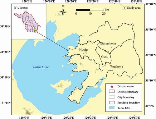
Suzhou is a metropolis located in the southeast of Jiangsu Province and is about an hour’s drive from Shanghai (Figure 1(a)). It is a major economic center of Jiangsu and an important hub of the Yangtze River Delta urban agglomeration. The city is situated on the lower reaches of the Yangtze River and the shores of the Taihu Lake. Suzhou is a fast-growing urbanizing area city in China because of its excellent geographical location and economic development. In 2019, its Gross Domestic Product (GDP) was about 1923 billion Chinese yuan, ranking among the top six in Chinese mainland. With the rapid economic development, urbanization in Suzhou is also accelerating. According to the Suzhou local government, the urbanization rate of Suzhou city reached 76% in 2018. A comparison of urban land-use patterns in 2000 and 2020 shows that the urban land is spreading around Gusu District at a very fast rate. Our study focuses on the core four districts of Suzhou including Gusu, Xiangcheng, Wuzhong, and Huqiu (Figure 1(b)), which cover an area of 1644 km² with the Taihu Lake excluded.

Figure 1. The study area of Suzhou: (a) the study site in Jiangsu and (b) the four districts of study area Suzhou.

For building the CA_PSO model, we acquired the land-use change as the response variable by classifying the Landsat images in 2000, 2010, and 2020. In this paper, we considered three land-use types including urban, non-urban, and water bodies. We took the socioeconomic factors, physical factors, and proximity factors as the explanatory variables that drive urban growth of Suzhou. Table 1 shows the data sources of the vector and raster data used in this study. We extracted eight proximity driving factors by calculating the Euclidean distance of each cell to the facilities (Figure 2) to represent the spatial accessibility to the infrastructure.

Figure 2. The vector formatted data of the facilities to extract the proximity driving factors.

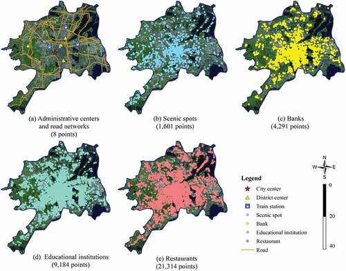
Table 1. The independent variables used to build the CA_PSO models.

Variable	Meaning	Data source
D-city	Euclidean distance to the city center	Administrative map
D-district	Euclidean distance to district centers	Administrative map
D-bank	Euclidean distance to banks	OpenStreetMap
D-station	Euclidean distance to train stations	OpenStreetMap
D-education	Euclidean distance to educational institutions	OpenStreetMap
D-scene	Euclidean distance to scenic spots	OpenStreetMap
D-restaurant	Euclidean distance to restaurants	OpenStreetMap
D-road	Euclidean distance to main roads	OpenStreetMap
GDP	An estimate of GDP derived from satellite data	NOAA National Centers for Environmental Information (NCEI) information
PPP	The estimated number of people per pixel	WorldPop project website
DEM	Terrain conditions	Geospatial data cloud

2.2. The production of multi-scale factors

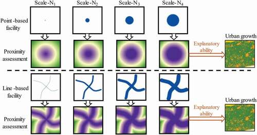
High-credibility driving factors are the prerequisite for deriving accurate CA transition rules. The credibility of factors is not only dependent on the accuracy of the data source but also affected by the factor representation method. The driving factors can be expressed in various methods (Zhang and Su 2016), which emphasize different characteristics of the factor attributes. In our study, we proposed a new method to produce the proximity factors considering their generalization scales. The generalization scale was defined as the radius of the vector features representing the facilities. For point facilities (e.g. banks), the radius indicates the servicing capability; for linear facilities (e.g. roads), the radius indicates the possible width. Figure 3 shows the production of multi-scale proximity factors graphically with a case of point-like facilities and a case of line-like facilities. The point-like facilities can be expressed in two ways: 1) points with no size, and 2) circles with different radii. The line-like facilities can be expressed in two ways: 1) polylines without width, and 2) linear polygons with different widths. Figure 3 shows that different generalization scales lead to different details of the spatial entities, producing different driving factors, then different CA transition rules, CA models, and simulation results. The relationship between the driving factors of multi-scale representation and the simulation results of urban growth can be built, then explained by the explanatory ability of the factors.

Figure 3. An example of the spatial representation of the point and line-like diving factors of different generalization scales.

Table 2 shows that the nine scales that we used to produce the driving factors. The driving factors at Scale-0 are scale-invariant and used as a comparison with the factors at other scales to explore the influences on the simulation results. Except for the Scale-0, the influence radius of the point factor ranges from 200 m to 1600 m, with an interval of 200 m (Table 2). Figure 4 shows a representation of the point factors at different scales, where the selected facility is the banks in this study. The radius of roads was defined according to the Chinese “Code for design of urban road engineering” (CJJ 37–2012-2016), ranging from 7 m to 35 m (Table 2). Compared with the extent of the study area, the radius of the line features among is too small to be distinguished visually. We calculated the Euclidean distance to the facilities at each scale to produce multi-scale driving factors. Figure 5 shows the D-bank factor at nine scales where the densely distributed bank POIs visually overlapped at a very large scale and the details in the distance of each cell to the POIs cannot be well-reflected.

Figure 4. An example of bank factors represented at the 8 different generalization scales except for the Scale-0.

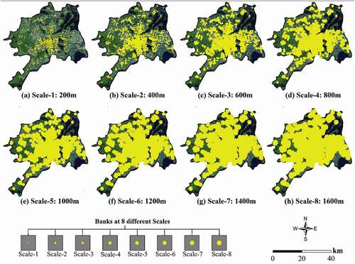
Figure 5. An example of driving factors (D-bank) at the nine generalization scales.

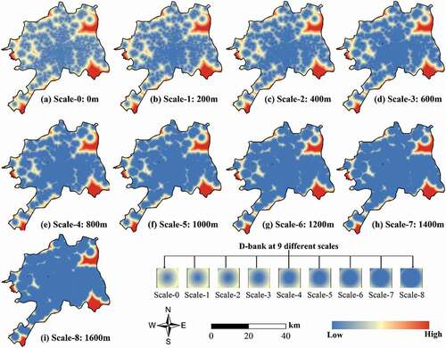
Table 2. The generalization scales used to extract the point and line-like driving factors.

Feature	Scale-0	Scale-1	Scale-2	Scale-3	Scale-4	Scale-5	Scale-6	Scale-7	Scale-8
R-point (m)	0	200	400	600	800	1000	1200	1400	1600
R-line (m)	0	7	11	15	19	23	27	31	35

R-point is the radius of the point features, and R-line denotes half-width of the line features.

2.3. The calibrated CA model (The CA_PSO model)

The CA models are self-organizing,bottom-upapproaches to simulate complex systems using a set of transition rules (He et al.2006). The modeling approach determines the state of cells at the next time as a function (comprehensive impacts) of the state of the cells and their neighborhoods at present according to a set of transition rules (Aburas et al. 2016). The transition function can be given by (White and Engelen 1993):

(1) $Cellstat{e}_{i,t+1}=TransF\left(\begin{array}{c}Cellstat{e}_{i,t},Trans{P}_i,\\ Neig{h}_i,Con{s}_i,Ran{D}_i\end{array}\right)$(1)

where $TransF$ denotes the transition rules; $Cellstat{e}_{i,t+1}$ and $Cellstat{e}_{i,t}$ respectively denote the state of the cell $i$ at the time t and time t + 1; $Trans{P}_i$ denotes the land transition potential calculated with the driving factors; $Neig{h}_i$ denotes the neighborhood effects that indicate the interaction among nearby cells; $Con{s}_i$ denotes both the nonspatial and spatial constraints; and $Ran{D}_i$ denotes a stochastic disturbance. For defining the interaction of nearby cells, we applied a 5 × 5 square neighborhood following earlier publications (Feng et al. 2019).

The land transition potential ($Trans{P}_i$) is calculated from a set of spatial driving variables. The potential can be calculated by (Arsanjani et al. 2013):

(2) $Trans{P}_i\left(w_0,\cdots ,w_n\right)=\frac{\mathrm{e}\mathrm{x}\mathrm{p}\left(w_0+{\sum }_{i=1}^n\left(w_i\times x_i\right)\right)}{1+\mathrm{e}\mathrm{x}\mathrm{p}\left(w_0+{\sum }_{i=1}^n\left(w_i\times x_i\right)\right)}$(2)

where $Trans{P}_i\left(w_0,\cdots ,w_n\right)$ represents the transition potential of the cell $i$; $\left(w_1,\cdots ,w_n\right)$ indicates the weight of each variable $\left(x_1,\cdots ,x_n\right)$ and $w_0$ is a constant. The constant and weights $\left(w_0,\cdots ,w_n\right)$ are the CA parameters, which can be retrieved by different methods such as LR and GWR.

The possible spatial correlation of the variables may lead to low accuracies of simulations. Thus, the parameters that can minimize the modeling residuals are optimal for the urban growth simulation. The modeling residuals (or fitness value) can be given by (Feng et al. 2011):

(3) $\mathrm{m}\mathrm{i}\mathrm{n}F\left(w\right)=\sqrt{\frac{{\sum }_i^N{\left(Trans{P}_i\left(w\right)-Trans{P}_0\right)}^2}{N}}$(3)

where $\mathrm{m}\mathrm{i}\mathrm{n}F\left(w\right)$ is the minimized value of the residuals and can also be considered a fitness function; $w$ represents the CA parameters; $N$ represents the number of sampling cells; $Trans{P}_i\left(w\right)$ is the local transition potential calculated through the LR method; and $Trans{P}_0$ means the actual transition result of the cell.

To solve the fitness function, we applied the PSO method that can produce a better model with much lower residuals (Feng et al. 2018). PSO reflects the global structure of a system through the interactions of the underlying units, where the model’s behavior consistent with the bottom-up approach of CA models. Therefore, the PSO method is very suitable for deriving the transition rules and building CA models, which eliminate the impacts of correlation among driving factors to improve the simulation results. Among many similar optimization algorithms, we chose PSO because it has been widely applied to simulate land-use change and urban growth since it has been proposed by Feng et al. (2011). This study focuses on the representation and evaluation of driving factors, and the PSO-based CA model is appropriate to conduct a useful test.

PSO applies the movement of particle swarms to simulate how birds can cooperate with other nearby birds to find food. The state of a particle in the current time step is associated with its position, velocity and fitness value. The particle in the PSO algorithm can be coded as (Feng et al. 2011)..

(4) $W_i\left(w_{i1},w_{i2},\dots ,w_{in};v_{i1},v_{i2},\dots ,v_{in};F\left(w\right)\right)$(4)

where $w_i$ represents the position of the $i$-th particle, and $v_i$ represents its movement velocity. Each particle in the search space represents a feasible combination of CA parameters (Feng et al. 2011). The search space dimensions correspond to the number of CA parameters.

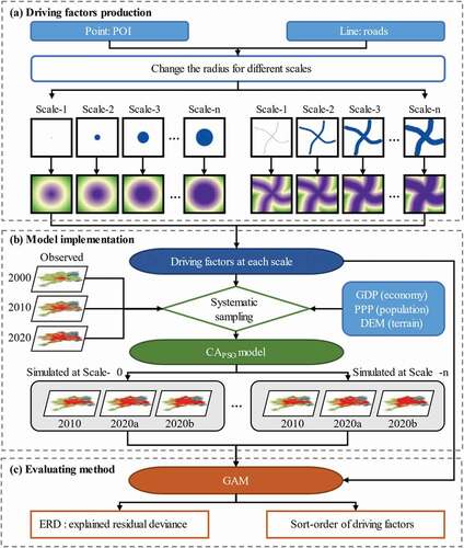
Figure 6 shows the workflow of reproducing the dynamic urban growth with the CA_PSO model for evaluating the effectiveness of driving factors at different scales. The workflow consists of three steps: (1) the production of multi-scale driving factors, (2) the CA_PSO model implementation, and (3) the evaluation of factor effectiveness. We first applied the method in Figure 3 to produce the proximity factors at multiple scales, then produced the land-use maps of three years (2000, 2010, and 2020). Using these datasets, we calibrated the CA_PSO models based on the 2000–2010 urban growth considering the driving factors at nine different scales. We simulated urban growth in 2000–2010, 2000–2020, and 2010–2020, then built GAMs between the simulated urban growth and the driving factors to evaluate their effectiveness at different scales. The evaluation metrics are ERD and the sort-order.

Figure 6. The workflow of the factor effectiveness evaluation with the CA_PSO model. (2020a: 2020 simulated from 2010, and 2020b: 2020 simulated from 2000).

2.4. Evaluation methods to the factor effectiveness

2.4.1. The model accuracy evaluation

The model evaluation directly reflecting the accuracy of the simulation results can be applied to evaluate the effectiveness of driving factors at different generalization scales. Among many methods of model evaluation, the cell-by-cellcomparison is a commonly used approach that can produce several metrics (Pontius 2000). We therefore evaluated the CA_PSO modeling results by comparing them with the actual urban patterns cell by cell. The comparison generates metrics including Hit, Correct rejection, Miss and False alarm. (Pontius et al. 2008). The Hit indicates the actual dynamic urban growth is correctly simulated; the Miss means the actual dynamic urban growth is simulated as non-urban persistence; the False alarm represents actual non-urban persistence is wrongly simulated as dynamic urban growth. We used three metrics to evaluate the simulation results, namely overall accuracy, Figure-of-Merit (FOM) and the Matthews Correlation Coefficient (MCC). The overall accuracy measures the agreement between the simulated and observed land-use maps; FOM indicates the model’s ability to capture urban growth (Pontius et al. 2008); MCC is a metric for the model evaluation when an imbalance exists between the pixels of different classes (Kantakumar, Kumar, and Schneider 2019). They can be given by (Pontius et al.2008; Kantakumar, Kumar, and Schneider 2019):

(5) $Overallaccuracy=\frac{Hit+Correctrejection}{\begin{array}{c}Hit+Correctrejection\\ +Miss+Falsealarm\end{array}}$(5)

(6) $FOM=\frac{Hit}{Hit+Miss+Falsealarm}$(6)

(7) $MCC=\frac{\left(Hit\times Correctrejection\right)-\left(Falsealarm\times Miss\right)}{\sqrt{\begin{array}{c}\left(Hit+Falsealarm\right)\left(Hit+Miss\right)\\ \left(Correctrejections+Falsealarm\right)\\ \left(Correctrejection+Miss\right)\end{array}}}$(7)

2.4.2. The GAM evaluation method

We used the driving factors’ ability to explain the land-use change to examine the effectiveness of the factor production method. The GAM method was applied to quantify the explanatory ability of a driving factor. The GAMs are generalized linear models that allow a flexible relationship between the individual explanatory variables and the dependent variable (Anderson-Cook 2007). Each additive term in the GAM is estimated using a single smoothing function that can explain how the dependent variable changes with the independent variable. The relationship between urban growth and the driving factors in this study is nonlinear, therefore, the model is very suitable for capturing the relationship. Besides, a GAM can accurately describe the contribution of each independent variable to the dependent variable. The GAM can be given by (Feng and Tong 2017)..

(8) $g\left(\mu \right)=a_0+s_1\left(x_1\right)+s_2\left(x_2\right)+s_3\left(x_3\right)+s_4\left(x_4\right)+\dots +s_i\left(x_i\right)$(8)

where $g\left(\mu \right)$ is a function which links the dependent variable and the additive component, $a_0$ denotes the model fitting residuals, and $s_i\left(x_i\right)$ is a smoothing function links the variable $x_i$ to the function $g\left(\mu \right)$.

GAM is a stepwise method that introduces factors one by one based on their ERD. This also reflects that the sort-order of independent variables greatly affects the result of a GAM. A prior factor has a stronger impact on urban growth than a posterior one. The GAM can be applied to quantitatively evaluate the explanatory ability of all factors included by using ERD. The driving factors at a suitable scale can explain more ERD of GAMs. In addition, the sort-order intuitively reflects the relative importance of factors to urban growth (Feng and Tong 2017; Feng et al. 2019; Kantakumar, Kumar, and Schneider 2020).

3. Results

3.1. The scale effects on the model construction

To train our CA_PSO models, we selected 4718 sample points in the study area by using systematic sampling; these were performed using the UrbanCA software (Feng and Tong 2020). The heuristic methods are sensitive to their controlling parameters, the definition of the controlling parameter is critical for constructing the CA_PSO models. We defined the controlling parameters using the default values recommended in UrbanCA. The number of particles was defined as 20 times the sum of the number of variables and an intercept; thus, the particles were 2400 in this study. In addition, the PSO method terminates once it reaches a maximum iteration of 5000 or a fitness tolerance of 1E−10.

We defined the lower and upper bounds of the CA parameters using the LR method for optimizing the CA_PSO models. Table 3 shows the calculated CA parameters by PSO at the nine scales. For the density factors (e.g. GDP and PPP), a positive parameter means a promotive effect on urban growth, and a negative parameter indicates a resistive effect. For distance and surface factors, there is a contrary trend. For example, DEM has negative and high absolute parameters at all nine scales, indicating a greater impetus for urban growth. While the D-city factor has the lowest absolute parameters, indicating its weakest influences. As the scale increased, the effects of D-bank, D-city, and D-district on the dynamic urban growth enhanced but the effects of D-education decreased. The effect of the GDP factor is also reduced in promoting urban development, even changed to be restrained after the Scale-6. The absolute parameter of the D-restaurant increased rapidly as the scale increased to the Scale-6, indicating the high correlation between D-restaurant and urban growth at the Scale-6. However, the restaurants could not play such a decisive role in dynamic urban growth, so this may also indicate that the Scale-6 is not a suitable scale for representing the effects of the restaurants.

Table 3. The calculated CA parameters of the CA_PSO models at the nine different scales.

Variable	Scale-0	Scale-1	Scale-2	Scale-3	Scale-4	Scale-5	Scale-6	Scale-7	Scale-8
Constant	0.953	0.627	0.425	0.329	0.281	0.243	0.215	0.148	0.135
D-bank	−5.535	−5.755	−6.716	−8.613	−11.990	−15.382	−16.555	−24.446	−22.415
D-city	−0.131	−0.111	−0.154	−0.352	−0.530	−0.594	−0.712	−0.926	−1.003
DEM	−51.347	−50.079	−48.490	−47.970	−47.733	−48.742	−49.877	−52.808	−54.481
D-district	0.829	0.817	0.831	0.935	1.002	1.019	1.140	1.381	1.432
D-education	−4.080	−4.230	−5.095	−5.048	−2.590	−1.955	−2.320	−0.941	−0.972
GDP	−0.532	−0.498	−0.437	−0.348	−0.228	−0.109	0.011	0.239	0.341
PPP	−4.398	−4.181	−3.792	−3.571	−3.559	−3.494	−3.471	−3.620	−3.670
D-station	−2.132	−2.088	−2.039	−2.011	−2.046	−2.136	−2.231	−2.145	−2.161
D-restaurant	−6.987	−7.022	−7.754	−9.309	−15.702	−34.684	−3134.62	−5.541	−1.763
D-road	0.662	0.684	0.768	0.767	0.756	0.732	0.652	0.662	0.617
D-scene	2.451	2.302	2.040	1.710	1.363	1.250	1.054	0.517	−0.102

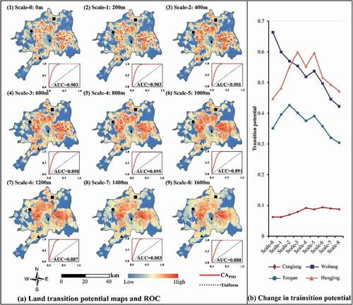
We visualized the land-use transition potential and their Receiver Operating Characteristic (ROC) curves based on the nine sets of driving factors at different scales (Figure 7(a)). All the nine potential maps generally share similar spatial patterns, where high transition potential is mainly observed around the built-up areas. This indicates that the built-up areas exert influences on the surrounding areas. The ROC curve is a useful statistical method to assess the transition potential, with Hit/(Hit + Miss) as the vertical axis and False alarm/(False alarm + Correct rejection) as the vertical axis (Pontius Jr and Si 2014). The Area Under Curve (AUC) measures the reliability of the transition potentials, ranging from 0.5 to 1.0. All the nine transition potential maps have a high AUC (>0.8), which shows that the CA_PSO model is very reliable. As the scale becomes larger, the AUC shows a downward trend, reflecting that the increase in the factor scale will lead to a decrease in the consistency between the estimated and observed transition potential. We compared the transition potential of four spots in four different districts (Canglang street in Gusu, Weitang town in Xiangcheng, Tongan town in Huqiu, and Hengjing Town in Wuzhong) at nine scales (Figure 7(b)). The results show that Canglang, which is closer to the city center, has a lower transition potential and is less affected by the factor scale, while the potential of the other three spots fluctuates greatly with the scale changes. As the scale becomes larger, land with higher urbanization potential is increasingly concentrated around the city center. Since the driving factors at a very large scale cannot reflect the details (Figure 5), the transition potential derived using the large-scale factors also cannot help to allocate the areas with high urbanization potential in the suburbs.

Figure 7. (a) Land transition potential maps and their ROC curves at the nine scales; (b) the change in transition potential of four selected spots.

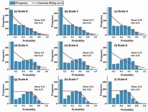
We plotted the land potential distribution to more accurately represent the change in the transition potential (Figure 8). For any scale, the transition potential of most areas is in the range of 0–0.1, showing urbanization potential in most areas is low. The mean potential increases as the scale increases, indicating an increase in the transition potential in the study area. With the scale increases, the Standard Deviation (STD) first becomes larger and reaches its maximum at Scales 4 ~ 6, then decreases after Scale-6. As the factor scale becomes larger, the STD shows that the differences in the transition potential across the study area become larger first and then smaller. The increasing scales lead to a greater potential of urbanization generally, and the potential distribution gradually concentrates toward the median value (0.4–0.6) as the scale increases. We used the Gaussian fitting method to curve-fit the transition potential distribution (red line in Figure 8). The results showed that the potential distribution is closer to the normal distribution when the factor scale becomes large (larger than Scale-5), reflecting that the transition potential distribution with large-scale factors shows stronger randomness. This also indicates that the land transition potential retrieved with large-scale proximity factors is not reliable for building an accurate model.

Figure 8. The distribution of the land transition potential at the nine scales.

3.2. The scale effects on the simulation results

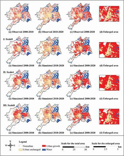
We simulated the land-use patterns of 2010 and 2020 with driving factors at all nine scales (Figure 9). For each scale, there are two simulation results of the land-use pattern in 2020, which are simulated based on the observed land-use patterns in 2010 and 2000, respectively. Figure 9 intuitively shows the observed and simulated land-use change since 2000. Suzhou’s urban growth during 2000–2020 mainly occurred around the Suzhou downtown, and the urban land expanded slowly on the periphery of four districts during 2010–2020. The observed and simulated land-use maps at different scales share similar overall patterns, but the enlarged maps show distinct differences. In comparison, the simulated urban growth pattern is more compact around the built-up areas than the observed pattern. As the scale increased, the non-urban areas surrounding the built-up areas had gradually transformed into the urban state, shaping a larger urban patch around the built-up areas. Suzhou’s urban growth of all three periods shared a similar change trend as the scale of the driving factors became larger. This indicates that the urban cell allocation ability of the CA_PSO model is highly related to the existing built-up areas, which may lead to the failure in capturing urban growth in far suburbs.

Figure 9. The observed and simulated urban growth during 2000–2020 with different driving factors at various scales.

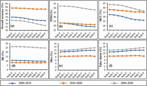
We used six metrics to quantify the simulation accuracies at the nine scales (Figure 10). In all three periods (2000–2010, 2000–2020, and 2010–2020), the overall accuracy, FOM and MCC decreased as the scale increased, suggesting the decreasing modeling performance of the CA_PSO model. Specifically, the performance decrease was caused by the drop in Hit, and the rises in Miss and False alarm with the increasing scale, indicating decreases in both the overall state agreement and change simulation.

Figure 10. The simulation accuracy evaluation at the nine scales of the driving factors.

3.3. The scale effects on the explanatory ability of the driving factors

3.3.1. The scale effects explained by the ERD

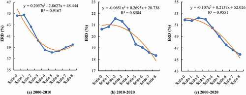
Figure 11 shows that the ERD of GAMs greatly changes with the changing scales. By comparing the results in all three periods, we find that the ERD shows an obvious downward trend generally as the scale increases. We fitted the changing trend of the GAM’s ERD with the changing scale. The ERD’s change curves in all three periods follow quadratic curves. The ERD of 2010–2020 and 2000–2020 showed a similar trend, peaking at the Scale-2 then declining as the scale become larger. The ERD of 2000–2010 reached its peak at Scale-1 and continued to decrease as the scale increased until it reached its lowest value at Scale-5. The ERDs of all three periods reached their peaks at a small scale (< Scale-3), and followed by significant decreases, indicating that the scale with the maximum ERD was the most appropriate for the model construction. The driving factors at such scales have the strongest ability to explain the simulated urban growth. On the contrary, driving factors at a large scale (> Scale-4) cannot well explain urban growth. The explanatory ability of the factors from no scale to the largest scale has dropped by nearly 5%, 3%, and 7% for the three time-periods, respectively. It indicates that the reduction in factor explanatory ability is related to the urban growth rate. The factor explanatory ability decreases faster as the scale becomes larger in a region with a faster urbanization rate.

Figure 11. The ERD of the driving factors for simulating urban growth at the nine scales.

3.3.2. The scale effects explained by the factor sort-order

Table 4 shows the sort-order of each factor at the nine scales, implying the effects of the driving factors on urban growth during 2000–2020. The sort-order changed slightly at small scales (< Scale-3) in the three periods, indicating that minor changes in scale would not cause a significant variation in the factors’ effects on urban growth. However, the sort-order of most factors changed significantly after the Scale-3. Among the factors, D-road showed a relatively low influence on urban growth due to the multicollinearity between D-road and other driving factors. D-bank ranks the first and shows the strongest effects at small scales (< Scale-4), but shows weak effects on urban growth at large scales. In contrast, the effect of GDP on urban growth is significantly increased with the increasing scale, and it ranks the first at large scales (> Scale-6). D-bank, D-education, D-restaurant, and D-scene produced from the densely distributed facilities significantly declined with the increasing scale. In contrast, the D-station, D-district, D-city, and D-road factors produced from sparsely distributed facilities have higher sort-order with the increasing scale. Among the three density-based driving factors, GDP and DEM rank up to the forefront as the scale increases while the sort-order of PPP declines slightly. Among all factors, the scale-invariant factors contributed the most of influences as the scale became larger, implying that the scale increase has led to decreases in the proximity factor’s ability to explain urban growth.

Table 4. The sort-order of driving factors at the nine scales in the three time-periods.

Variable	Scale-0			Scale-1			Scale-2			Scale-3			Scale-4
	2000–2010	2010–2020	2000–2020	2000–2010	2010–2020	2000–2020	2000–2010	2010–2020	2000–2020	2000–2010	2010–2020	2000–2020	2000–2010	2010–2020	2000–2020
D-bank	1	1	1	1	1	1	1	1	1	1	1	1	2	1	1
PPP	2	2	2	2	2	2	2	2	2	3	3	3	4	6	4
D-education	3	3	3	3	3	3	4	3	3	7	7	7	10	10	10
D-station	4	4	5	4	6	5	3	4	5	4	5	5	3	4	5
DEM	5	5	4	5	5	4	5	5	4	5	4	4	5	5	3
D-scene	6	6	7	6	9	8	9	9	9	9	10	10	9	11	11
D-restaurant	7	7	6	7	8	7	8	8	8	10	9	8	8	8	8
D-district	8	8	8	9	7	6	6	6	6	6	6	6	6	3	6
GDP	9	9	9	8	4	9	10	7	7	2	2	2	1	2	2
D-road	10	10	11	10	11	11	7	11	11	8	11	11	7	9	9
D-city	11	11	10	11	10	10	11	10	10	11	8	9	11	7	7
	Scale-5			Scale-6			Scale-7			Scale-8
Variable	2000–2010	2010–2020	2000–2020	2000–2010	2010–2020	2000–2020	2000–2010	2010–2020	2000–2020	2000–2010	2010–2020	2000–2020
D-bank	5	1	1	6	5	3	7	5	5	9	7	6
PPP	3	7	6	4	7	6	2	7	6	4	6	5
D-education	11	11	10	11	10	10	10	10	10	10	10	11
D-station	2	4	4	2	3	4	3	3	3	2	3	3
DEM	4	3	3	3	2	2	4	2	2	3	2	2
D-scene	8	10	11	8	11	11	11	11	11	8	9	9
D-restaurant	9	9	8	9	9	8	9	9	9	11	11	10
D-district	6	5	5	5	4	5	5	4	4	5	4	4
GDP	1	2	2	1	1	1	1	1	1	1	1	1
D-road	7	8	9	7	8	9	6	8	8	6	8	8
D-city	10	6	7	10	6	7	8	6	7	7	5	7

4. Discussion

The effectiveness and credibility of urban growth models are important to their evaluation. However, it is difficult to evaluate the uncertainties in the output of spatial models because there are various possible input data for modeling (Pérez-Molina et al. 2017; Salap-Ayca et al. 2017). As a crucial part of the input of urban growth models, driving factors have many possibilities in category and combination (Zhang and Su 2016). To date, little attention has been paid to the spatial representation and the effectiveness of the driving factors. In our study, we focused on the spatial representation of factors considering the generalization scales, where the size (or the generalization scale) of the facilities is of substantial significance. For example, the scale of a point-like facility means its influencing range or servicing capability that was expressed by the radius; similarly, line-like facilities have their influences at different scales. At nine different scales, we produced nine sets of driving factors that were used to construct nine CA_PSO models to simulate urban growth of Suzhou during 2000–2020. Since the factors have no true values, we proposed a new method to identify the optimal representation of factors by examining their explanatory ability on the simulations.

4.1. The effects of factor scale on the simulations

The generalization scale substantially affects the spatial representation and pattern of driving factors, then affecting the simulation results. The results show that the model performance declined in both end-state and change as the scale of driving factors increased. The transition potential maps indicate that the high transition potential is clustered around the city center as the scale became larger. A visual comparison between Figure 7(a,i) can clearly show the differences. Models of using factors of large-scale failed to capture the dynamic urban growth in far suburbs, leading to a gradual decline in their ability to reproduce past urban growth. This is due to the overlap of the influences of the facilities at the large scales (c.f. Figure 4(g–h)). Specifically, with the increasing scale, the influencing extent of the facilities in densely distributed areas affect each other. Thus, at a large scale of factors, regions with high transition potential would be likely clustered around the built-up areas.

The consequent model evaluation showed more details about the effects of factor scales regarding different periods. The overall accuracies of the three periods are lower than 84%, showing relatively low overall end-state agreement (Figure 10(a)) between the observed and simulated urban patterns by comparing the simulations in the literature (Chudech et al. 2016). Earlier CA publications showed that the overall end-state agreement is closely related to the magnitude of urban growth or urban land-use change throughout the simulation period (Pontius et al. 2008). A higher magnitude (fast urbanization) may lead to lower accuracy while a lower magnitude (low urbanization) may lead to higher accuracy. For this study, the study area Suzhou is a rapidly urbanizing area in east China. The change evaluation that focuses on the areas changing from nonurban state to urban state can well reflect the model performance. Our change evaluation using FOM shows high accuracy (>25%; Figure 10(b)) compared with the literature (Wang, Hou, and Murayama 2018; Feng and Tong 2020), indicating the good performance of the CA_PSO models. The changes in the overall end-state agreement and change evaluation show that, compared to models with scale-free factors, models with greater scales would reduce the modeling accuracy in reproducing urban growth.

4.2. The effectiveness evaluation of factors

The model credibility highly depends on the input driving factors, thus it is critical to evaluate the effectiveness of factors on the modeling results (Wu et al. 2012; Salap-Ayca et al. 2017). We therefore built a bridge between the driving factors and the simulation results using GAM. The explanatory ability of the driving factors was used as the benchmark to evaluate the effectiveness of the factors. The ERD and factor sort-order in GAMs provide quantitative metrics to measure how much can the factors explain the simulations. This explanatory ability can be considered as a metric of the factor effectiveness, which is a comprehensive index for evaluating the input factors in terms of their spatial representation.

In evaluating modeling results, for example, an error matrix needs a comparison between the modeling results and the actual results. However, there are no true values for any driving factor. In addition, the accuracy of the simulation results is affected by several elements, therefore the effectiveness of driving factors cannot be reflected by the model accuracy. Our study indicates that the use of ERD and factor sort-order can provide credible metrics for identifying the optimal factors when there are no true values. Meanwhile, the ERD and sort-order in GAMs are sensitive to the factor scale (i.e. the generalization scale), which helps us to identify the optimal scale that can be used in modeling.

4.3. The optimal representation scheme of factors

Driving factors are approximations of geographic and socio-economic elements, and their visualization may cause the loss of spatial details at various extents (Korporaal, Ruginski, and Fabrikant 2020). Proximity factors are the most important input in modeling dynamic urban growth (Shafizadeh-Moghadam et al. 2017; Mustafa et al. 2018). In this study, we produced the proximity factors from facilities with different spatial details by emphasizing the servicing capabilities. For point-like facilities such as hospitals and shopping centers, it is difficult to define their influencing areas. We therefore examined their servicing distance from 0 km to 2 km. For line-like facilities such as roads and rivers, their real widths can be used to represent the servicing distance. For example, the main roads in Suzhou are about 14 to 70 m in width (i.e. scale), which shows different spatial details in factor maps. To represent different levels of the servicing ability, we utilized driving factors at eight scales in our models (c.f. Table 2).

The ERD and sort-order in GAMs that can evaluate the effectiveness of factors were used to identify the optimal scale of factors. The ERD reached its peak at a small scale (< Scale-3) in each period (c.f. Figure 11), indicating the strongest explanatory ability of the factors at this scale. Because the simulation accuracy and the sort-order changed slightly at a small scale, the scale related to the ERD peak can be considered the most suitable scale for producing factors. We suggest modelers select the optimal scale of factors using the ERD in GAMs before modeling.

5. Conclusions

CA modeling of urban growth is substantially influenced by the production and selection of driving factors. To date, we are not aware of the impacts of the factor representation and generalization scale on the modeling and its outcomes. However, it is very challenging to evaluate the effectiveness of driving factors since there are no true values for them. We produced nine sets of driving factors at nine scales (0 ~ 1600 m for points and 0 ~ 35 m for lines) and used these factors to calibrate the CA_PSO models with a case study of the 2000–2020 urban growth simulation in Suzhou. The relationships between the driving factors and the simulation outcomes were constructed using GAMs. The ERD and sort-order in GAMs were used to quantify the explanatory ability of factors, reflecting their effectiveness in modeling urban growth. Compared with using model accuracy to evaluate the effectiveness of factors, the superiority of GAM is that it can establish a relationship between the factors and the simulation results for quantitative assessment. The results show that the driving factors at a smaller scale have a stronger explanatory ability according to the ERD of the GAM.

This work reveals the influences of factor generalization scales in reproducing urban growth and provides an example of producing driving factors with multiple scales. It provides a new method using the ERD in GAMs to evaluate the effectiveness of driving factors with no true values, where the ERD is very proper to identify the optimal scale for reproducing historical urban growth. The specific scales of factors should be different for different areas, but the scale identification method we proposed in this paper can be widely used in examining urban growth elsewhere. Future work should consider the scale definition of other factors on historical urban growth simulations, and the influence of factor scales on future scenario prediction.

Disclosure statement

No potential conflict of interest was reported by the author(s).

Data availability statement

The datasets and software used in this study are freely available at https://figshare.com/s/1a680869bbbb3b188850.

Additional information

Funding

This work was supported by and the National Natural Science Foundation of China [Grant No. 42071371], and the National Key R&D Program of China [Grant Nos. 2018YFB0505000 and 2018YFB0505400].

Notes on contributors

Yongjiu Feng

Yongjiu Feng received the PhD degree in geomatics from Tongji University, Shanghai, China, in 2009. He is currently a Professor and Associate Dean of the College of Surveying and Geo-Informatics, Tongji University. His research interests include spatial modeling, synthetic aperture radar interferometry, and radar detection of the moon and deep space.

Peiqi Wu

Peiqi Wu is currently working toward the MS degree in geomatics with Tongji University, Shanghai, China. Her research interests include spatial modeling and radar detection of the moon and deep space.

Xiaohua Tong

Xiaohua Tong received the PhD degree in traffic engineering from Tongji University, Shanghai, China, in 1999. He is currently a Professor with the College of Surveying and Geo-Informatics, Tongji University. His research interests include photogrammetry and remote sensing, trust in spatial data, and image processing for high-resolution satellite images.

Pengshuo Li

Pengshuo Li is currently working toward the MS degree in geomatics with Tongji University, Shanghai, China. His research interests include spatial modeling and radar detection of the moon and deep space.

Rong Wang

Rong Wang currently working toward the MS degree in marine sciences with Tongji University, Shanghai, China. Her research interests include spatial modeling and synthetic aperture radar interferometry.

Yilun Zhou

Yilun Zhou is currently working toward the MS degree in geomatics with Tongji University, Shanghai, China. Her research interests include synthetic aperture radar interferometry, and radar detection of the moon and deep space.

Jiafeng Wang

Jiafeng Wang is currently working toward the PhD degree in geomatics with Tongji University, Shanghai, China. His research interests include spatial modeling and synthetic aperture radar interferometry.

Jinyu Zhao

Jinyu Zhao is currently working toward the PhD degree in geomatics with Tongji University, Shanghai, China. His research interests include synthetic aperture radar and radar detection of the moon and deep space.

References

- Aburas, M.M., Y.M. Ho, M.F. Ramli, and Z.H. Ash’aari. 2016. “The Simulation and Prediction of Spatio-temporal Urban Growth Trends Using Cellular Automata Models: A Review.” International Journal of Applied Earth Observation and Geoinformation 52: 380–389. doi:10.1016/j.jag.2016.07.007.
- Anderson-Cook, C.M. 2007. “Generalized Additive Models: An Introduction With R.” Journal of the American Statistical Association 102: 760–761. doi:10.1198/jasa.2007.s188.
- Arsanjani, J.J., M. Helbich, W. Kainz, and A.D. Boloorani. 2013. “Integration of Logistic Regression, Markov Chain and Cellular Automata Models to Simulate Urban Expansion.” International Journal of Applied Earth Observation and Geoinformation 21: 265–275. doi:10.1016/j.jag.2011.12.014.
- Barreira González, P., F. Aguilera-Benavente, and M. Gómez-Delgado. 2015. “Partial Validation of Cellular Automata Based Model Simulations of Urban Growth: An Approach to Assessing Factor Influence Using Spatial Methods.” Environmental Modelling & Software 69: 77–89. doi:10.1016/j.envsoft.2015.03.008.
- Barreira González, P., and J. Barros. 2017. “Configuring the Neighbourhood Effect in Irregular Cellular Automata Based Models.” International Journal of Geographical Information Science 31 (3): 617–636. doi:10.1080/13658816.2016.1219035.
- Benenson, I., and P.M. Torrens. 2006. Geosimulation: Automata-Based Modeling of Urban Phenomena. Hoboken: John Wiley & Sons.
- Cao, M., Y.H. Zhu, J.L. Quan, S. Zhou, G.N. Lü, and M.X. Huang. 2019. “Spatial Sequential Modeling and Predication of Global Land Use and Land Cover Changes by Integrating a Global Change Assessment Model and Cellular Automata.” Earth’s Future 7 (9): 1102–1116. doi:10.1029/2019EF001228.
- Chen, Y.M., X. Li, X.P. Liu, B. Ai, and S.Y. Li. 2016. “Capturing the Varying Effects of Driving Forces over Time for the Simulation of Urban Growth by Using Survival Analysis and Cellular Automata.” Landscape and Urban Planning 152: 59–71. doi:10.1016/j.landurbplan.2016.03.011.
- Chudech, L., N. Masahiko, N. Sarawut, and S. Rajendra. 2016. “Modeling Urban Expansion in Bangkok Metropolitan Region Using Demographic–Economic Data through Cellular Automata-Markov Chain and Multi-Layer Perceptron-Markov Chain Models.” Sustainability 8 (7): 686. doi:10.3390/su8070686.
- Eboli, L., C. Forciniti, and G. Mazzulla. 2012. “Exploring Land Use and Transport Interaction through Structural Equation Modelling.” Procedia - Social and Behavioral Sciences 54: 107–116. doi:10.1016/j.sbspro.2012.09.730.
- Feng, Y.J., J.F. Wang, X.H. Tong, Y. Liu, Z.K. Lei, C. Gao, and S.R. Chen. 2018. “The Effect of Observation Scale on Urban Growth Simulation Using Particle Swarm Optimization-Based CA Models.” Sustainability 10 (11): 4002. doi:10.3390/su10114002.
- Feng, Y.J., R. Wang, X.H. Tong, and H. Shafizadeh-Moghadam. 2019. “How Much Can Temporally Stationary Factors Explain Cellular Automata-based Simulations of past and Future Urban Growth?” Computers, Environment and Urban Systems 76: 150–162. doi:10.1016/j.compenvurbsys.2019.04.010.
- Feng, Y.J., and X.H. Tong. 2017. “Calibrating Nonparametric Cellular Automata with a Generalized Additive Model to Simulate Dynamic Urban Growth.” Environmental Earth Sciences 76 (14): 496. doi:10.1007/s12665-017-6828-x.
- Feng, Y.J., and X.H. Tong. 2020. “A New Cellular Automata Framework of Urban Growth Modeling by Incorporating Statistical and Heuristic Methods.” International Journal of Geographical Information Science 34 (1): 74–97. doi:10.1080/13658816.2019.1648813.
- Feng, Y.J., Y. Liu, X.H. Tong, M.L. Liu, and S.S. Deng. 2011. “Modeling Dynamic Urban Growth Using Cellular Automata and Particle Swarm Optimization Rules.” Landscape and Urban Planning 102 (3): 188–196. doi:10.1016/j.landurbplan.2011.04.004.
- He, C.Y., N. Okada, Q. Zhang, P. Shi, and J. Zhang. 2006. “Modeling Urban Expansion Scenarios by Coupling Cellular Automata Model and System Dynamic Model in Beijing, China.” Applied Geography 26 (3): 323–345. doi:10.1016/j.apgeog.2006.09.006.
- Kantakumar, L.N., S. Kumar, and K. Schneider. 2019. “SUSM: A Scenario-based Urban Growth Simulation Model Using Remote Sensing Data.” European Journal of Remote Sensing 52 (sup2): 26–41. doi:10.1080/22797254.2019.1585209.
- Kantakumar, L.N., S. Kumar, and K. Schneider. 2020. “What Drives Urban Growth in Pune? A Logistic Regression and Relative Importance Analysis Perspective.” Sustainable Cities and Society 60: 102269. doi:10.1016/j.scs.2020.102269.
- Korporaal, M., I.T. Ruginski, and S.I. Fabrikant. 2020. “Effects of Uncertainty Visualization on Map-Based Decision Making under Time Pressure.” Frontiers in Computer Science 2 (32). doi:10.3389/fcomp.2020.00032.
- Ku, C. 2016. “Incorporating Spatial Regression Model into Cellular Automata for Simulating Land Use Change.” Applied Geography 69: 1–9. doi:10.1016/j.apgeog.2016.02.005.
- Larsen, K. 2015. “GAM: The Predictive Modeling Silver Bullet.” Multithreaded. Stitch Fix 30: 1–27.
- Lawal, O., and F.E. Anyiam. 2019. “Modelling Geographic Accessibility to Primary Health Care Facilities: Combining Open Data and Geospatial Analysis.” Geo-spatial Information Science 22 (3): 174–184. doi:10.1080/10095020.2019.1645508.
- Li, C., J. Zhao, and Y. Xu. 2017. “Examining Spatiotemporally Varying Effects of Urban Expansion and the Underlying Driving Factors.” Sustainable Cities and Society 28: 307–320. doi:10.1016/j.scs.2016.10.005.
- Li, G.D., S. Sun, and C.L. Fang. 2018. “The Varying Driving Forces of Urban Expansion in China: Insights from a Spatial-temporal Analysis.” Landscape and Urban Planning 174: 63–77. doi:10.1016/j.landurbplan.2018.03.004.
- Liu, X., F. Pei, Y. Wen, X. Li, S. Wang, C. Wu, Y. Cai, et al. 2019. “Global Urban Expansion Offsets Climate-driven Increases in Terrestrial Net Primary Productivity.” Nature Communications 10 (1): 5558. doi:10.1038/s41467-019-13462-1.
- Müller, D., P.J. Leito, and T. Sikor. 2013. “Comparing the Determinants of Cropland Abandonment in Albania and Romania Using Boosted Regression Trees.” Agricultural Systems 117 (7): 66–77. doi:10.1016/j.agsy.2012.12.010.
- Mustafa, A., A. Heppenstall, H. Omrani, I. Saadi, M. Cools, and J. Teller. 2018. “Modelling Built-up Expansion and Densification with Multinomial Logistic Regression, Cellular Automata and Genetic Algorithm.” Computers, Environment and Urban Systems 67 (jan.): 147–156. doi:10.1016/j.compenvurbsys.2017.09.009.
- Osman, T., P. Divigalpitiya, and T. Arima. 2016. “Driving Factors of Urban Sprawl in Giza Governorate of Greater Cairo Metropolitan Region Using AHP Method.” Land Use Policy 58: 21–31. doi:10.1016/j.landusepol.2016.07.013.
- Pérez-Molina, E., R. Sliuzas, J. Flacke, and V. Jetten. 2017. “Developing A Cellular Automata Model of Urban Growth to Inform Spatial Policy for Flood Mitigation: A Case Study in Kampala, Uganda.” Computers, Environment and Urban Systems 65: 53–65. doi:10.1016/j.compenvurbsys.2017.04.013.
- Pinto, N., A.P. Antunes, and J. Roca. 2017. “Applicability and Calibration of an Irregular Cellular Automata Model for Land Use Change.” Computers, Environment and Urban Systems 65: 93–102. doi:10.1016/j.compenvurbsys.2017.05.005.
- Pontius Jr, R.G., Jr, and K. Si. 2014. “The Total Operating Characteristic to Measure Diagnostic Ability for Multiple Thresholds.” International Journal of Geographical Information Science 28 (3): 570–583. doi:10.1080/13658816.2013.862623.
- Pontius, R.G.J. 2000. “Quantification Error versus Location Error in Comparison of Categorical Maps.” Photogrammetric Engineering & Remote Sensing 66: 1011–1016. doi:10.1016/S0031-0182(00)00126-7.
- Pontius, R.G., W. Boersma, J.-C. Castella, K. Clarke, T. de Nijs, C. Dietzel, Z. Duan, et al. 2008. “Comparing the Input, Output, and Validation Maps for Several Models of Land Change.” The Annals of Regional Science 42 (1): 11–37. doi:10.1007/s00168-007-0138-2.
- Pravitasari, A.E., I. Saizen, N. Tsutsumida, E. Rustiadi, and D.O. Pribadi. 2015. “Local Spatially Dependent Driving Forces of Urban Expansion in an Emerging Asian Megacity: The Case of Greater Jakarta (Jabodetabek).” Journal of Sustainable Development 8 (1). doi:10.5539/jsd.v8n1p108.
- Qian, Y.H., W.R. Xing, X.F. Guan, T.T. Yang, and H.Y. Wu. 2020. “Coupling Cellular Automata with Area Partitioning and Spatiotemporal Convolution for Dynamic Land Use Change Simulation.” Science of the Total Environment 722: 137738. doi:10.1016/j.scitotenv.2020.137738.
- Salap-Ayca, S., P. Jankowski, K. Clarke, P. Kyriakidis, and A. Nara. 2017. “A Meta-modeling Approach for Spatio-temporal Uncertainty and Sensitivity Analysis: An Application for A Cellular Automata-based Urban Growth and Land-use Change Model.” International Journal of Geographical Information Science 32: 1–26. doi:10.1080/13658816.2017.1406944.
- Salem, M., N. Tsurusaki, and P. Divigalpitiya. 2019. “Analyzing the Driving Factors Causing Urban Expansion in the Peri-Urban Areas Using Logistic Regression: A Case Study of the Greater Cairo Region.” Infrastructures 4: 4. doi:10.3390/infrastructures4010004.
- Shafizadeh-Moghadam, H., A. Asghari, M. Taleai, M. Helbich, and A. Tayyebi. 2017. “Sensitivity Analysis and Accuracy Assessment of the Land Transformation Model Using Cellular Automata.” GIScience & Remote Sensing 54 (5): 639–656. doi:10.1080/15481603.2017.1309125.
- Shafizadeh-Moghadam, H., and M. Helbich. 2015. “Spatiotemporal Variability of Urban Growth Factors: A Global and Local Perspective on the Megacity of Mumbai.” International Journal of Applied Earth Observation and Geoinformation 35: 187–198. doi:10.1016/j.jag.2014.08.013.
- Shahbazian, Z., M. Faramarzi, N. Rostami, and H. Mahdizadeh. 2019. “Integrating Logistic Regression and Cellular automata–Markov Models with the Experts’ Perceptions for Detecting and Simulating Land Use Changes and Their Driving Forces.” Environmental Monitoring and Assessment 191 (7): 422. doi:10.1007/s10661-019-7555-4.
- Shao, Z.F., N.S. Sumari, A. Portnov, F. Ujoh, W. Musakwa, and P.J. Mandela. 2020. “Urban Sprawl and Its Impact on Sustainable Urban Development: A Combination of Remote Sensing and Social Media Data.” Geo-spatial Information Science 1–15. doi:10.1080/10095020.2020.1787800.
- Shu, B.R., H.H. Zhang, Y.L. Li, Y. Qu, and L.H. Chen. 2014. “Spatiotemporal Variation Analysis of Driving Forces of Urban Land Spatial Expansion Using Logistic Regression: A Case Study of Port Towns in Taicang City, China.” Habitat International 43: 181–190. doi:10.1016/j.habitatint.2014.02.004.
- Tayyebi, A.H., A. Tayyebi, and N. Khanna. 2014. “Assessing Uncertainty Dimensions in Land-use Change Models: Using Swap and Multiplicative Error Models for Injecting Attribute and Positional Errors in Spatial Data.” International Journal of Remote Sensing 35 (1): 149–170. doi:10.1080/01431161.2013.866293.
- Tong, X.H., and Y.J. Feng. 2019. “A Review of Assessment Methods for Cellular Automata Models of Land-use Change and Urban Growth.” International Journal of Geographical Information Science 34 (5): 866–898. doi:10.1080/13658816.2019.1684499.
- Vliet, J.V., A.K. Bregt, and A. Hagen-Zanker. 2011. “Revisiting Kappa to Account for Change in the Accuracy Assessment of Land-use Change Models.” Ecological Modelling 222 (8): 1367–1375. doi:10.1016/j.ecolmodel.2011.01.017.
- Wang, F., J. Hasbani, X. Wang, and D.J. Marceau. 2011. “Identifying Dominant Factors for the Calibration of a Land-use Cellular Automata Model Using Rough Set Theory.” Computers, Environment and Urban Systems 35 (2): 116–125. doi:10.1016/j.compenvurbsys.2010.10.003.
- Wang, R.C., H. Hou, and Y. Murayama. 2018. “Scenario-Based Simulation of Tianjin City Using a Cellular Automata–Markov Model.” Sustainability 10: 2633. doi:10.3390/su10082633.
- White, R., and G. Engelen. 1993. “Cellular Automata and Fractal Urban Form: A Cellular Modelling Approach to the Evolution of Urban Land-use Patterns.” Environment and Planning A: Economy and Space 25 (8): 1175–1199. doi:10.1068/a251175.
- Wood, S. 2006. Generalized Additive Models: An Introduction With R. Vol. 66. Florida: Chapman & Hall.
- Wu, H., L. Zhou, X. Chi, Y. Li, and Y.R. Sun. 2012. “Quantifying and Analyzing Neighborhood Configuration Characteristics to Cellular Automata for Land Use Simulation considering Data Source Error.” Earth Science Informatics 5 (2): 77–86. doi:10.1007/s12145-012-0097-8.
- Wu, H., Z. Li, K.C. Clarke, W.Z. Shi, L.C. Fang, A.Q. Lin, and J. Zhou. 2019. “Examining the Sensitivity of Spatial Scale in Cellular Automata Markov Chain Simulation of Land Use Change.” International Journal of Geographical Information Science 33 (5–6): 1040–1061. doi:10.1080/13658816.2019.1568441.
- Xing, W.R., Y.H. Qian, X.F. Guan, T.T. Yang, and H.Y. Wu. 2020. “A Novel Cellular Automata Model Integrated with Deep Learning for Dynamic Spatio-temporal Land Use Change Simulation.” Computers & Geosciences 137: 104430. doi:10.1016/j.cageo.2020.104430.
- Yang, Z.Q., H.B. Liu, N. Yang, and X.H. Xiao. 2009. “Study on Multiscale Generalization of DEM Based on Lifting Scheme.” Proceedings of SPIE - the International Society for Optical Engineering 7492: 74922E. doi:10.1117/12.838611.
- Yeh, A.G.-O., and X. Li. 2006. “Errors and Uncertainties in Urban Cellular Automata.” Computers, Environment and Urban Systems 30 (1): 10–28. doi:10.1016/j.compenvurbsys.2004.05.007.
- You, H.Y., and X.F. Yang. 2017. “Urban Expansion in 30 Megacities of China: Categorizing the Driving Force Profiles to Inform the Urbanization Policy.” Land Use Policy 68: 531–551. doi:10.1016/j.landusepol.2017.06.020.
- Zhang, Q.W., and S.L. Su. 2016. “Determinants of Urban Expansion and Their Relative Importance: A Comparative Analysis of 30 Major Metropolitans in China.” Habitat International 58: 89–107. doi:10.1016/j.habitatint.2016.10.003.