Deep learning-based local climate zone classification using Sentinel-1 SAR and Sentinel-2 multispectral imagery

ABSTRACT

As a newly developed classification system, the LCZ scheme provides a research framework for Urban Heat Island (UHI) studies and standardizes the worldwide urban temperature observations. With the growing popularity of deep learning, deep learning-based approaches have shown great potential in LCZ mapping. Three major cities in China are selected as the study areas. In this study, we design a deep convolutional neural network architecture, named Residual combined Squeeze-and-Excitation and Non-local Network (RSNNet), that consists of the Squeeze-and-Excitation (SE) block and non-local block to classify LCZ using freely available Sentinel-1 SAR and Sentinel-2 multispectral imagery. Overall Accuracy (OA) of 0.9202, 0.9524 and 0.9004 for three selected cities are obtained by applying RSNNet and training data of individual city, and OA of 0.9328 is obtained by training RSNNet with data from all three cities. RSNNet outperforms other popular Convolutional Neural Networks (CNNs) in terms of LCZ mapping accuracy. We further design a series of experiments to investigate the effect of different characteristics of Sentinel-1 SAR data on the performance of RSNNet in LCZ mapping. The results suggest that the combination of SAR and multispectral data can improve the accuracy of LCZ classification. The proposed RSNNet achieves an OA of 0.9425 when integrating the three decomposed components with Sentinel-2 multispectral images, 2.44% higher than using Sentinel-2 images alone.

KEYWORDS:

• Local Climate Zone (LCZ)
• deep learning
• Sentinel-1
• Sentinel-2

1. Introduction

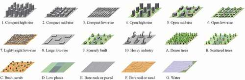
The city plays an important role in the developing process of human society. Urbanization is one of the most principal phenomena in the world today (Li et al. 2019; Shen et al. 2020; Wu, Gui, and Yang 2020; Zhou, Zhai, and Yu 2020). In the process of urbanization, the size of city expands at the expense of occupying agricultural land and green open space (Hadeel, Jabbar, and Chen 2009; Huang and Wang 2020; Shao et al. 2020), and the mass population assembles to the city (Li, Zhao, and Li 2016; Trinder and Liu 2020; Shao et al. 2021). The cities are under pressure from increasing population and ecological threats as a result of rapid urbanization (Alsaaideh et al. 2017). UHI effect is one of the most significant environmental issues caused by urbanization (Yang et al. 2020). UHI refers to the phenomena that urban areas are warmer than the surrounding suburban areas. Most researchers assessed the UHI intensity through a classical urban-rural temperature difference (Jiang, Chen, and Jing 2006; Zeng et al. 2010; Oke and Stewart 2012; Yang et al. 2020; Zhou et al. 2020a; Huang, Liu, and Li 2021). However, due to the absence of universal definitions for urban or rural, it’s not easy to qualify a site as urban or rural. UHI research has long been limited by the urban-rural classification. LCZ classification scheme is introduced to address this problem (Oke and Stewart 2012). The LCZ is a classification scheme that provides a standardization framework to present the characteristics of urban forms and functions (Oke and Stewart 2012; Bechtel et al. 2015; Qiu et al. 2020). LCZs are defined as regions of uniform surface cover, structure, material, and human that span hundreds of meters to several kilometers on a horizontal scale (Oke and Stewart 2012). The LCZ scheme consists of ten built types and seven land cover types. Each LCZ type represents a culturally neutral description of a specific urban landscape based on its effect on the local air temperature (Mills et al. 2015). Illustrations of the LCZ classes are displayed in Figure 1. The LCZ scheme is originally designed for UHI research (Oke and Stewart 2012), but has shown an increasing impact on various climatological studies that include estimating nocturnal cooling effect (Leconte, Bouyer, and Claverie 2020), climate-sensitive street design (Maharoof, Emmanuel, and Thomson 2020), and analyzing urban ventilation (Yang et al. 2019; Zhao et al. 2020).

Figure 1. Illustrations of LCZ classes.

Recent efforts have been focusing on the development of LCZ mapping techniques. The World Urban Database and Portal Tool (WUDAPT) proposed a method that employs Landsat data and open source software for worldwide LCZ mapping (Oke and Stewart 2012; Bechtel et al. 2015; Mills et al. 2015; Cai et al. 2016; Danylo et al. 2016; Ching et al. 2018; Bechtel et al. 2019). The WUDAPT method, which has been applied in many studies (Cai et al. 2016; Danylo et al. 2016; Cai et al. 2018; Shi et al. 2019; Zhou et al. 2020b; Shi et al. 2021), needs experts with local knowledge of individual city to build reference polygons using Google Earth. These polygons are applied to train and test LCZ classification models with Landsat images (resampled into 100 m resolution). Random Forest (RF), a rule-based machine learning approach, is further used for classification in WUDAPT. Despite its popularity, WUDAPT is a pixel-based classification method that largely ignores spatial information, thus leading to relatively low accuracy (Qiu et al. 2020).

To achieve high accuracy, other LCZ mapping methods have been investigated, one notable effort of which is the Geographic Information System (GIS) stream. GIS-based methods use GIS datasets, such as building footprints and high-resolution digital surface models, to obtain parameters that are applied to define LCZ types (Zheng et al. 2018; Oliveira, Lopes, and Niza 2020). GIS-based methods are able to improve the LCZ classification accuracy but require massive input datasets that are not always available to the public (Quan and Bansal 2021).

In recent years, deep learning approaches have been widely adopted in remote sensing image scene classification and achieved state-of-the-art classification accuracy (Cheng et al. 2020). Liu and Shi (2020) pointed out that LCZ mapping can be regarded as a scene classification task to fully exploit the contextual information from remote sensing images. With the growing popularity of deep learning, many scholars have investigated the potential of deep learning algorithms in LCZ mapping. Deep learning methods, especially in the form of CNNs, are expected to further boost LCZ classification accuracy. Huang, Liu, and Li (2021) proposed a novel CNN model to generate LCZ classification results using Landsat imagery for China’s 32 major cities, and satisfactory classification accuracies in 32 cities were achieved by the proposed model. Zhu et al. (2020) developed a big benchmark dataset, So2Sat LCZ42, that contains Sentinel-1 and Sentinel-2 image patch pairs and LCZ labels from 42 cities in different countries. This dataset is openly available and is regarded as a standard dataset for deep learning-based LCZ mapping. Qiu et al. (2020) proposed a CNN framework, termed as Sen2LCZ-Net, to classify LCZs using Sentinel-2 images from the So2Sat LCZ42 dataset. Liu and Shi (2020) selected 15 cities in three economic regions of China and used Sentinel-2 data to classify LCZs by employing the proposed LCZNet composed of residual learning and SE block. The effect of image size was investigated, and the results showed that an image size of 48 × 48 (corresponding to 480 × 480 m²) obtained the highest accuracy (Liu and Shi 2020). The aforementioned studies used multispectral images only. SAR, another typical remote sensing sensor, is sensitive to moisture and geometric characteristics and can provide useful information different from multispectral images (Li and Zhang 2014; Shao, Wu, and Guo 2020). The potential of SAR data for LCZ mapping has been studied in recent work. Bechtel et al. (2016) found that individual SAR amplitude and range helped improve LCZ classification accuracy slightly. Demuzere, Bechtel, and Mills (2019) compared Sentinel-1 backscatter, entropy, and Geary C using random forest and found that Sentinel-1 backscatter was most informative (via feature importance ranking). Hu, Ghamisi, and Zhu (2018) compared numerous Sentinel-1 SAR components using canonical component analysis and found features related to VH polarized data contributed the most to LCZ classification. Feng et al. (2019) employed both SAR and multispectral data of the So2Sat LCZ42 dataset for CNN-based LCZ mapping and achieved improved accuracy. Jing et al. (2019) revealed the contributions of the SAR data and the multispectral data of the So2Sat LCZ42 dataset to the LCZ classification performance. Their study suggested that the combination of SAR and multispectral data contributes to improved LCZ classification accuracy, however, in an unnoticeable manner.

Sentinel-1 data of the So2Sat LCZ42 dataset contain eight channels, including four elements of VH and VV intensity images and four elements of the Refined LEE filtered result (Zhu et al. 2020). La, Bagan, and Yamagata (2020) pointed out that decomposed components of SAR data can also enhance the LCZ mapping performance using supervised pixel-based methods. To our best knowledge, few efforts have been made that focus on the effect of backscattering characteristics of SAR data on the performance of deep learning-based LCZ mapping.

In this study, we employ openly available Sentinel-1 SAR data and Sentinel-2 multispectral imagery to classify LCZs. We propose a deep CNN architecture, termed as RSNNet, for LCZ mapping in three large cities (Beijing, Tianjin, and Wuhan) in China and further investigate the LCZ classification results. Finally, we analyze the effect of different backscattering characteristics of SAR data on the accuracy of LCZ mapping. The rest of this article is organized as follows. Section 2 introduces the study area and Sentinel data. Section 3 elaborates on the proposed network, RSNNet, and the details of network training. Section 4 presents the classification results. Section 5 discusses the effect of input bands on classification accuracy and compares the proposed network with other networks. Finally, Section 6 concludes this article.

2. Study areas and datasets

2.1. Study areas

Three large cities in China, Beijing, Tianjin and Wuhan, were selected for our study. Their geographical locations are shown in Figure 2

Figure 2. Locations of Beijing, Tianjin and Wuhan in China (a); Sentinel-2 image of Beijing (b), Tianjin (c), and Wuhan (d) .

. Population, area and Gross Domestic Product (GDP) in 2019 of the selected three cities are displayed in Table 1.

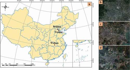
Table 1. Population, area, and GDP of the three selected cities.

City	Population (10^3)	Area (km^2)	GDP (10^6 RMB)
Beijing	21,536	16,410.54	3,537,130
Tianjin	15,618.3	11,966.45	1,410,428
Wuhan	11,212	8569.15	1,622,321

The city of Beijing, covering 16,410 km², is the capital of China. It is located at the northern end of the North China Plain. Beijing has a typical monsoon-driven semi-humid to humid continental climate, characterized by hot and humid summer and cold and dry winter. It has been a highly urbanized city with preserved historic buildings, such as Siheyuan, which can be categorized into compact low-rise (LCZ 3). As heavy industrial factories (LCZ 10) were relocated from Beijing to its neighboring cities, Beijing now has only a few LCZ 10.

The city of Tianjin, one of the megacities in China, is located in the northeast of North China Plain and borders the Bohai Sea in the east. It covers an area of 11,966 km² (plains account for 93%). Tianjin is a city that has a large number of factories with strong industrial activities (LCZ 8 and LCZ 10).

Wuhan is the capital city of the Hubei Province, China, situated in central China. The Yangtze, the world’s third longest river, and its largest tributary Hanshui meet in Wuhan and cut the city into three parts: Hankou, Hanyang and Wuchang. Wuhan has a humid subtropical climate with four distinct seasons. Wuhan consists of many rivers and lakes (LCZ G) with water bodies covering 2217 km² (accounting for 26.1% of the total area of Wuhan).

2.2 Datasets and pre-processing

2.2.1 Sentinel-1 data

Sentinel-1 is a C-band synthetic aperture radar satellite and comprises a constellation of two polar-orbiting satellites (Sentinel-1A and Sentinel-1B) (Abdel-Hamid, Dubovyk, and Greve 2021). The Sentinel-1 mission provides a public global SAR dataset. We acquired Sentinel-1VV-VH dual-Pol Single-Look Complex (SLC) level 1 data that covers the three selected cities from the Copernicus Open Access Hub. Sentinel-1 images were acquired on 14 August 2019 (Beijing), 21 August 2019 (Tianjin) and 12 August 2019 (Wuhan). The European Space Agency’s Sentinel Application Platform was used for the preprocessing of Sentinel-1 data. Figure 3 displays the flowchart of Sentinel-1 data preprocessing. The specific steps are listed as follows.

Figure 3. Flowchart of Sentinel-1 SAR data preprocessing.

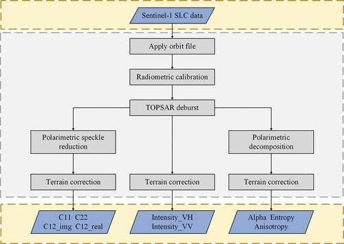
(1) The implementation of orbit file: This is the first step of any SAR preprocessing. A precise orbit file is used to improve the geocoding of the product.

(2) Radiometric calibration: The operator computes the backscatter intensity using sensor calibration parameters in the metadata.

(3) TOPSAR deburst: The Sentinel-1 IW products contain three sub-swaths for each polarization channel. Each sub-swath image has a series of bursts. The TOPSAR deburst operator can remove the seamlines between the single bursts and merge these bursts and sub-swaths into a SLC image.

(4a) Polarimetric speckle reduction: Speckle filters aims to reduce the number of speckles. The Refined Lee speckle filter was selected to conduct the speckle reduction.

(4b) Polarimetric decomposition: Sentinel-1 has only two polarizations: HH and VH. H-Alpha Dual Pol decomposition was applied to obtain Alpha, Anisotropy, and Entropy.

(5) Terrain correction: Terrain correction geocodes the image by correcting SAR geometric distortions using a Digital Elevation Model (DEM) and producing a projected product. The SRTM DEM was selected as input DEM to accomplish the correction. The WGS84/UTM coordinate system was applied to geocode the product, and the images were upsampled to 10 m Ground-Sampling Distance (GSD).

After preprocessing, the outputs include two intensity images (Intensity_VH and Intensity_VV), three polarimetric decomposition components (Alpha, Anisotropy, and Entropy) and four polarimetric speckle reduction components (C11, C22, C12_img, and C12_real). The Sentinel-1 data in the dataset we build in this paper contain nine bands, which is displayed in Table 2.

Table 2. Band names of Sentinel-1 and Sentinel-2 data in Sen12LCZ dataset.

No.	Sentinel-1	Sentinel-2
1	Alpha	B2
2	Anisotropy	B3
3	Entropy	B4
4	C11	B5
5	C12_img	B6
6	C12_real	B7
7	C22	B8
8	Intensity_VH	B8a
9	Intensity_VV	B11
10	\	B12

2.2.2 Sentinel-2 data

Google Earth Engine (GEE) was employed to obtain cloud-free Sentinel-2 images (Schmitt et al. 2019). The overall workflow, implemented via the GEE Python Application Programming Interface (API), included three main modules.

(1) Query Module: loading images from the catalog.

(2) Quality Score Module: calculating a quality score for each image.

(3) Image Merging Module: mosaicking selected images based on the meta-information generated in the preceding modules.

Consistent with Sentinel-1 data, the acquisition time of Sentinel-2 data was set as Summer (1st June till 31st August). This workflow of GEE-based procedure for cloud-free Sentinel-2 image generation uses multi-temporal information of comparably short time periods to obtain cloud-free Sentinel-2 data, which means that the dates of Sentinel-1 imaging and the dates of Sentinel-2 imaging are not an exact match. Although the acquisition dates of Sentinel-1 and Sentinel-2 sets are different, they are very close. Generally, the form and structure of urban buildings do not change greatly within a few months, and the state of vegetation may change. In this study, we consider the difference between the dates of Sentinel-1 imaging and the dates of Sentinel-2 imaging as acceptable.

Sentinel-2 images consist of thirteen spectral bands, including four bands (B2, B3, B4, B8) with 10 m GSD, six bands (B5, B6, B7, B8a, B11, B12) with 20 m GSD, and three bands (B1, B9, B10) with 60 m GSD. In the study, bands with 60 m GSD were discarded. Bands with 20 m GSD were resampled to 10 m GSD via the nearest neighbor algorithm. The Sentinel-2 data in the Sen12LCZ dataset consist of 10 bands with 10 m GSD.

2.2.3 Preparing label data

Label data were collected on Google Earth following the standard procedure defined in the WUDAPT project (Ching et al. 2018). First, a region of interest within each selected city was defined by drawing a rectangle of about 50 × 50 km² around the city center in Google Earth. We further delineated polygons that enclosed different LCZ types. We ensure that each LCZ type has more than five polygons and there are enough samples for each category. Each polygon must be wider than 200 m to avoid interference of small landscape, such as an individual building.

2.3 Sen12LCZ dataset

The dimension of the image patch has a great impact on classification accuracy. It has been proved that a large scene is beneficial for LCZ mapping, as a large input size can provide additional urban environmental features (Liu and Shi 2020). Sentinel-1 and Sentinel-2 images were used to create a dataset named “Sen12LCZ”, and the dimension of the Sentinel-1 and Sentinel-2 image patches was defined as 48 × 48, corresponding to an area of 480 × 480 m².

The labeled polygons were sampled using a 480 m by 480 m fishnet, and the center of each grid in the fishnet corresponds to the center of each image patch. When the center of a grid fell within a polygon, we labeled the corresponding grid as the category to which the polygon belongs. We extracted Sentinel-1 and Sentinel-2 image patch pairs with the corresponding LCZ labels by projecting the sampled label data to the registered Sentinel-1 and Sentinel-2 images. Finally, a total of 4083 pairs of image patches were obtained. Table 3 displays the specific number of image pairs for each selected city corresponding to different LCZ types. The number of all image pairs in the dataset is 4083. The dataset was further split into a training set (60%), a testing set (20%), and a validation set by adopting stratified sampling strategy. These three sets consist of 2611, 818 and 654 pairs of image patches, respectively.

Table 3. The number of image pairs corresponding to different LCZ types in Beijing, Wuhan, Tianjin and sums of three cities.

LCZ Type	Beijing	Wuhan	Tianjin	Sum
1	28	19	9	56
2	57	56	21	134
3	112	40	121	273
4	96	80	60	236
5	120	83	93	296
6	75	41	16	132
7	29	6	3	38
8	113	153	89	355
9	40	12	7	59
10	42	90	75	207
A	140	91	3	234
B	78	38	38	154
C	40	68	62	170
D	150	153	248	551
E	54	18	15	87
F	57	84	163	304
G	82	270	445	797
Total	1313	1302	1468	4083

3. Methods

3.1 The proposed network

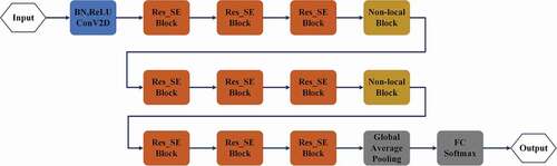
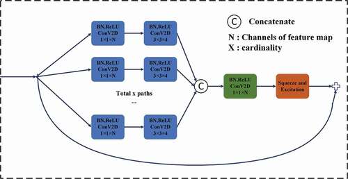
In this study, we proposed a network named RSNNet for LCZ mapping. Figure 4 illustrates the architecture of the proposed RSNNet that includes several Res_SE blocks and non-local blocks. Res_SE block consists of a building block of ResNeXt and a SE block. SE block can integrate channel-wise features by squeezing less important features and excite the useful feature maps (Hu et al. 2020). Every three consecutive Res_SE blocks form a stage. Features extracted from the first and the second stage go through a non-local block. At the end of the last block, a global average pooling layer is applied, followed by a fully connected layer with a softmax classifier for the final prediction. Note that samples in each LCZ type are imbalanced (Table 3). Studies have proved that sample imbalance tends to have negative impacts on classification performance (Chakraborty et al. 2020; Wu et al. 2020; Zhang et al. 2021). To address this issue, we applied focal loss to the proposed CNN (details in Section 3.4).

Figure 4. The architecture of the proposed RSNNet.

3.2 Res_SE block

Res_SE block in the proposed network includes a building block of ResNeXt and a SE block. Figure 5 depicts the structure of the Res_SE block. ResNeXt adopts the repeating-layer strategy from VGG and ResNets and exploits the split-transform-merge strategy. The concept of cardinality (the size of the set of transformations) is also introduced in ResNeXt. The basic module of ResNeXt consists of the following operations.

1. Splitting: The first 1 × 1 layer of each branch produces the low-dimensional embedding.

2. Transforming: The low-dimensional representation is transformed via 3 × 3 layers.

3. Aggregating: The transformations of all branches are first concatenated together and then serve as input to the 1 × 1 layer with Batch Normalization (BN) and Rectified Linear Unit (ReLU) function. The shortcut connection is also employed.

Figure 5. Structure of the Res_SE block.

As a key unit in SENet, SE block that achieves dynamic channel-wise feature enhancement by selectively emphasizing informative features and suppress less useful ones (Hu et al. 2020) is stacked in the building block of ResNeXt. During the squeezing process, global average pooling is applied for a feature map $U\in {\mathbb{R}}^{H\times W\times C}$ to generate channel-wise statistics $z\in {\mathbb{R}}^C$:

(1) $z_C=F_{\mathrm{s}\mathrm{q}}(U_C)=\frac{1}{H\times W}\sum _{i=1}^H\sum _{j=1}^W{u}_C(i,j)$(1)

where $U_C$ refers to a 2D feature map of channel $C$ with a spatial dimension $H\times W$, $F_{\mathrm{s}\mathrm{q}}$ is the squeeze process, $u_c$ is the value of $(x,y)$ and $z_c$ is the channel-wise statistics of the $C-\mathrm{t}\mathrm{h}$ feature map.

The excitation process aims to fully capture channel-wise dependencies. A simple gating mechanism with a sigmoid activation is employed to fulfill this objective:

(2) $s=F_{\mathrm{e}\mathrm{x}}(z,L)=\sigma (L_2\delta (L_{1}z))$(2)

where $F_{\mathrm{e}\mathrm{x}}$ is the excitation process, $\sigma$ refers to the sigmoid function, $\delta$ is the ReLU function, $L_1$ and $L_2$ refer to fully connected layers.

The final output of the SE block is obtained by multiplying a scalar $s$ and the original feature map $U$:

(3) $y_C=F_{\mathrm{s}\mathrm{c}\mathrm{a}\mathrm{l}\mathrm{e}}(u_C,s_C)=s_C{u}_C$(3)

where $F_{\mathrm{s}\mathrm{c}\mathrm{a}\mathrm{l}\mathrm{e}}$ is channel-wise multiplication between the scalar $s_C$ and the feature map $u_C\in {\mathbb{R}}^{H\times W}$.

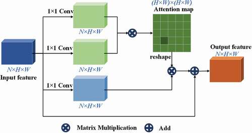
3.3 Non-local block

A non-local block is capable of capturing long-range dependencies (Wang et al. 2018). The structure of the non-local block is displayed in Figure 6. Non-local operations maintain the variable input sizes and can be easily applied to other networks. In this study, we employ non-local blocks to capture long-range contextual information, aiming to further improve classification accuracy.

Figure 6. The structure of the non-local block.

3.4 Focal loss

Proposed by Lin et al. (2017), the focal loss function considers the extreme imbalance between easy and hard samples as well as between positive and negative samples. A modulating factor is added to the Cross-Entropy (CE) loss to focus training on hard negatives in the focal loss.

The original focal loss is designed for binary classification. Further, it has been adopted to handle multi-class tasks. The CE loss for multi-class cases is defined as (Liu, Chen, and Chen 2018):

(4) $\mathrm{C}\mathrm{E}=-\sum _{i=1}^M{t}_{i}log\left(y_i\right)$(4)

where $M$ refers to the number of categories, $t_i$ is a real probability distribution, $y_i$ denotes the probability distribution of prediction. $t_i$ is defined as:

(5) $t_i=\left\{\begin{array}{c}1\\ 0\end{array}\right.\begin{array}{c}i\mathrm{i}\mathrm{s}\mathrm{t}\mathrm{r}\mathrm{u}\mathrm{e}\mathrm{l}\mathrm{a}\mathrm{b}\mathrm{e}\mathrm{l}\\ i\mathrm{i}\mathrm{s}\mathrm{n}\mathrm{o}\mathrm{t}\mathrm{t}\mathrm{r}\mathrm{u}\mathrm{e}\mathrm{l}\mathrm{a}\mathrm{b}\mathrm{e}\mathrm{l}\end{array}$(5)

To address the issue of class imbalance, focal loss adds a modulating factor ${\left(1-y_i\right)}^{\gamma }$ and a weighting factor ${\alpha }_i\in \left[0,1\right]$ to the CE loss, with a tunable focusing parameter $\gamma \ge 0$. The multi-class focal loss is defined as:

(6) $\mathrm{F}\mathrm{L}=-\sum _{i=1}^M{\alpha }_i{\left(1-y_i\right)}^{\gamma }{t}_{i}log\left(y_i\right)$(6)

In this study, $\alpha$ is set by inverse class frequency. The focus parameter $\gamma$ is employed to control the rate at which easy-classified examples are down-weighted. When $\gamma =0$, FL is equivalent to CE. The effect of the modulating factor also increases along with the increase of $\gamma$. Here, we set $\gamma =2$ for RSNNet after a trial-and-error process, and we display the experimental results in Section 5.3.

3.5 Metrics for accuracy assessment

We adopted OA, Average Accuracy (AA), Kappa coefficient, Producer’s Accuracy (PA) and User’s Accuracy (UA) for performance evaluation in this study. These metrics are calculated as:

(7) $\mathrm{O}\mathrm{A}=\frac{1}{N}\sum _{i=1}^M{x}_{ii}$(7)

(8) $\mathrm{A}\mathrm{A}=\frac{\sum _{i=1}^M\frac{x_{ii}}{x_{i+}}}{M}$(8)

(9) $\mathrm{K}\mathrm{a}\mathrm{p}\mathrm{p}\mathrm{a}=\frac{N\sum _{i=1}^M{x}_{ii}-\sum _{i=1}^M(x_{i+}\times x_{+i})}{N^2-\sum _{i=1}^M(x_{i+}\times x_{+i})}$(9)

(10) $\mathrm{P}{\mathrm{A}}_i=\frac{x_{ii}}{x_{i+}}$(10)

(11) $\mathrm{U}{\mathrm{A}}_i=\frac{x_{ii}}{x_{+i}}$(11)

where $N$ refers to the amount of samples applied for accuracy measurement, $M$ is the number of categories, $x_{ii}$ refers to the number of units that come from class $i$ and predicted as class $i$, $x_{i+}$ denotes the number of samples in class $i$, $x_{+i}$ is the number of samples predicted as class $i$.

3.6 Network training strategy

The experiments were conducted on Python 3.5 using Keras with TensorFlow backend. The Nesterov Adam optimizer was applied to train the network. We set the batch size to 16 and the initial learning rate to 0.002 (decreased by half after every five epochs). To avoid overfitting and to control the training time, we employed early stopping. Validation with patience of 50 epochs loss was chosen as the monitored metric.

4. Results

4.1 LCZ classification results in three selected cities

RSNNet was trained and tested using the label data obtained from the same city to classify three cities respectively. We set the parameters to the same, only the input training data and testing data were different.

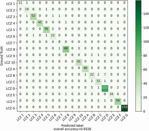
The confusion matrix in Beijing is displayed in Figure 7(a). The classification model we proposed, RSNNet, achieves an OA of 0.9202 and a Kappa coefficient of 0.9138. Urban classes are generally well classified. However, the confusion still exists. LCZ A (dense trees) and LCZ G (water) are easily identified. LCZ B (scattered trees) is confused with LCZ C (bush, scrub). The confusion matrix in Tianjin is presented in Figure 7(b). Our proposed RSNNet achieves an OA of 0.9524 and a Kappa coefficient of 0.9436. Similar to the classification results in Beijing, most LCZ classes are well classified in Tianjin, whereas confusion still exists among certain classes. Classification of Wuhan by our proposed RSNNet achieves an OA of 0.9004 and a Kappa coefficient of 0.8891. The confusion matrix of Wuhan is presented in Figure 7(c). we notice that LCZ 2 are confused with LCZ 3 and LCZ 1. LCZ G is the easiest LCZ type to classify. We also trained the proposed network using data from all three cities. The confusion matrix of this experiment is presented in Figure 8. Our proposed RSNNet achieves an OA of 0.9328 and a Kappa coefficient of 0.9257. The main misclassifications are between LCZ 1 and LCZ 4, LCZ 2 and LCZ 3, LCZ 4 and LCZ 5, LCZ C and LCZ D, and LCZ B and LCZ D. We observe that LCZ G is the most distinct LCZ type, as our RSNNet achieves 100% accuracy in classifying this LCZ type.

Figure 7. Confusion matrix of Beijing, Tianjin and Wuhan.

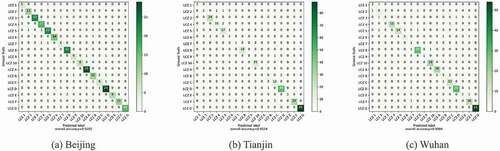
Figure 8. Confusion matrix of all data of three cities.

4.2 LCZ maps

LCZ classification maps of Beijing, Tianjin, and Wuhan and the corresponding Sentinel-2 images are shown in Figure 9. In general, these classification maps present unique urban fabrics in these cities. For Beijing, LCZ 3 (compact low-rise), LCZ 2 (compact mid-rise), and LCZ 4 (open high-rise) are the dominant types in the urban regions. A large area of LCZ A (dense trees) is identified in Figure 9(a) due to the existence of mountains in the northeastern Beijing.

Figure 9. LCZ maps and the corresponding Sentinel-2 images of Beijing (a), Tianjin (b) and Wuhan (c).

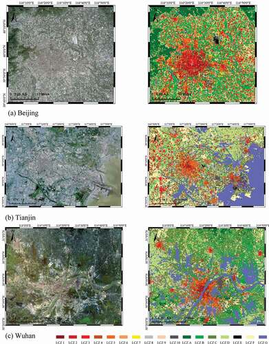
As for Tianjin, LCZ 1 (compact high-rise) and LCZ 3 (compact low-rise) are observed in the central urban area. The entire urban region is mostly covered by LCZ 4 (open high-rise) and LCZ 5 (open mid-rise). There are many LCZ 8 (large low-rise) in the suburban areas. The existence of idle farmland in Tianjin leads to the identification of LCZ F (bare soil or sand) on the west side of Tianjin. A large area of LCZ D (low plants) is also notable in eastern Tianjin.

For Wuhan, the Yangtze River and many lakes can be easily identified in the classified LCZ map. The major LCZ types in urban regions of Wuhan are LCZ 4 and LCZ 5. The heavy industrial area in the northern suburban region is clearly presented. Hills covered by forests in the urban region are classified as LCZ A.

In summary, we observe that the urban structure of these three study areas is well identified and clearly presented using the Sen12LCZ dataset via the proposed network.

UHI magnitude is defined as an “urban-rural” difference in most previous studies:

(12) $\mathrm{U}\mathrm{H}{\mathrm{I}}_{\mathrm{u}-\mathrm{r}}=T_{\mathrm{u}\mathrm{r}\mathrm{b}\mathrm{a}\mathrm{n}}-T_{\mathrm{r}\mathrm{u}\mathrm{r}\mathrm{a}\mathrm{l}}$(12)

where $\mathrm{U}\mathrm{H}{\mathrm{I}}_{\mathrm{u}-\mathrm{r}}$ refers to the magnitude of UHI, $T_{\mathrm{u}\mathrm{r}\mathrm{b}\mathrm{a}\mathrm{n}}$ and $T_{\mathrm{r}\mathrm{u}\mathrm{r}\mathrm{a}\mathrm{l}}$ refer to the temperature of urban and rural areas respectively.

Local climate zone is proposed to redefine UHI magnitude in an LCZ temperature difference (Oke and Stewart 2012):

(13) $\mathrm{U}\mathrm{H}{\mathrm{I}}_{\mathrm{L}\mathrm{C}\mathrm{Z}\mathrm{x}}=T_{\mathrm{L}\mathrm{C}\mathrm{Z}\mathrm{x}}-T_{\mathrm{L}\mathrm{C}\mathrm{Z}\mathrm{D}}$(13)

where $\mathrm{U}\mathrm{H}{\mathrm{I}}_{\mathrm{L}\mathrm{C}\mathrm{Z}\mathrm{x}}$ denotes the magnitude of UHI for LCZ x, $T_{\mathrm{L}\mathrm{C}\mathrm{Z}\mathrm{x}}$ refers to the temperature of LCZ x, and $T_{\mathrm{L}\mathrm{C}\mathrm{Z}\mathrm{D}}$ refers to the temperature of LCZ D (low plants).

Due to the complex land surface components, it is difficult to accurately discriminate urban and rural areas. LCZ temperature differences are more conducive to analysis, because the standardized description of surface structure and cover is highlighted in this climate-based classification scheme.

For deriving the intensity of UHI in an LCZ temperature difference, the thermometric network design is important. There should be thermometers in each LCZ type, and the number of sensors of each type should be proportional to the area of each type. To avoid the effect of changes in airflow and stability conditions on air temperature, the thermometers are forbidden to locate on or near the border of two zones. Thermometric networks in different cities should be designed with reference to their LCZ maps. For instance, there are many LCZ 8 and LCZ 10 in Tianjin, and many thermometers should be uniformly placed on these areas. However, LCZ 8 and LCZ 10 are few in Beijing, and only a few sensors are needed for LCZ 8 and LCZ 10.

5. Discussion

5.1 Effect of input bands

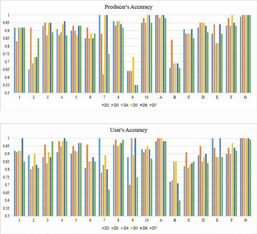
Sen12LCZ dataset consists of a total of 19 channels, including nine features obtained from Sentinel-1 SAR data and ten bands of Sentinel-2 multispectral imagery. In this study, seven datasets, designated as D1-D7, were set up to explore the effect of different combinations of multi-source data on LCZ classification (Table 4). D1 includes nine features extracted from Sentinel-1 data. D2 consists of 10 bands of Sentinel-2 images alone. D3 adds three decomposed components (Alpha, Anisotropy, and Entropy) to D2. D4 integrates additional four elements obtained from the Refined LEE filter operation (C11, C12_img, C12_real, and C22) to D2. D5 adds intensity channels of VH and VV to D2. D6 includes all 19 channels from Sentinel-1 and Sentinel-2 data. D7 consists of three Sentinel-1 components in D3, two Sentinel-1 components in D5 and 10 bands of D2.

Table 4. Classification accuracy with different input combinations.

Dataset	Bands	Data source	Components	OA	Kappa	AA
D1	9	Sentinel-1	Alpha Anisotropy Entropy C11 C12_img C12_real C22 Intensity_VH Intensity_VV	0.3790	0.3040	0.1739
D2	10	Sentinel-2	Band2-8, 8a, 11, 12	0.9181	0.9095	0.9055
D3	13	Sentinel-1	Alpha Anisotropy Entropy	0.9425	0.9366	0.9060
		Sentinel-2	Band2-8, 8a, 11, 12
D4	14	Sentinel-1	C11 C12_img C12_real C22	0.9132	0.9039	0.8990
		Sentinel-2	Band2-8, 8a, 11, 12
D5	12	Sentinel-1	Intensity_VH Intensity_VV	0.9340	0.9270	0.9155
		Sentinel-2	Band2-8, 8a, 11, 12
D6	19	Sentinel-1	Alpha Anisotropy Entropy C11 C12_img C12_real C22 Intensity_VH Intensity_VV	0.9328	0.9257	0.9184
		Sentinel-2	Band2-8, 8a, 11, 12
D7	15	Sentinel-1	Alpha Anisotropy Entropy Intensity_VH Intensity_VV	0.9315	0.9244	0.8928
		Sentinel-2	Band2-8, 8a, 11, 12

The proposed RSNNet was separately trained on these datasets, and the classification accuracy metrics are presented in Table 4. The results suggest that SAR data do not contain enough information for LCZ classification, evidenced by the low accuracy of D1 (Sentinel-1 only). D2 achieves an OA of 0.9181, a Kappa coefficient of 0.9095 and an AA of 0.9055. As expected, the addition of SAR data to multispectral bands enhances the LCZ classification performance. As shown in Table 4, D3 achieved the highest accuracy, with OA, Kappa coefficient, and AA of 0.9425, 0.9366 and 0.9060, respectively. The above results show that the decomposition method is an efficient tool to extract structure and scattering information which can be combined with multispectral data to improve classification performance (Lee and Pottier 2009).

The classification result of D4 is quite close to D2, suggesting that the information contained in Refined Lee filter components benefits LCZ mapping in a trivial manner. The OA, Kappa, and AA of D5 are 0.9340, 0.9270, and 0.9155, respectively, which are higher than D2, suggesting that the intensity of VV and VH greatly contribute to LCZ mapping. D6 achieves an OA of 0.9328, which is lower than D3 and D5 but higher than D2. As D6 contains information from all 19 channels, its data redundancy leads to reduced accuracy in the LCZ classification compared to D3 or D5. We combined the Sentinel-1 components in D3 and D5 with ten bands of D2 as a new dataset which was designated as D7. RSNNet was trained and tested on D7. D7 achieves an OA of 0.9315, which is lower than D3 and D5, suggesting that the combination of superior datasets leads to lower accuracy. Considering the great performance of D3, we can conclude that the decomposed components contribute more than filtered components and intensity channels.

To analyze the influence of SAR characteristics on individual class, we present PA and UA obtained with different datasets in Figure 10

Figure 10. PA and UA of classified LCZ with different datasets.

. The results indicate that LCZ A and LCZ G can be easily identified, evidenced by their high PAs and UAs. Compared with natural land cover types, the classification of built-up types benefits more from SAR characteristics. For LCZ 2, the PAs obtained from D3, D4, D5, and D6 are higher than D2. Similarly, for LCZ 3, the PAs and UAs obtained from D3, D5, and D6 are higher than D2.

The Sentinel-1 SAR data used in this study are in double (VV-VH) polarization. Thus only H-Alpha Dual Pol decomposition can be used to extract decomposed components. The fully polarimetric SAR data can provide more backscattering information than Sentinel-1 data, and many different target decomposition methods have been developed to transform backscattering information into basic backscattering mechanisms (Touzi, Boerner, and Lueneburg 2004; Yamaguchi, Yajima, and Yamada 2006). As fully polarimetric SAR data offers more capacity in terrain classification (Kajimoto and Susaki 2013; Angelliaume et al. 2018), future efforts can be made to integrate fully polarimetric SAR data with multispectral data in deep learning-based LCZ mapping.

5.2 Comparison with other CNNs

Table 5 presents the classification results of our proposed RSNNet and other popular CNNs, such as ResNet, DenseNet, Sen2LCZ-Net proposed by Qiu et al. (2020), MSCNN built by Kim et al. (2020) and CNN constructed by Yoo et al. (2019). ResNet, which won 1st place on the ILSVRC 2015 classification task, introduce the design of shortcut connections to alleviate vanishing gradients (He et al. 2016). DenseNet connects each layer to every other layer in a feed-forward fashion and obtains significant improvements in various image segmentation and classification tasks (Huang et al. 2017). Sen2LCZ-Net is a simple CNN that considers multilevel feature fusion for LCZ mapping and achieves great performance in LCZ classification using the So2Sat LCZ42 dataset (Qiu et al. 2020). MSCNN was used to evaluate LCZ classification accuracy with the custom LCZ training data (Kim et al. 2020). Yoo et al. (2019) constructed CNN to compare CNN with random forest classifier for LCZ classification.

Table 5. Performance comparison among ResNet-50, DenseNet-121, Sen2LZC-Net(f16D17), LCZNet, MSCNN, CNN (Yoo et al. 2019), and the proposed RSNNet.

CNNs	Metrics
	OA	Kappa	AA
ResNet-50	0.9144	0.9055	0.8954
DenseNet-121	0.8826	0.8703	0.8091
Sen2LCZ-Net(f16D17)	0.8142	0.7936	0.7513
LCZNet	0.9022	0.8920	0.8665
MSCNN	0.8056	0.7848	0.6741
CNN (Yoo et al. 2019)	0.7885	0.7649	0.6363
RSNNet	0.9328	0.9257	0.9184

In this table, the bold indicates the best result.

D6 including all 19 channels from Sentinel-1 and Sentinel-2 data was used to train the proposed RSNNet and other CNNs. Although D6 contains more information than other datasets, it is not the best-performing dataset in Section 5.1 due to its data redundancy. By applying the non-optimal dataset to train the models, the ability of different CNNs to extract representative features from all 19 bands of Sentinel-1 and Sentinel-2 data can be better compared.

The results suggest that the proposed RSNNet which integrates spatial attention module and channel attention module achieves the best performance in all three metrics, with OA, Kappa and AA being 0.9328, 0.9257 and 0.9184, respectively. In comparison, the classification result by CNN is the worst (OA: 0.7885; Kappa: 0.7649; AA: 0.6363). The above results prove the superiority of RSNNet over selected widely-adopted CNNs.

5.3 Effect of focal loss

As mentioned in Section 2.3, samples of each category in the Sen12LCZ dataset are imbalanced (see Table 3). To eliminate the impact of the imbalanced dataset on classification accuracy, we implement focal loss in this study. The focus parameter $\gamma$ has an effect on the performance of focal loss. Table 6 displays the effect of different $\gamma$ values on LCZ classification accuracy when focal loss is implemented in ResNet, DenseNet, Sen2LCZ-Net and RSNNet. D6 was used to train the models. The experimental results suggest that different networks have different optimal $\gamma$ values. The best result for RSNNet is obtained when $\gamma$ is set as 2. For ResNet-50, the optimal $\gamma$ value is 3.

Table 6. Performance comparison in ResNet, DenseNet, Sen2LZC-Net, and RSNNet with different $\gamma$ values.

CNNs	$\gamma$	Metrics
		OA	Kappa	AA
ResNet-50	0	0.9193	0.9107	0.8973
	1	0.9181	0.9095	0.8869
	2	0.9144	0.9055	0.8954
	3	0.9267	0.9188	0.9137
	4	0.9083	0.8985	0.8798
	5	0.9144	0.9053	0.9050
	6	0.9218	0.9135	0.9171
DenseNet-121	0	0.8619	0.8473	0.7924
	1	0.8912	0.8799	0.8505
	2	0.8826	0.8703	0.8091
	3	0.8826	0.8704	0.8346
	4	0.8704	0.8569	0.8019
	5	0.8851	0.8729	0.8338
	6	0.8826	0.8702	0.8104
Sen2LCZ-Net(f16D17)	0	0.8215	0.8011	0.7298
	1	0.8203	0.8007	0.7230
	2	0.8142	0.7936	0.7513
	3	0.8044	0.7833	0.6913
	4	0.8227	0.8029	0.7015
	5	0.8337	0.8153	0.7819
	6	0.8166	0.7962	0.7262
RSNNet	0	0.8900	0.8783	0.8380
	1	0.8863	0.8744	0.8296
	2	0.9328	0.9257	0.9184
	3	0.9083	0.8987	0.8786
	4	0.8912	0.8798	0.8382
	5	0.9046	0.8946	0.8632
	6	0.8704	0.8567	0.8213

In this table, the bold indicates the best result of these CNNs.

When $\gamma$=0, focal loss is equivalent to the CE loss. We can observe that the implementation of focal loss with optimal $\gamma$ value improves the classification performance. For example, RSNNet with focal loss achieves the highest accuracy, with an OA of 0.9328, whereas the OA of RSNNet with Cross-Entropy loss is 0.8900.

6. Conclusions

In this study, we propose a novel CNN architecture, RSNNet, that considers channel attention and position attention for LCZ mapping. We test the proposed RSNNet on three large cities in China: Beijing, Tianjin, and Wuhan. The results suggest that RSNNet outperforms other state-of-art networks. We also find that the combination of SAR and multispectral imagery can improve the accuracy of LCZ classification. In designed experiments, the Sen12LCZ dataset containing LCZ labels is established by employing Sentinel-1 SAR data and Sentinel-2 multispectral data. We further analyze the influence of different SAR features on classification results. The results reveal that decomposed components contribute more to classification accuracy than intensity images (VV and VH). In addition, the involvement of Refined Lee speckle filter components with multispectral imagery leads to reduced classification accuracy compared to the scenario using multispectral imagery alone. We also notice that the imbalance issue of LCZ labels in the Sen12LCZ dataset can be addressed by the implementation of focal loss.

As this study focused on the city-scale LCZ mapping, future efforts of LCZ classification can be made large-scale LCZ mapping. Only three big cities are studied in this paper, however there are more developing cities in the world. The characteristics of urban form and surface are different in developed and developing cities. To achieve the goal of global LCZ mapping, more attention should be paid to developing cities in the future research. Furthermore, studies have proved that fully polarimetric SAR data contain more backscattering information than Sentinel-1 data. Thus, the potential of fully polarimetric SAR data in CNN-based LCZ mapping deserves further investigation.

Disclosure statement

No potential conflict of interest was reported by the author(s).

Data availability statement

The data that support the findings of this study are available from the corresponding author, upon reasonable request.

Additional information

Funding

This work is supported by the National Natural Science Foundation of China 42090012, 41890820, 41771452 and 41771454, with [grant numbers 42090012, 41890820, 41771452, and 41771454], the Key Research and Development Program of Yunnan province in China with [grant number 2018IB023].

Notes on contributors

Lin Zhou

Lin Zhou is currently pursuing the MS degree at the School of Remote Sensing and Information Engineering, Wuhan University. Her research interests include local climate zone classification and urban heat island.

Zhenfeng Shao

Zhenfeng Shao received the PhD degree in photogrammetry and remote sensing from Wuhan University in 2004. He is a Full Professor with LIESMARS, Wuhan University. His research interests are high-resolution image processing, pattern recognition, and urban remote sensing applications.

Shugen Wang

Shugen Wang received the PhD degree in photogrammetry and remote sensing in 2003 from Wuhan University, Wuhan, China. Since 2001, he has been a full Professor with the School of Remote Sensing and Information Engineering, Wuhan University. His research interests include digital photogrammetry and aerial image processing.

Xiao Huang

Xiao Huang received the PhD degree in geography in 2020 from University of South Carolina, Columbia, USA. He is currently an Assistant Professor of University of Arkansas. His research interests include big data analytics, spatial and social data mining via deep learning and remote sensing in natural hazards.

References

- Abdel-Hamid, A., O. Dubovyk, and K. Greve. 2021. “The Potential of Sentinel-1 InSAR Coherence for Grasslands Monitoring in Eastern Cape, South Africa.” International Journal of Applied Earth Observation and Geoinformation 98: 102306. doi:10.1016/j.jag.2021.102306.
- Alsaaideh, B., R. Tateishi, D.X. Phong, N.T. Hoan, A. Al-Hanbali, and B. Xiulian. 2017. “New Urban Map of Eurasia Using MODIS and Multi-source Geospatial Data.” Geo-spatial Information Science 20 (1): 29–38. doi:10.1080/10095020.2017.1288418.
- Angelliaume, S., P.C. Dubois-Fernandez, C.E. Jones, B. Holt, B. Minchew, E. Amri, and V. Miegebielle. 2018. “SAR Imagery for Detecting Sea Surface Slicks: Performance Assessment of Polarization-Dependent Parameters.” IEEE Transactions on Geoscience and Remote Sensing 56 (8): 4237–4257. doi:10.1109/TGRS.2018.2803216.
- Bechtel, B., P.J. Alexander, C. Beck, J. Böhner, O. Brousse, J. Ching, M. Demuzere, et al. 2019. “Generating WUDAPT Level 0 Data – Current Status of Production and Evaluation.” Urban Climate 27: 24–45. doi:10.1016/j.uclim.2018.10.001.
- Bechtel, B., P. Alexander, J. Böhner, J. Ching, O. Conrad, J. Feddema, G. Mills, L. See, and I. Stewart. 2015. “Mapping Local Climate Zones for a Worldwide Database of the Form and Function of Cities.” ISPRS International Journal of Geo-Information 4 (1): 199–219. doi:10.3390/ijgi4010199.
- Bechtel, B., L. See, G. Mills, and M. Foley. 2016. “Classification of Local Climate Zones Using SAR and Multispectral Data in an Arid Environment.” IEEE Journal of Selected Topics in Applied Earth Observations and Remote Sensing 9 (7): 3097–3105. doi:10.1109/JSTARS.2016.2531420.
- Cai, M., C. Ren, Y. Xu, W. Dai, and X.M. Wang. 2016. “Local Climate Zone Study for Sustainable Megacities Development by Using Improved WUDAPT Methodology – A Case Study in Guangzhou.” Procedia Environmental Sciences 36: 82–89. doi:10.1016/j.proenv.2016.09.017.
- Cai, M., C. Ren, Y. Xu, K.K.-L. Lau, and R. Wang. 2018. “Investigating the Relationship between Local Climate Zone and Land Surface Temperature Using an Improved WUDAPT Methodology – A Case Study of Yangtze River Delta, China.” Urban Climate 24: 485–502. doi:10.1016/j.uclim.2017.05.010.
- Chakraborty, S., J. Phukan, M. Roy, and B.B. Chaudhuri. 2020. “Handling the Class Imbalance in Land-Cover Classification Using Bagging-Based Semisupervised Neural Approach.” IEEE Geoscience and Remote Sensing Letters 17 (9): 1493–1497. doi:10.1109/LGRS.2019.2949248.
- Cheng, G., X. Xie, J. Han, L. Guo, and G.-S. Xia. 2020. “Remote Sensing Image Scene Classification Meets Deep Learning: Challenges, Methods, Benchmarks, and Opportunities.” IEEE Journal of Selected Topics in Applied Earth Observations and Remote Sensing 13: 3735–3756. doi:10.1109/JSTARS.2020.3005403.
- Ching, J., G. Mills, B. Bechtel, L. See, J. Feddema, X. Wang, C. Ren, et al. 2018. “WUDAPT: An Urban Weather, Climate, and Environmental Modeling Infrastructure for the Anthropocene.” Bulletin of the American Meteorological Society 99 (9): 1907–1924. doi:10.1175/bams-d-16-0236.1.
- Danylo, O., L. See, B. Bechtel, D. Schepaschenko, and S. Fritz. 2016. “Contributing to WUDAPT: A Local Climate Zone Classification of Two Cities in Ukraine.” IEEE Journal of Selected Topics in Applied Earth Observations and Remote Sensing 9 (5): 1841–1853. doi:10.1109/jstars.2016.2539977.
- Demuzere, M., B. Bechtel, and G. Mills. 2019. “Global Transferability of Local Climate Zone Models.” Urban Climate 27: 46–63. doi:10.1016/j.uclim.2018.11.001.
- Feng, P., Y. Lin, J. Guan, Y. Dong, G. He, Z. Xia, and H. Shi. 2019. “Embranchment CNN Based Local Climate Zone Classification Using SAR and Multispectral Remote Sensing Data.” In IEEE International Geoscience and Remote Sensing Symposium. Yokohama, Japan. July 28 - August 2. doi:10.1109/IGARSS.2019.8898703.
- Hadeel, A., M. Jabbar, and X. Chen. 2009. “Application of Remote Sensing and GIS to the Study of Land Use/Cover Change and Urbanization Expansion in Basrah Province, Southern Iraq.” Geo-spatial Information Science 12 (2): 135–141. doi:10.1007/s11806-009-0244-7.
- He, K., X. Zhang, S. Ren, and J. Sun. 2016. “Deep Residual Learning for Image Recognition.” In IEEE Conference on Computer Vision and Pattern Recognition. Las Vegas, America. June 27–30. doi:10.1109/CVPR.2016.90.
- Hu, J., P. Ghamisi, and X. Zhu. 2018. “Feature Extraction and Selection of Sentinel-1 Dual-Pol Data for Global-Scale Local Climate Zone Classification.” ISPRS International Journal of Geo-Information 7 (9): 379. doi:10.3390/ijgi7090379.
- Hu, J., L. Shen, S. Albanie, G. Sun, and E. Wu. 2020. “Squeeze-and-Excitation Networks.” IEEE Transactions on Pattern Analysis and Machine Intelligence 42 (8): 2011–2023. doi:10.1109/TPAMI.2019.2913372.
- Huang, X., A. Liu, and J. Li. 2021. “Mapping and Analyzing the Local Climate Zones in China’s 32 Major Cities Using Landsat Imagery Based on A Novel Convolutional Neural Network.” Geo-spatial Information Science 1–30. doi:10.1080/10095020.2021.1892459.
- Huang, G., Z. Liu, L.V.D. Maaten, and K.Q. Weinberger. 2017. “Densely Connected Convolutional Networks.” In IEEE Conference on Computer Vision and Pattern Recognition. Honolulu, Hawaii, America. July 21-26. doi:10.1109/CVPR.2017.243.
- Huang, B., and J. Wang. 2020. “Big Spatial Data for Urban and Environmental Sustainability.” Geo-spatial Information Science 23 (2): 125–140. doi:10.1080/10095020.2020.1754138.
- Jiang, Z., Y. Chen, and L. Jing. 2006. “On Urban Heat Island of Beijing Based on Landsat TM Data.” Geo-spatial Information Science 9 (4): 293–297. doi:10.1007/BF02826743.
- Jing, H., Y. Feng, W. Zhang, Y. Zhang, S. Wang, K. Fu, and K. Chen. 2019. “Effective Classification of Local Climate Zones Based on Multi-Source Remote Sensing Data.” In IEEE International Geoscience and Remote Sensing Symposium. Yokohama, Japan. July 28 - August 2. doi:10.1109/IGARSS.2019.8898475.
- Kajimoto, M., and J. Susaki. 2013. “Urban Density Estimation from Polarimetric SAR Images Based on a POA Correction Method.” IEEE Journal of Selected Topics in Applied Earth Observations and Remote Sensing 6 (3): 1418–1429. doi:10.1109/JSTARS.2013.2255584.
- Kim, M., D. Jeong, H. Choi, and Y. Kim. 2020. “Developing High Quality Training Samples for Deep Learning Based Local Climate Zone Classification in Korea.” arXiv preprint arXiv:2011.01436.
- La, Y., H. Bagan, and Y. Yamagata. 2020. “Urban Land Cover Mapping under the Local Climate Zone Scheme Using Sentinel-2 and PALSAR-2 Data.” Urban Climate 33: 100661. doi:10.1016/j.uclim.2020.100661.
- Leconte, F., J. Bouyer, and R. Claverie. 2020. “Nocturnal Cooling in Local Climate Zone: Statistical Approach Using Mobile Measurements.” Urban Climate 33: 100629. doi:10.1016/j.uclim.2020.100629.
- Lee, J.S., and E. Pottier. 2009. Polarimetric Radar Imaging: From Basics to Applications. Boca Raton, Fl, USA: CRC Press.
- Li, D., J. Ma, T. Cheng, J.L. van Genderen, and Z. Shao. 2019. “Challenges and Opportunities for the Development of Megacities.” International Journal of Digital Earth 12 (12): 1382–1395. doi:10.1080/17538947.2018.1512662.
- Li, Y., and Y. Zhang. 2014. “Synthetic Aperture Radar Oil Spills Detection Based on Morphological Characteristics.” Geo-spatial Information Science 17 (1): 8–16. doi:10.1080/10095020.2014.883109.
- Li, D., X. Zhao, and X. Li. 2016. “Remote Sensing of Human Beings – A Perspective from Nighttime Light.” Geo-spatial Information Science 19 (1): 69–79. doi:10.1080/10095020.2016.1159389.
- Lin, T.-Y., P. Goyal, R. Girshick, K. He, and P. Dollár. 2017. “Focal Loss for Dense Object Detection.” IEEE Transactions on Pattern Analysis and Machine Intelligence 42 (2): 318–327. doi:10.1109/TPAMI.2018.2858826.
- Liu, W., L. Chen, and Y. Chen. 2018. “Age Classification Using Convolutional Neural Networks with the Multi-class Focal Loss.” In IOP Conference Series: Materials Science and Engineering. Chengdu, China. July 19-22. doi:10.1088/1757-899X/428/1/012043.
- Liu, S., and Q. Shi. 2020. “Local Climate Zone Mapping as Remote Sensing Scene Classification Using Deep Learning: A Case Study of Metropolitan China.” ISPRS Journal of Photogrammetry and Remote Sensing 164: 229–242. doi:10.1016/j.isprsjprs.2020.04.008.
- Maharoof, N., R. Emmanuel, and C. Thomson. 2020. “Compatibility of Local Climate Zone Parameters for Climate Sensitive Street Design: Influence of Openness and Surface Properties on Local Climate.” Urban Climate 33: 100642. doi:10.1016/j.uclim.2020.100642.
- Mills, G., B. Bechtel, J. Ching, L. See, J. Feddema, M. Foley, P. Alexander, and M. O’Connor. 2015. “An Introduction to the WUDAPT Project.” In International Conference on Urban Climates. Toulouse, France. July 20- 24.
- Oke, T.R., and I.D. Stewart. 2012. “Local Climate Zones for Urban Temperature Studies.” Bulletin of the American Meteorological Society 93 (12): 1879–1900. doi:10.1175/bams-d-11-00019.1.
- Oliveira, A., A. Lopes, and S. Niza. 2020. “Local Climate Zones in Five Southern European Cities: An Improved GIS-based Classification Method Based on Copernicus Data.” Urban Climate 33: 100631. doi:10.1016/j.uclim.2020.100631.
- Qiu, C., X. Tong, M. Schmitt, B. Bechtel, and X.X. Zhu. 2020. “Multilevel Feature Fusion-Based CNN for Local Climate Zone Classification from Sentinel-2 Images: Benchmark Results on the So2Sat LCZ42 Dataset.” IEEE Journal of Selected Topics in Applied Earth Observations and Remote Sensing 13: 2793–2806. doi:10.1109/jstars.2020.2995711.
- Quan, S.J., and P. Bansal. 2021. “A Systematic Review of GIS-based Local Climate Zone Mapping Studies.” Building and Environment 196: 107791. doi:10.1016/j.buildenv.2021.107791.
- Schmitt, M., L.H. Hughes, C. Qiu, and X.X. Zhu. 2019. “Aggregating Cloud-free Sentinel-2 Images with Google Earth Engine.” In ISPRS Annals of Photogrammetry, Remote Sensing and Spatial Information Sciences. Munich, Germany. September 18- 20.
- Shao, Z., C. Li, D. Li, O. Altan, L. Zhang, and L. Ding. 2020. “An Accurate Matching Method for Projecting Vector Data into Surveillance Video to Monitor and Protect Cultivated Land.” ISPRS International Journal of Geo-Information 9 (7): 448. doi:10.3390/ijgi9070448.
- Shao, Z., N.S. Sumari, A. Portnov, F. Ujoh, W. Musakwa, and P.J. Mandela. 2021. “Urban Sprawl and Its Impact on Sustainable Urban Development: A Combination of Remote Sensing and Social Media Data.” Geo-spatial Information Science 24 (2): 241–255. doi:10.1080/10095020.2020.1787800.
- Shao, Z., W. Wu, and S. Guo. 2020. “IHS-GTF: A Fusion Method for Optical and Synthetic Aperture Radar Data.” Remote Sensing 12 (17): 2796. doi:10.3390/rs12172796.
- Shen, P., L. Ouyang, C. Wang, Y. Shi, and Y. Su. 2020. “Cluster and Characteristic Analysis of Shanghai Metro Stations Based on Metro Card and Land-Use Data.” Geo-spatial Information Science 23 (4): 352–361. doi:10.1080/10095020.2020.1846463.
- Shi, Y., C. Ren, K.K.-L. Lau, and E. Ng. 2019. “Investigating the Influence of Urban Land Use and Landscape Pattern on PM2.5 Spatial Variation Using Mobile Monitoring and WUDAPT.” Landscape and Urban Planning 189: 15–26. doi:10.1016/j.landurbplan.2019.04.004.
- Shi, Y., C. Ren, M. Luo, J. Ching, and Z. Ren. 2021. “Utilizing World Urban Database and Access Portal Tools (WUDAPT) and Machine Learning to Facilitate Spatial Estimation of Heatwave Patterns.” Urban Climate 36: 100797. doi:10.1016/j.uclim.2021.100797.
- Touzi, R., W.M. Boerner, and J. Lueneburg. 2004. “A Review of Polarimetry in the Context of Synthetic Aperture Radar: Concepts and Information Extraction.” Canadian Journal of Remote Sensing 30 (3): 380–407. doi:10.5589/m04-013.
- Trinder, J., and Q. Liu. 2020. “Assessing Environmental Impacts of Urban Growth Using Remote Sensing.” Geo-spatial Information Science 23 (1): 20–39. doi:10.1080/10095020.2019.1710438.
- Wang, X., R.B. Girshick, A. Gupta, and K. He. 2018. “Non-local Neural Networks.” In IEEE/CVF Conference on Computer Vision and Pattern Recognition. Salt Lake City, America. June 18–23.
- Wu, H., Z. Gui, and Z. Yang. 2020. “Geospatial Big Data for Urban Planning and Urban Management.” Geo-spatial Information Science 23 (4): 273–274. doi:10.1080/10095020.2020.1854981.
- Wu, J., Z. Zhao, C. Sun, R. Yan, and X. Chen. 2020. “Ss-InfoGAN for Class-Imbalance Classification of Bearing Faults.” Procedia Manufacturing 49: 99–104. doi:10.1016/j.promfg.2020.07.003.
- Yamaguchi, Y., Y. Yajima, and H. Yamada. 2006. “A Four-Component Decomposition of POLSAR Images Based on the Coherency Matrix.” IEEE Geoscience and Remote Sensing Letters 3 (3): 292–296. doi:10.1109/LGRS.2006.869986.
- Yang, J., S. Jin, X. Xiao, C. Jin, J. Xia, X. Li, and S. Wang. 2019. “Local Climate Zone Ventilation and Urban Land Surface Temperatures: Towards A Performance-Based and Wind-Sensitive Planning Proposal in Megacities.” Sustainable Cities and Society 47: 101487. doi:10.1016/j.scs.2019.101487.
- Yang, C., Q. Zhan, S. Gao, and H. Liu. 2020. “Characterizing the Spatial and Temporal Variation of the Land Surface Temperature Hotspots in Wuhan from A Local Scale.” Geo-spatial Information Science 23 (4): 327–340. doi:10.1080/10095020.2020.1834882.
- Yoo, C., D. Han, J. Im, and B. Bechtel. 2019. “Comparison between Convolutional Neural Networks and Random Forest for Local Climate Zone Classification in Mega Urban Areas Using Landsat Images.” ISPRS Journal of Photogrammetry and Remote Sensing 157: 155–170. doi:10.1016/j.isprsjprs.2019.09.009.
- Zeng, Y., W. Huang, F. Zhan, H. Zhang, and H. Liu. 2010. “Study on the Urban Heat Island Effects and Its Relationship with Surface Biophysical Characteristics Using MODIS Imageries.” Geo-spatial Information Science 13 (1): 1–7. doi:10.1007/s11806-010-0204-2.
- Zhang, J., M. Xing, G.-C. Sun, J. Chen, M. Li, Y. Hu, and Z. Bao. 2021. “Water Body Detection in High-Resolution SAR Images with Cascaded Fully-Convolutional Network and Variable Focal Loss.” IEEE Transactions on Geoscience and Remote Sensing 59 (1): 316–332. doi:10.1109/TGRS.2020.2999405.
- Zhao, Z., L. Shen, L. Li, H. Wang, and B.-J. He. 2020. “Local Climate Zone Classification Scheme Can Also Indicate Local-Scale Urban Ventilation Performance: An Evidence-Based Study.” Atmosphere 11 (8): 776. doi:10.3390/atmos11080776.
- Zheng, Y., C. Ren, Y. Xu, R. Wang, J. Ho, K. Lau, and E. Ng. 2018. “GIS-Based Mapping of Local Climate Zone in the High-Density City of Hong Kong.” Urban Climate 24: 419–448. doi:10.1016/j.uclim.2017.05.008.
- Zhou, X., T. Okaze, C. Ren, M. Cai, Y. Ishida, and A. Mochida. 2020a. “Mapping Local Climate Zones for a Japanese Large City by an Extended Workflow of WUDAPT Level 0 Method.” Urban Climate 33: 100660. doi:10.1016/j.uclim.2020.100660.
- Zhou, X., T. Okaze, C. Ren, M. Cai, Y. Ishida, H. Watanabe, and A. Mochida. 2020b. “Evaluation of Urban Heat Islands Using Local Climate Zones and the Influence of Sea-Land Breeze.” Sustainable Cities and Society 55: 102060. doi:10.1016/j.scs.2020.102060.
- Zhou, Q., M. Zhai, and W. Yu. 2020. “Exploring Point Zero: A Study of 20 Chinese Cities.” Geo-spatial Information Science 23 (3): 258–272. doi:10.1080/10095020.2020.1779011.
- Zhu, X., R. Huang, L.H. Hughes, H. Li, and Y. Hua. 2020. “So2Sat LCZ42: A Benchmark Dataset for Global Local Climate Zones Classification.” IEEE Geoscience and Remote Sensing Magazine 8 (3): 76–89. doi:10.1109/MGRS.2020.2964708.