Comparison of Layer-stacking and Dempster-Shafer Theory-based Methods Using Sentinel-1 and Sentinel-2 Data Fusion in Urban Land Cover Mapping

ABSTRACT

Data fusion has shown potential to improve the accuracy of land cover mapping, and selection of the optimal fusion technique remains a challenge. This study investigated the performance of fusing Sentinel-1 (S-1) and Sentinel-2 (S-2) data, using layer-stacking method at the pixel level and Dempster-Shafer (D-S) theory-based approach at the decision level, for mapping six land cover classes in Thu Dau Mot City, Vietnam. At the pixel level, S-1 and S-2 bands and their extracted textures and indices were stacked into the different single-sensor and multi-sensor datasets (i.e. fused datasets). The datasets were categorized into two groups. One group included the datasets containing only spectral and backscattering bands, and the other group included the datasets consisting of these bands and their extracted features. The random forest (RF) classifier was then applied to the datasets within each group. At the decision level, the RF classification outputs of the single-sensor datasets within each group were fused together based on D-S theory. Finally, the accuracy of the mapping results at both levels within each group was compared. The results showed that fusion at the decision level provided the best mapping accuracy compared to the results from other products within each group. The highest overall accuracy (OA) and Kappa coefficient of the map using D-S theory were 92.67% and 0.91, respectively. The decision-level fusion helped increase the OA of the map by 0.75% to 2.07% compared to that of corresponding S-2 products in the groups. Meanwhile, the data fusion at the pixel level delivered the mapping results, which yielded an OA of 4.88% to 6.58% lower than that of corresponding S-2 products in the groups.

KEYWORDS:

• Land cover mapping
• data fusion
• random forest
• Dempster-Shafer theory
• optical data
• radar data
• pixel level
• decision level

1. Introduction

Land cover information plays an important role in monitoring the environment and natural resources as well as in urban management (Arowolo et al. 2018; Grigoraș and Urițescu 2019; Rimal et al. 2017). Therefore, the knowledge of the spatial distribution and pattern of land cover in a specific area is necessary. Among the various sources for delivering land cover information and producing land cover maps, remote sensing is considered as an essential one due to its efficiency, economic benefits, and reliability (Cai et al. 2019).

Data fusion is defined as a technique that “combines data from multiple sensors, and related information from associated databases, to achieve improved accuracy and more specific inferences than could be achieved by the use of single sensor alone” (Hall and Llinas 1997). In the earth observation field, the rapid development of different kinds of sensors and data sources has made data fusion a vital research approach that aims to extract more detailed information from the remote sensing imagery (Zhang 2010; Solberg 2006; Schmitt and Zhu 2016). By different fusion methods ranging from simple to complex, the extracted information can effectively serve various fields such as urban management (Shao et al. 2021a; Guan et al. 2017; Shao et al. 2021b), agriculture (Mfuka, Byamukama, and Zhang 2020; Prins and Van Niekerk 2020), environmental monitoring (Xu and Ma 2021), etc. In general, remote sensing data is fused at three common levels: pixel level, feature level, and decision level (Pohl and van Genderen 2016).

For land cover classification and monitoring, optical and radar data are two types of remote sensing data that are often used as the input for various fusion methods to achieve better mapping results. For instance, Tavares et al. (2019) combined Sentinel-1 (S-1) and Sentinel-2 (S-2) data at the pixel level for urban land cover mapping in Belem, Eastern Brazilian Amazon. The authors used the simple method of layer stacking for fusing data and applied the random forest (RF) algorithm as a classifier. Their results showed that, in comparison to other combinations, the integration of all spectral and backscattering bands achieved the best mapping result with overall accuracy (OA) reached 91.07%. Liu et al. (2018) combined S-1, S-2, Multi-Temporal Landsat 8 and digital elevation model (DEM) data for mapping eight forest types in Wuhan city, China. The authors derived various spectral indices and textures and compositing the data in various scenarios. Afterward, they applied a complex hierarchical strategy, including multi-scale segmentation, threshold analysis, and the RF algorithm. Their results showed that the fusion of imagery, terrain, and multi-temporal data reached the highest classification accuracy (OA = 82.78%) among the scenarios. Tabib Mahmoudi, Arabsaeedi, and Alavipanah (2019) classified urban land cover by fusing Landsat-8 and Terra SAR-X textures images at the feature level. They used the multi-resolution segmentation technique and knowledge-based classification based on thresholds and decision rules to fuse the data. The accuracy of the fusion result was not too high, as the OA and Kappa coefficient were 50.53% and 0.37, respectively. However, they improved by 2.48% and 0.06, respectively, compared to that of Landsat-8 imagery. Shao et al. (2016) fused S-1 and Gaofen-1 images at the decision level based on Dempster-Shafer (D-S) theory to map the urban impervious surfaces in the metropolitan area of Wuhan city in China. Their results indicated that fusion at the decision level achieved an OA ranging from 93.37% to 95.33%, which is better than those from single-sensor data. Ban, Hu, and Rangel (2010) fused Quickbird multi-spectral (MS) and RADARSAT synthetic aperture radar (SAR) data at the decision level for mapping 16 urban land cover classes at the rural–urban fringe of the Greater Toronto Area, Ontario, Canada. Complex hierarchical object-based and rule-based approaches were applied in both single-sensor data and their fused outputs. The study results revealed that decision-level fusion helped improve the accuracy of some vegetation classes by a range from 17% to 25%. In addition, some emerging data sources, such as LiDAR or social data, can also be used in conjunction with conventional data sources. For example, Prins and Van Niekerk (2020) investigated the effectiveness of combining LiDAR, Sentinel-2, and aerial imagery for classifying five crop types. The data were combined in various ways, and 10 machine learning algorithms were used. Their results showed that the highest OA of 94.4% was achieved when applying the RF algorithm on the combination of all three data sources. Shao et al. (2021b) combined Landsat images and Twitter’s location-based social media data to classify urban land use/land cover and analyze urban sprawl in the Morogoro urban municipality, Africa. Their results proved the potential of combining remote sensing, social sensing, and population data for classifying urban land use/land cover and evaluating the expansion of urban areas and the status of access to urban services and infrastructure.

These study results demonstrate that fusion data from various sources at the three fusion levels can improve accuracy in land cover mapping. In these studies, various fusion techniques were used, ranging from simple to very complex methods. However, selecting which fusion method should be applied to deliver the best results is a challenge. In general, selecting a method for image classification depends on many factors. The factors comprise the purpose of study, the availability of data, the performance of the algorithm, the computational resources, and the analyst’s experiences (Lu and Weng 2007). In addition, the performance of each method also depends partly on the characteristics of the study area, the dataset used, and how the method works. A method can yield highly accurate results in one dataset and give poor results in others (Xie et al. 2019). Moreover, it is not necessary to employ a complicated technique when a simple one can solve the problem well. Therefore, for studies related to land cover mapping, it is essential to compare the performance of different methods to choose the optimal one that gives the most accurate results.

Since being launched into space in 2014 under the Copernicus program (The European Space Agency 2021), Sentinel-1 and Sentinel-2 missions provide a high-quality satellite imagery source for earth observation. The Sentinel-1 mission comprises a two-satellite constellation: Sentinel-1A (S-1A) and Sentinel-1B (S-1B). The mission provides C-band SAR images with a 10-m spatial resolution and a 6-day temporal resolution. Meanwhile, the Sentinel-2 mission also consists of a two-satellite constellation: Sentinel-2A (S-2A) and Sentinel-2B (S-2B). S-2A/B data together have a revisit time of 5 days, and they deliver the multi-spectral products with a spatial resolution ranging from 10 m to 60 m. The advantages of the Sentinel data are a high spatial resolution and a short revisit time, and S-2 are multi-spectral, while S-1 are unaffected by cloud and acquiring time. Furthermore, they are free and easy to access and download. Combining these data can help enhance the efficiency of monitoring land cover information, and as mentioned, selection of the optimal combination method is needed. To the extent of the authors’ knowledge from the literature review, no study to date has compared the efficiency of the fusion of S-1 and S-2 data at the pixel level and decision level for land cover mapping.

With these issues in mind, the purpose of this paper is to evaluate and compare the performance of fusing S-1 and S-2 data at the pixel level and decision level for land cover mapping in a case study of Thu Dau Mot City, Binh Duong province, Vietnam. To achieve this objective, our proposed procedure is briefly highlighted as follows:

• Pre-processing data and deriving textures and indices.

• Stacking the obtained products into different datasets.

• Applying the RF algorithm on the datasets to produce land cover maps at pixel level.

• Fusing the RF results of single-sensor datasets based on D-S theory to produce land cover maps at decision level.

• Comparing the accuracy of the mapping results at both levels.

2. Study area

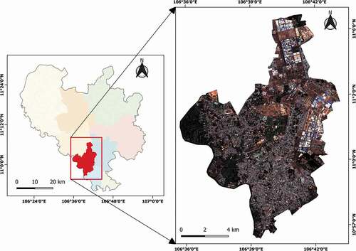
Thu Dau Mot City is the administrative, economic, and cultural center of Binh Duong province, Vietnam. The city is located in the southwest of the province, between 10°56′22″ to 11°06′41″ N latitude and 106°35′42″ to 106°44′00″ E longitude (Figure 1). It belongs to the tropical monsoon climate, which has the rainy season from May to November and the dry season from December to April of the following year. Its annual mean temperature is 27.8°C; its annual rainfall ranges from 2104 mm to 2484 mm; and its annual mean air humidity varies from 70 to 96% (Binh Duong Statistical Office 2019). The mean elevation of the city is from 6 to 40 m, and it increases from west to east and from south to north. However, the terrain surface is relatively flat, and the majority of the city has a slope of 7 degrees or less. The total area of the city is about 118.91 km², and its population was 306,564 in 2018 (Binh Duong Statistical Office 2019).

Figure 1. Study area.

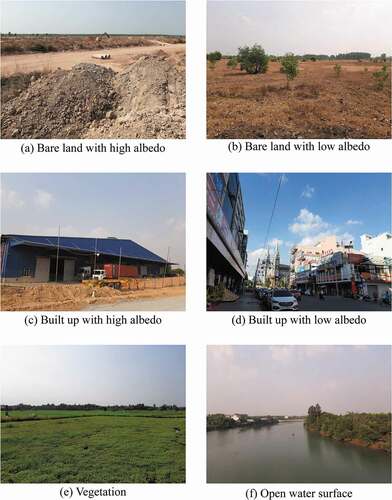
The main types of land cover in the city are built up, vegetation, bare land, and water surface. Based on a field survey trip in January 2020 and careful consideration of the characteristics of each land cover subject, the land cover in the study area was categorized into the following classes (Figure 2):

1. Bare land with high albedo (BL_H): including totally bare soil areas without any cover or very little vegetation.

2. Bare land with low albedo (BL_L): including bare land areas partly covered with sunburned vegetation and/or little fresh vegetation.

3. Built-up with high albedo (BU_H): mainly including factories and industrial buildings that are often light-colored corrugated iron or concrete.

4. Built-up with low albedo (BU_L): mainly including residences, commercial and office buildings, and roads that are often concrete, clay, tole, asphalt, or a mix of these materials.

5. Vegetation (VE): including crops, fruit trees, industrial trees, mature trees for landscaping, and fresh grass.

6. Open water surface (WA): including rivers, canals, lakes, ponds, and pools.

Figure 2. Land cover classes in the study area.

3. Materials and methods

3.1. Data

3.1.1. Satellite images

One free-cloud tile of S-2A Multispectral Instrument (MSI) Level-2A and one tile of S-1A Ground Range Detected (GRD), which cover the study area, were downloaded from the Copernicus Scientific Data Hub (https://scihub.copernicus.eu/).

The S-2A MSI Level-2A product provides the bottom of atmosphere (BOA) reflectance images. The product includes four bands of 10 m (2, 3, 4, 8), six bands of 20 m (5, 6, 7, 8A, 11, 12), and two bands of 60 m (1, 9). The cirrus band 10 was omitted as it does not contain surface information. The product’s band wavelength ranges from about 493 nm to 2190 nm, and its radiometric resolution is 12 bits.

The S-1A GRD product provides the C-band SAR data, which had been detected, multi-looked and projected to ground range using an Earth ellipsoid model. The acquired imagery was collected in the Interferometric Wide Swath (IW) mode with high resolution (a pixel spacing of 10 m and a spatial resolution of approximately 20 m × 22 m) in dual-polarization mode: vertical transmit-vertical receive (VV) and vertical transmit-horizontal receive (VH).

Due to its climatic characteristics, the study area is often covered by clouds during the rainy season (i.e. from May to November). Therefore, in this study, the optical product was collected in the dry season. One free-cloud tile of S-2, acquired on 22 February 2020 was selected. Meanwhile, although the radar product is not affected by cloud coverage, the selected tile of S-1 was acquired on 25 February 2020 to minimize the change in the land cover.

3.1.2. Vector data

The administrative boundary of the study area was downloaded from the Database of Global Administrative Areas (GADM) project website (https://gadm.org/). It was used for subsetting and masking the satellite images.

The training dataset for the six land cover classes was collected based on the results of the field trip in January 2020 combined with Google Earth images. The validation data were collected based on a stratified random sampling strategy. Based on the classification result of the S-2 dataset, the proportion of each land cover class was roughly estimated by visual observation. Based on the proportion, 70 points of BL_H, 150 points of BL_L, 90 points of BU_H, 150 points of BU_L, 140 points of VE, and 50 points of WA were randomly selected. Thus, a total of 650 points were generated. These points were visually interpreted by the S-2 image, Google Earth image, and the authors’ personal knowledge. Some points being on mixed pixels, which could not be interpreted correctly, were discarded. As a result, only 532 points could be used for validation, including 56 points of BL_H, 86 points of BL_L, 89 points of BU_H, 135 points of BU_L, 115 points of VE, and 51 points of WA.

3.2. Methods

Five main steps were carried out to achieve the study goals. First, the downloaded S-1 and S-2 data were pre-processed, and their textures and indices were extracted. In the second step, the products obtained were stacked into different datasets, including the datasets from single sensors and the fused datasets from multiple sensors. The datasets were categorized into two groups based on whether they included textures and indices or not. In the third step, the RF classifier was then applied to each dataset, and the accuracy of their results was assessed. In the fourth step, the classification results of the single-sensor datasets within each group were used as the inputs for the decision-level fusion based on D-S theory. Finally, the accuracy of classification results at the decision level was assessed and compared to those at the pixel level. The overall process followed in this study is presented in Figure 3 and described in detail below.

Figure 3. Process flowchart.

3.2.1. Pre-processing and extracting indices and textures

The S-2 tile was downloaded as a Level 2 product in WGS 84/UTM Zone 48 N projection, which has already applied geometric and atmospheric correction and is ready to use for classification. Bands 2, 3, 4, 8 (10 m) 5, 6, 7, 8A, 11, 12 (20 m) were used in this study. The 20-m bands were resampled to the 10-m ones using the nearest neighbor method to ensure the preservation of original values. Then, the Normalized Difference Vegetation Index (NDVI) and Normalized Difference Water Index (NDWI) were extracted. These two indices were included in this study because they have been widely used and have shown the potential to improve land cover classification results (Shao et al. 2016; Tian et al. 2016).

Several common pre-processing steps were applied with the downloaded S-1 GRD tile. They included apply orbit file, thermal noise removal, calibration, speckle filtering, range-Doppler terrain correction using WGS 84/UTM Zone 48 N projection and 30 m Shuttle Radar Topography Mission (SRTM), and conversion to dB (sigma0 dB) for both VH and VV. The pre-processed products had a resolution of 10 m. Speckle filtering was used for reducing noise to improve image quality (Filipponi 2019); however, it also can lead to a massive loss of information when extracting texture features (Hu, Ghamisi, and Zhu 2018). Therefore, there were two sets of products in this step: VH and VV with speckle filtering were used as input data for classifiers, and the ones without speckle filtering were used for extracting textures. Afterward, eight gray-level co-occurrence matrix (GLCM) textures were derived for both VH and VV by using a 9 × 9 window size in all directions. The derived textures included mean, correlation, variance, homogeneity, contrast, dissimilarity, entropy, and angular second moment. As a result, 16 texture products were generated.

Because there was a small shift in pixels between the optical and SAR products, the resulting products were aligned using band 2 of S-2 as a reference image to make them fit together. Finally, all products were subset to the study area. These pre-processing steps were conducted on the Sentinel Application Platform (SNAP) and Quantum Geographic Information System (QGIS) software.

3.2.2. Combination, classification, and accuracy assessment

After pre-processing, the products were stacked into different datasets, including the datasets from single sensors (D1, D2, D3, and D4) and the fused datasets from multiple sensors (D5 and D6). This study applied the common combination method of layer stacking to fuse the data from S-1 and S-2 together at the pixel level. The datasets were then categorized into two groups: a group of datasets containing only spectral and backscattering bands (group 1) and a group of datasets consisting of these bands and their extracted textures and indices (group 2). Table 1 summarizes the information of all datasets.

Table 1. Summary of the input datasets.

Dataset	Data sources	Variables	Note
D1	S-1 only	VH, VV	Group 1
D2	S-2 only	2, 3, 4, 5, 6, 7, 8, 8A, 11, 12	Group 1
D3	S-1 with GLCM textures	VH, VV, and textures of mean, correlation, variance, homogeneity, contrast, dissimilarity, entropy, and angular second moment of VH and VV	Group 2
D4	S-2 with indices	2, 3, 4, 5, 6, 7, 8, 8A, 11, 12, NDVI, NDWI	Group 2
D5	D1 and D2	All variables of D1 and D2	Group 1, pixel-level fusion
D6	D3 and D4	All variables of D3 and D4	Group 2, pixel-level fusion
D7	Random forest results of D1 and D2	Probability of each land cover class, and OA, or UA, or PA of each result	Group 1, decision-level fusion
D8	Random forest results of D3 and D4	Probability of each land cover class, and OA, or UA, or PA of each result	Group 2, decision-level fusion

GLCM = gray-level co-occurrence matrix; VV = vertical transmit-vertical receive; VH = vertical transmit-horizontal receive; NDVI = Normalized Difference Vegetation Index; NDWI = Normalized Difference Water Index; OA = overall accuracy; UA = user’s accuracy; PA = producer’s accuracy.

In this study, the RF algorithm, developed by Breiman (2001), was selected as the classifier for land cover classification at the pixel level. A random forest consists of a set of decision trees, each of which is generated by randomly drawing a subset from the training dataset. From the results of the trees, a majority vote is conducted to determine the final output (Xie et al. 2019). RF is easy to use, highly efficient, fast to process, and suitable for remote sensing applications (Belgiu and Drăguţ 2016; Gudmann et al. 2020). Since its results come from voting, RF has the ability to produce classification output as probabilities of each class, which was used as the input for fusion at the decision level. The classification process was implemented on R software, using the “randomForest” package (Liaw and Wiener 2002). Two important parameters affecting the classification performance of the RF model are the maximum number of trees (ntree) and the number of variables randomly sampled as candidates at each split (mtry). The mtry parameter was set at the default value, which is equal to the square root of the total number of features. After testing the relationship between the ntree and the decrease in out-of-bag error rates, the ntree was set at 300 trees as out-of-bag error rates were relatively stable after this point. The composited datasets were used as inputs for the classification process. As a result, six land cover maps were generated at the pixel level, and their accuracy was then assessed. In addition, four classification results of single-sensor datasets, in the form of probabilities of each land cover class, were also produced to use in the next stages.

At the decision level, the probability-form classification results were fused within each group. The classification result of D1 was fused with that of D2 (D7), while the results of D3 and D4 were combined (D8). This study applied the data fusion method based on the D-S evidence theory (Dempster 1967; Shafer 1976) using the dst package (Boivin and Stat. ASSQ 2020) in R software. D-S evidence theory, which is often described as a generalization of the Bayesian theory, is based on belief functions and plausible reasoning. The advantages the theory offer in data classification include: (i) flexible construction of the mass function and the data organization; (ii) no requirement regarding the prior knowledge or conditional probabilities, which makes it suitable for handling data with unseen labels; and (iii) possibility to provide the uncertainty of the result (Chen et al. 2014). Theoretical calculation steps were carried out according to the detailed description of Shao et al. (2016). The Basic Probability Assignment (BPA – or mass function) of each pixel, which is a prerequisite for fusion according to D-S theory, was calculated as follows:

$m_i\left(A\right)=p_v\times p_i$

in which m_i (A) is the mass function value of the calculated pixel in class A of data source i, p_v is the probability of belonging to each land cover class of the calculated pixel, and p_i is the probability of correct classification of data source i. In this study, the OA, user’s accuracy (UA) and producer’s accuracy (PA) were used in turn to measure the probability of correct classification for the calculation.

As a result, six land cover maps (two by using OA, two by using UA, and two by using PA) were generated at this decision level, and their accuracy was then assessed. Finally, the accuracy of all classification results at both pixel and decision levels was compared by both visual assessment and OA, PA, UA, and Kappa coefficients.

4. Results and discussion

The accuracy assessments of all classification results are presented in Table 2. The land cover maps of the two groups are also presented in Figures 4 and 5. The fusion results using PA were chosen as a representation of the decision level in these figures.

Table 2. Comparison of the overall accuracy and Kappa coefficient of the classification result of all datasets.

Dataset	Overall Accuracy (%)	Kappa coefficient
Group 1: datasets without textures and indices
D7 using OA	90.60	0.88
D7 using PA	90.23	0.88
D7 using UA	90.23	0.88
D2	89.47	0.87
D5	84.59	0.81
D1	42.86	0.29
Group 2: datasets with textures and indices
D8 using UA	92.67	0.91
D8 using PA	91.92	0.90
D8 using OA	91.35	0.89
D4	90.60	0.88
D6	84.02	0.80
D3	52.07	0.41

OA = overall accuracy; UA = user’s accuracy; PA = producer’s accuracy.

Figure 4. Land cover maps from the datasets without textures and indices: (a) dataset D1; (b) dataset D2; (c) dataset D5; (d) dataset D7 using PA.

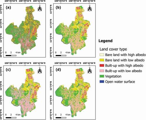
Figure 5. Land cover maps from the datasets with textures and indices: (a) dataset D3; (b) dataset D4; (c) dataset D6; (d) dataset D8 using PA.

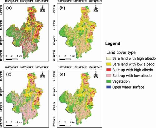
In group 1, the fusion method using D-S theory provided the most accurate results, in which OA ranged from 90.23% to 90.60% and the Kappa coefficient was 0.88. The best result in this group occurred in the fusion of D7, based on the OA. Similarly, results from the decision-level fusion in group 2 also gave the highest accuracy, with the OA ranging from 91.35% to 92.67% and the Kappa coefficient varying from 0.89 to 0.91. The fusion of D8 using UA produced the best result in this group with an OA of 92.67% and a Kappa coefficient of 0.91. It was also the product with the most accuracy in all datasets. Therefore, the highest accuracy was found in the results of fusion at the decision level in both groups, whether using OA, UA, or PA for mass function construction. In contrast, the poorest results occurred in S-1 only (OA = 42.86%, Kappa = 0.29) in group 1 and in S-1 with its texture variables (OA = 52.07%, Kappa = 0.41) in group 2. In general, both groups followed a similar trend in the accuracy of mapping results from datasets and decreased in the following order: decision-level fusion dataset, single optical dataset, pixel-level fusion dataset, and single SAR dataset.

As a result, the fusion results from S-1 and S-2 products at the decision level increased mapping accuracy by a range of 0.75% to 2.07% in comparison to the results of corresponding S-2 products in the two groups. D-S theory considered each land cover class from different inputs as independent evidence. Evidential probability was constructed entirely based on the results of the classification algorithm at the pixel level, without taking into account the input of that algorithm. Therefore, this evidence theory could reduce the impact of noise data and feature selection in land cover classification (Shao et al. 2016). By that advantage, the use of D-S theory at the decision level in this study produced mapping results with a higher level of accuracy. This finding is consistent with many previous studies (Ran et al. 2012; Shao et al. 2016; Mezaal, Pradhan, and Rizeei 2018). It is clear that the result of the D-S fusion depends on how the mass function is constructed. Mezaal, Pradhan, and Rizeei (2018) converted the posterior probabilities of the classification results to the form of mass function directly; Ran et al. (2012) identified the parameter for the mass function construction from a literature review and expert knowledge; The p_v parameter of the mass function in Shao et al. (2016) was similar to our study, and the p_i was based on the PA of each class. This study is distinguished by testing the construction of mass function using the OA, UA, and PA in turn for the parameter of p_i to get a more comprehensive assessment of the effectiveness of the D-S theory-based fusion. As mentioned, each of the three construction methods yielded better results than that of single-sensor and fused datasets at the pixel level. The results show that whether using the OA, UA, or PA for mass function construction, applying the D-S fusion method on S-1 and S-2 data provides a better result for land cover mapping. In addition, the results suggest that such a method is applicable for high-accuracy mapping in other urban areas.

However, the fusion data from different sensors using the layer-stacking technique at the pixel level did not improve classification efficiency. It reduced the accuracy of classification by a range of 4.88% to 6.58% compared to the results of corresponding optical products in the two groups. Although most studies in the literature reported the ability to improve the overall accuracy when fusing various data sources at the pixel level compared to using a single data source, some studies have shown the opposite (de Furtado et al. 2015; Fonteh et al. 2016). Zhang and Xu (2018) found that whether the combination of optical and SAR data could improve the accuracy of urban land cover mapping or not depended on the fusion levels and the fusion methods. Therefore, in our study, the extraction and selection of variables as well as the choice of combination technique and classification algorithm may have influenced the outcome of the classification. To improve mapping performance at the pixel level, further studies are needed to determine the optimal variable selection for data integration and to test other fusion techniques, such as the component substitution methods or the multi-scale decomposition methods (Kulkarni and Rege 2020).

When comparing the results from group 1 and group 2, the accuracy of most of the datasets containing indices and textures was higher than that of the corresponding datasets without these extracted variables, except for the pair of datasets D5 and D6. The most significant increase took place in the pair of datasets D1 and D3, where the addition of the GLCM textures along with VH and VV raised the OA by 9.21%. The accuracy of the remaining pairs also increased by a range of 1.12% to 2.07% when including these extracted variables in the datasets. This finding confirms that the GLCM textures can provide additional useful information to improve classification results (Lu et al. 2014; Zakeri, Yamazaki, and Liu 2017; Tavares et al. 2019); however, the effectiveness of spectral indices is still controversial. Our results showed the spectral indices were effective in land cover classification to some extent. While many studies have included some common spectral indices (e.g. NDVI, NDWI, and Normalized Difference Built-up Index) in the input dataset and enhanced the accuracy of mapping results (Shao et al. 2016; Tian et al. 2016; Abdi 2020), other studies have indicated the opposite results (Adepoju and Adelabu 2020; Tavares et al. 2019). This discrepancy may result from differences in land cover characteristics of the study areas and the selection of indices included in the dataset. Therefore, these indices should be used with caution in future studies.

A detailed comparison of PA and UA in each class of each classification result is presented in Tables 3 and 4. In addition, three example regions from classification maps in group 2 are presented in Figure 6 to provide a visual comparison. The Google Earth images were captured on 16 April 2020 using the historical imagery function on Google Earth Pro software. As seen in Tables 3 and 4

Table 3. The producer’s accuracy and user’s accuracy of the classification result of the datasets without textures and indices.

Dataset	Accuracy index	Class
		BL_H	BL_L	BU_H	BU_L	VE	WA
D1	PA (%)	10.71	46.51	41.57	43.70	64.35	23.53
	UA (%)	60.00	31.50	37.37	51.30	49.01	40.00
D2	PA (%)	91.07	93.02	87.64	83.70	91.30	96.08
	UA (%)	89.47	73.39	92.86	91.13	97.22	98.00
D5	PA (%)	92.86	61.63	92.13	86.67	86.96	90.20
	UA (%)	94.55	69.74	95.35	71.34	97.09	95.83
D7 using OA	PA (%)	91.07	94.19	86.52	88.15	92.17	94.12
	UA (%)	89.47	78.64	95.06	89.47	97.25	97.96
D7 using UA	PA (%)	91.07	88.37	86.52	89.63	92.17	96.08
	UA (%)	89.47	83.52	92.77	86.43	96.36	96.08
D7 using PA	PA (%)	91.07	95.35	86.52	85.93	92.17	94.12
	UA (%)	89.47	77.36	95.06	89.92	96.36	97.96

BL_H = Bare land with high albedo; BL_L = Bare land with low albedo; BU_H = Built-up with high albedo; BU_L = Built-up with low albedo; VE = Vegetation; WA = Open water surface; OA = overall accuracy; UA = user’s accuracy; PA = producer’s accuracy.

Table 4. The producer’s accuracy and user’s accuracy of the classification result of the datasets with textures and indices.

Dataset	Accuracy index	Class
		BL_H	BL_L	BU_H	BU_L	VE	WA
D3	PA (%)	7.14	47.67	78.65	45.93	60.00	60.78
	UA (%)	50.00	44.57	46.67	50.82	58.47	73.81
D4	PA (%)	96.43	91.86	92.13	83.70	95.65	86.27
	UA (%)	94.74	73.83	94.25	91.87	96.49	100.00
D6	PA (%)	83.93	63.95	91.01	87.41	87.83	88.24
	UA (%)	95.92	74.32	88.04	69.82	98.06	100.00
D8 using OA	PA (%)	91.07	90.70	95.51	87.41	95.65	86.27
	UA (%)	98.08	75.00	97.70	90.77	95.65	100.00
D8 using UA	PA (%)	94.64	87.21	95.51	91.11	94.78	94.12
	UA (%)	98.15	83.33	98.84	89.13	95.61	96.00
D8 using PA	PA (%)	92.86	91.86	95.51	86.67	95.65	90.20
	UA (%)	98.11	75.96	97.70	92.13	95.65	100.00

, while S-1 only and S-1 with GLCM texture classification results yielded relatively low accuracy, the majority of PA and UA of all classes from other classifications were high (over 85%). BL_L was the class that had the most misclassifications, which resulted in the lowest accuracy in most cases.

Figure 6. Comparison of the classification results from the datasets with textures and indices in three example regions.

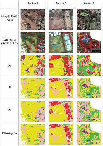
At the pixel level, the fusion data from different sources significantly reduced the PA of BL_L and the UA of BU_L when compared to the corresponding S-2 products in both fusion cases. The former was reduced by 31.39% in the datasets without derived products and by 27.91% in the datasets with derived products. Meanwhile, the latter was decreased by 19.79% in the datasets of group 1 and by 22.05% in the datasets of group 2. The misclassification between these two classes could be clearly seen in the three sample regions, in which the BU_L areas, especially roads, were misclassified as bare land. Moreover, with the BU_H class, the misclassification from bare land areas to factories and from factories to low albedo built-up areas decreased, but the misclassification between factories and totally bare soil areas increased. Therefore, the UA and PA of classes increased or decreased unevenly, but overall, the total reduction was greater than the total increase in both fusion cases.

On the contrary, at the decision level, although the UA and PA of classes also increased or decreased unevenly, the total reduction was lower than the total increase in both fusion cases. By visual assessment, the greatest improvement was found in the classes BU_H, BU_L, and BL_L. In these classes, the misclassification from high-albedo build-up to bare soil and to low-albedo built-up was significantly reduced, contributing to the increase in the OA of the mapping result. However, because the BU_H class only took a small proportion of the study area (about 5% of the total area), the reduced misclassification only resulted in a slight increase in the OA compared to the maps from the optical datasets.

In general, in most cases of both single-sensor datasets and integrated datasets, the BU_L and BL_L had the highest rate of misclassification among all classes, which may be due to the similarity in their spectral characteristics. The study results of Chen et al. (2019), Li et al. (2017), Shao et al. (2016), and Wei et al. (2020) and many others have also shown this issue. Meanwhile, although the UA of water class achieved up to 100%, some water areas were misclassified as high albedo built-up area by visual assessment in all datasets at the nearshore of an artificial swimming pool in example region 3. The misclassification from WA to BU_H in this region may be explained by a few factors. First, the pool is in the Dai Nam Wonderland water park, and in fact, it is an artificial sea with saline water, not a freshwater swimming pool. The depth of this artificial sea gradually rises from the nearshore to the offshore, where the shallower water leads to higher reflectance contribution from the floor material of the water area (Chuvieco and Huete 2016); Second, the floor of this artificial sea is made of light-colored concrete, which belongs to BU_H class. These factors combined may have caused the misclassification from water to high-albedo built-up area at the nearshore area of the sea. For the vegetation class, the difference in the accuracy was not significant between the fused datasets and corresponding optical datasets.

5. Conclusions

In summary, the fusion of S-1 and S-2 data based on D-S theory at the decision level yielded better mapping results compared to others. It comes from the advantages of the D-S theory-based technique in reducing the impact of noise data and feature selection in land cover classification. The most obvious improvement was found in the classes of barren land and built up. As a result, the datasets fused at the decision level increased the OA by a range of 0.75% to 2.07% compared to the S-2 datasets. The fusion of S-1 and S-2 data with their derived textures and indices at the decision level using D-S theory brought the best results in this study, achieving an OA and Kappa coefficient of 92.67% and 0.91, respectively.

Moreover, the integration of SAR and optical products using the layer-stacking technique at the pixel level did not give more power to the classification process. It reduced the accuracy of the mapping result by 4.88% to 6.58% compared to that of the optical datasets. These findings may be influenced by the processing and selection of features, fusion technique, and classifier. Further studies on this issue are needed.

Furthermore, the inclusion of GLCM textures and spectral indices in the datasets helped improve the mapping results. However, while the effectiveness of the textures is clear, the contribution of the indices needs to be studied further.

In general, the results of this study show that using the D-S fusion method for high-accuracy mapping in other urbanized areas holds great potential. This study represents an initial step, and it paves the way for further research on land cover mapping using additional available data from the active and passive sensors for performance improvement.

Acknowledgments

The authors would like to thank Mr. Claude Boivin, who is the author of the “dst” package, for his detailed instructions in using this package. The authors also would like to thank the editors and reviewers for their helpful comments and suggestions.

Data availability statement

The satellite images can be downloaded from the Copernicus Scientific Data Hub (https://scihub.copernicus.eu/). The administrative boundary can be downloaded from the Database of Global Administrative Areas project website (https://gadm.org/). The ground truth data and R code are available from the corresponding author, [Dang Hung Bui], upon reasonable request.

Disclosure statement

No potential conflict of interest was reported by the author(s).

Additional information

Funding

This work is supported by the Hungarian Scientific Research Fund in support of the ongoing research, “Time series analysis of land cover dynamics using medium- and high-resolution satellite images” [grant number NKFIH 124648K], at the Department of Physical Geography and Geoinformatics (the former name of the Department of Geoinformatics, Physical and Environmental Geography), University of Szeged, Szeged, Hungary.

Notes on contributors

Dang Hung Bui

Dang Hung Bui received his master’s degree in environmental management from the Ho Chi Minh City University of Technology, Vietnam National University Ho Chi Minh City, Vietnam in 2014. He is currently pursuing a PhD’s degree at the Doctoral School of Geosciences, University of Szeged, Hungary. His research interests are land use land cover monitoring and classification by using remote sensing and geographic information systems.

László Mucsi

László Mucsi is an associate professor at the Department of Geoinformatics, Physical and Environmental Geography, University of Szeged, Hungary. His research interests are the applications of advanced techniques of remote sensing and geographic information systems in land use mapping, urban remote sensing, and impervious surface detection.

References

- Abdi, A.M. 2020. “Land Cover and Land Use Classification Performance of Machine Learning Algorithms in a Boreal Landscape Using Sentinel-2 Data.” GIScience and Remote Sensing 57 (1): 1–20. doi:10.1080/15481603.2019.1650447.
- Adepoju, K.A., and S.A. Adelabu. 2020. “Improving Accuracy of Landsat-8 OLI Classification Using Image Composite and Multisource Data with Google Earth Engine.” Remote Sensing Letters 11 (2): 107–116. doi:10.1080/2150704X.2019.1690792.
- Arowolo, A.O., X. Deng, O.A. Olatunji, and A.E. Obayelu. 2018. “Assessing Changes in the Value of Ecosystem Services in Response to Land-Use/Land-Cover Dynamics in Nigeria.” Science of the Total Environment 636: 597–609. doi:10.1016/j.scitotenv.2018.04.277.
- Ban, Y., H. Hu, and I.M. Rangel. 2010. “Fusion of Quickbird MS and RADARSAT SAR Data for Urban Land-Cover Mapping: Object-Based and Knowledge-Based Approach.” International Journal of Remote Sensing 31 (6): 1391–1410. doi:10.1080/01431160903475415.
- Belgiu, M., and L. Drăguţ. 2016. “Random Forest in Remote Sensing: A Review of Applications and Future Directions.” ISPRS Journal of Photogrammetry and Remote Sensing 114: 24–31. doi:10.1016/j.isprsjprs.2016.01.011.
- Binh Duong Statistical Office. 2019. Statistical Yearbook of Binh Duong 2018. Vietnam: Binh Duong.
- Boivin, C., and Stat. ASSQ. 2020. “Dst: Using the Theory of Belief Functions.” https://cran.r-project.org/package=dst
- Breiman, L. 2001. “Random Forests.” Machine Learning 45 (1): 5–32. doi:10.1023/A:1010933404324.
- Cai, G., H. Ren, L. Yang, N. Zhang, M. Du, and C. Wu. 2019. “Detailed Urban Land Use Land Cover Classification at the Metropolitan Scale Using a Three-Layer Classification Scheme.” Sensors 19 (14): 3120. doi:10.3390/s19143120.
- Chen, Y., W. Huang, W.H. Wang, J.Y. Juang, J.S. Hong, T. Kato, and S. Luyssaert. 2019. “Reconstructing Taiwan’s Land Cover Changes between 1904 and 2015 from Historical Maps and Satellite Images.” Scientific Reports 9: 3643. doi:10.1038/s41598-019-40063-1.
- Chen, Q., A. Whitbrook, U. Aickelin, and C. Roadknight. 2014. “Data Classification Using the Dempster-Shafer Method.” Journal of Experimental and Theoretical Artificial Intelligence 26 (4): 493–517. doi:10.1080/0952813X.2014.886301.
- Chuvieco, E., and A. Huete. 2016. Fundamentals of Satellite Remote Sensing: An Environmental Approach. Boca Raton, FL: CRC Press.
- de Furtado, L.F.A., T.S.F. Silva, P.J.F. Fernandes, and E.M.L. de Moraes de Novo. 2015. “Land Cover Classification of Lago Grande de Curuai Floodplain (Amazon, Brazil) Using Multi-Sensor and Image Fusion Techniques.” Acta Amazonica 45 (2): 195–202. doi:10.1590/1809-4392201401439.
- Dempster, A.P. 1967. “Upper and Lower Probabilities Induced by a Multivalued Mapping.” Annals of Mathematical Statistics 38 (2): 325–339. doi:10.1214/AOMS/1177698950.
- Filipponi, F. 2019. “Sentinel-1 GRD Preprocessing Workflow.” Proceedings 18 (1): 11. doi:10.3390/ecrs-3-06201.
- Fonteh, M.L., F. Theophile, M.L. Cornelius, R. Main, A. Ramoelo, and M.A. Cho. 2016. “Assessing the Utility of Sentinel-1 C Band Synthetic Aperture Radar Imagery for Land Use Land Cover Classification in a Tropical Coastal Systems When Compared with Landsat 8.” Journal of Geographic Information System 8 (4): 495–505. doi:10.4236/jgis.2016.84041.
- Grigoraș, G., and B. Urițescu. 2019. “Land Use/Land Cover Changes Dynamics and Their Effects on Surface Urban Heat Island in Bucharest, Romania.” International Journal of Applied Earth Observation and Geoinformation 80: 115–126. doi:10.1016/j.jag.2019.03.009.
- Guan, X., S. Liao, J. Bai, F. Wang, Z. Li, Q. Wen, J. He, and T. Chen. 2017. “Urban Land-Use Classification by Combining High-Resolution Optical and Long-Wave Infrared Images.” Geo-spatial Information Science 20 (4): 299–308. doi:10.1080/10095020.2017.1403731.
- Gudmann, A., N. Csikós, P. Szilassi, and L. Mucsi. 2020. “Improvement in Satellite Image-Based Land Cover Classification with Landscape Metrics.” Remote Sensing 12 (21): 3580. doi:10.3390/rs12213580.
- Hall, D.L., and J. Llinas. 1997. “An Introduction to Multisensor Data Fusion.” Proceedings of the IEEE 85 (1): 6–23. doi:10.1109/5.554205.
- Hu, J., P. Ghamisi, and X. Zhu. 2018. “Feature Extraction and Selection of Sentinel-1 Dual-Pol Data for Global-Scale Local Climate Zone Classification.” ISPRS International Journal of Geo-Information 7 (9): 379. doi:10.3390/ijgi7090379.
- Kulkarni, S.C., and P.P. Rege. 2020. “Pixel Level Fusion Techniques for SAR and Optical Images: A Review.” Information Fusion 59: 13–29. doi:10.1016/j.inffus.2020.01.003.
- Li, H., C. Wang, C. Zhong, A. Su, C. Xiong, J. Wang, and J. Liu. 2017. “Mapping Urban Bare Land Automatically from Landsat Imagery with a Simple Index.” Remote Sensing 9 (3): 249. doi:10.3390/rs9030249.
- Liaw, A., and M. Wiener. 2002. “Classification and Regression by RandomForest.” R News 2 (3): 18–22. https://cran.r-project.org/doc/Rnews/
- Liu, Y., W. Gong, X. Hu, and J. Gong. 2018. “Forest Type Identification with Random Forest Using Sentinel-1A, Sentinel-2A, Multi-Temporal Landsat-8 and DEM Data.” Remote Sensing 10 (6): 946. doi:10.3390/rs10060946.
- Lu, D., G. Li, E. Moran, L. Dutra, and M. Batistella. 2014. “The Roles of Textural Images in Improving Land-Cover Classification in the Brazilian Amazon.” International Journal of Remote Sensing 35 (24): 8188–8207. doi:10.1080/01431161.2014.980920.
- Lu, D., and Q. Weng. 2007. “A Survey of Image Classification Methods and Techniques for Improving Classification Performance.” International Journal of Remote Sensing 28 (5): 823–870. doi:10.1080/01431160600746456.
- Mezaal, M.R., B. Pradhan, and H.M. Rizeei. 2018. “Improving Landslide Detection from Airborne Laser Scanning Data Using Optimized Dempster-Shafer.” Remote Sensing 10 (7): 1029. doi:10.3390/rs10071029.
- Mfuka, C., E. Byamukama, and X. Zhang. 2020. “Spatiotemporal Characteristics of White Mold and Impacts on Yield in Soybean Fields in South Dakota.” Geo-spatial Information Science 23 (2): 182–193. doi:10.1080/10095020.2020.1712265.
- Pohl, C., and J. van Genderen. 2016. Remote Sensing Image Fusion: A Practical Guide. London: CRC Press.
- Prins, A.J., and A. Van Niekerk. 2020. “Crop Type Mapping Using LiDAR, Sentinel-2 and Aerial Imagery with Machine Learning Algorithms.” Geo-spatial Information Science 24 (2): 1–13. doi:10.1080/10095020.2020.1782776.
- Ran, Y.H., X. Li, L. Lu, and Z.Y. Li. 2012. “Large-Scale Land Cover Mapping with the Integration of Multi-Source Information Based on the Dempster-Shafer Theory.” International Journal of Geographical Information Science 26 (1): 169–191. doi:10.1080/13658816.2011.577745.
- Rimal, B., L. Zhang, H. Keshtkar, N. Wang, and Y. Lin. 2017. “Monitoring and Modeling of Spatiotemporal Urban Expansion and Land-Use/Land-Cover Change Using Integrated Markov Chain Cellular Automata Model.” ISPRS International Journal of Geo-Information 6 (9): 288. doi:10.3390/ijgi6090288.
- Schmitt, M., and X. Zhu. 2016. “Data Fusion and Remote Sensing: An Ever-Growing Relationship.” IEEE Geoscience and Remote Sensing Magazine 4 (4): 6–23. doi:10.1109/MGRS.2016.2561021.
- Shafer, G. 1976. A Mathematical Theory of Evidence. Princeton: Princeton University Press.
- Shao, Z., G. Cheng, D. Li, X. Huang, Z. Lu, and J. Liu. 2021a. “Spatio-Temporal-Spectral-Angular Observation Model that Integrates Observations from UAV and Mobile Mapping Vehicle for Better Urban Mapping.” Geo-spatial Information Science 24 (4): 615–629. doi:10.1080/10095020.2021.1961567.
- Shao, Z., H. Fu, P. Fu, and L. Yin. 2016. “Mapping Urban Impervious Surface by Fusing Optical and SAR Data at the Decision Level.” Remote Sensing 8 (11): 945. doi:10.3390/rs8110945.
- Shao, Z., N.S. Sumari, A. Portnov, F. Ujoh, W. Musakwa, and P.J. Mandela. 2021b. “Urban Sprawl and Its Impact on Sustainable Urban Development: A Combination of Remote Sensing and Social Media Data.” Geo-spatial Information Science 24 (2): 241–255. doi:10.1080/10095020.2020.1787800.
- Solberg, A.H.S. 2006. “Data Fusion for Remote Sensing Applications.” In Signal and Image Processing for Remote Sensing, edited by C. H. Chen, 515–537. Boca Raton, FL: CRC Press.
- Tabib Mahmoudi, F., A. Arabsaeedi, and S.K. Alavipanah. 2019. “Feature-Level Fusion of Landsat 8 Data and SAR Texture Images for Urban Land Cover Classification.” Journal of the Indian Society of Remote Sensing 47 (3): 479–485. doi:10.1007/s12524-018-0914-8.
- Tavares, P.A., N.E. Santos Beltrão, U.S. Guimarães, and A.C. Teodoro. 2019. “Integration of Sentinel-1 and Sentinel-2 for Classification and LULC Mapping in the Urban Area of Belém, Eastern Brazilian Amazon.” Sensors 19 (5): 1140. doi:10.3390/s19051140.
- The European Space Agency. 2021. “Sentinel Overview.” https://sentinel.esa.int/web/sentinel/missions
- Tian, S., X. Zhang, J. Tian, and Q. Sun. 2016. “Random Forest Classification of Wetland Landcovers from Multi-Sensor Data in the Arid Region of Xinjiang, China.” Remote Sensing 8 (11): 954: 1–14. doi:10.3390/rs8110954.
- Wei, B., Y. Xie, X. Wang, J. Jiao, S. He, Q. Bie, X. Jia, X. Xue, and H. Duan. 2020. “Land Cover Mapping Based on Time Series MODIS NDVI Using A Dynamic Time Warping Approach: A Casestudy of the Agricultural Pastoral Ecotone of Northern China.” Land Degradation & Development 31 (8): 1050–1068. doi:10.1002/ldr.3502.
- Xie, Z., Y. Chen, D. Lu, G. Li, and E. Chen. 2019. “Classification of Land Cover, Forest, and Tree Species Classes with Ziyuan-3 Multispectral and Stereo Data.” Remote Sensing 11 (2): 164. doi:10.3390/rs11020164.
- Xu, L., and A. Ma. 2021. “Coarse-to-Fine Waterlogging Probability Assessment Based on Remote Sensing Image and Social Media Data.” Geo-spatial Information Science 24 (2): 279–301. doi:10.1080/10095020.2020.1812445.
- Zakeri, H., F. Yamazaki, and W. Liu. 2017. “Texture Analysis and Land Cover Classification of Tehran Using Polarimetric Synthetic Aperture Radar Imagery.” Applied Sciences 7 (5): 452. doi:10.3390/app7050452.
- Zhang, J. 2010. “Multi-Source Remote Sensing Data Fusion: Status and Trends.” International Journal of Image and Data Fusion 1 (1): 5–24. doi:10.1080/19479830903561035.
- Zhang, H., and R. Xu. 2018. “Exploring the Optimal Integration Levels between SAR and Optical Data for Better Urban Land Cover Mapping in the Pearl River Delta.” International Journal of Applied Earth Observation and Geoinformation 64: 87–95. doi:10.1016/j.jag.2017.08.013.