Evaluation and adjustment of the radiometric degradation of HY-1B satellite COCTS via a stable marine site

ABSTRACT

The Chinese Ocean Color and Temperature Scanner (COCTS) on-board the Chinese second ocean color satellite, HY-1B, obtained approximately 6 years of data between 2007 and 2013 in China coastal seas and the adjacent waters. However, its radiometric performance has hardly been analyzed, which confuses its applicability in ocean remote sensing. This study tracked the long-term radiometric responsivity trend of HY-1B COCTS based on a stable marine target. Firstly, we identified a temporally stable maritime site of 12° ~ 15°N and 116°~119°E according to the water and atmospheric optical properties using Aqua MODIS products. Then, the time-series of top-of-atmosphere (TOA) reflectance was obtained for each band of HY-1B COCTS and Aqua MODIS over this site according to the criteria of sun-target-view geometry. Finally, exponential or linear degradation models were built and used to adjust the radiometric levels of HY-1B COCTS. Results indicate that the radiometric performance exhibited continuous degradation for all bands at varying levels between 0.4% and 8.1% yr⁻¹. The worst degradation occurred at 412 nm, with an annual average rate of 8.1%. The degradation at 443 nm reached 5.5% yr⁻¹ following 412 nm. The radiometric performance at 490 nm, 520 nm, and 565 nm was relatively stable with a drift of ~3% yr⁻¹. The 670 nm, 750 nm, and 865 nm bands remain most stable with the degradation of ~1% yr⁻¹. Taking Terra MODIS as a reference, the temporal consistency of HY-1B COCTS was significantly improved for each band after radiometric adjustment. Cloud-free imageries between 2007 and 2013 showed relatively high spatial consistency. The bias of TOA reflectance was ~5% in visible bands and ~10% in near-infrared bands after degradation correction. These improvements confirm the application potentials of HY-1B COCTS in ocean remote sensing.

KEYWORDS:

• HY-1B COCTS
• radiometric degradation
• stable marine site

1. Introduction

The performance of satellite sensors degrades as a result of aging owing to the space environment, such as extreme temperature and radiation damage (Chander et al. 2010; Ioccg 2013; Ling et al. 2013). This leads to increasing calibration uncertainty and product inconsistency (Guorui, Huijie, and Hao 2014; Wang et al. 2012). Thus, it is necessary to understand the degradation processes of the instruments. For sensors with an on-board calibration system, the sensor degradation can be accurately tracked by taking advantage of a stable interior lamp, lunar or solar (Cao et al. 2014; Tsuchida et al. 2020; Xiong et al. 2007; Zhi et al. 2019). However, for other sensors without an on-board calibration system, the only reference target that can be used for recording degradation is the earth’s surface (Li et al. 2015), which is more unstable than the space target.

Typically, some studies track radiometric degradation by recording the continuous change of radiometric calibration coefficient, namely the radiometric calibration method. This method requires long-term continuous parameters of surface and atmosphere, like reflectance, aerosol optical depth, ozone concentration, and water vapor, to simulate top-of-atmosphere (TOA) radiance, then to calculate the timely calibration coefficients (Li et al. 2015; Wu 2009). In practice, to obtain these parameters, the site should be spatially homogeneous and long-term stable to reduce the uncertainty in radiative transfer simulation and its input parameters (Helder, Basnet, and Morstad 2010; Hu et al. 2020; Zibordi and Mélin 2017; Zibordi et al. 2015).

However, the optical characteristics of the earth surface, even stable site, are dynamic with illumination conditions, atmospheric environment, and the surface substance composition or geometry (Kim et al. 2014). Various Bidirectional Reflectance Distribution Function (BRDF) models and radiometric transform approaches often fail to remove the angular effects for simulating TOA radiance (Kim et al. 2014; Latifovic, Cihlar, and Jing 2003; Li et al. 2015), especially in ocean optical remote sensing practices where large view angle, bubbles, and waves often arise (Ma et al. 2015; Ruddick et al. 2014). Moreover, it is difficult to obtain long-term continuous in-situ data of water and atmosphere at relatively stable marine sites. Only a few appropriate instrumentations can provide such in-situ data, for example, MOBY located off Lanai (Clark et al. 2003) and BOUSSOLE located in the northwestern Mediterranean Sea (Antoine et al. 2008). Without in-situ measurement, these parameters can also be simulated based on other instruments’ measurements, but need to account for the different signal-noise ratios, band characteristics, spatial resolution, and transit time (Pinto et al. 2016). For these reasons, it is challenging to track the radiometric responsivity of ocean color satellite instruments based on radiometric transfer simulation.

Recent studies have shown that TOA reflectance of the target instrument over nadir overpasses can directly indicate the long-term trend of radiometric responsivity, unnecessary to calculate calibration coefficients (Chu and Wang 2020; Kim et al. 2014). It requires more rigorous sun-target-view geometry and long-term stable atmospheric properties over the earth target site (Cao 2012; Wu 2009). This kind of method can efficiently avoid uncertainty brought by radiative transfer code and simplify tracking steps.

In China, ocean color remote sensing is rapidly developing. HY-1C (Haiyang = Ocean) satellite is a follow-on mission of the HY-1A and HY-1B missions of NSOAS (National Satellite Ocean Application Service), Ministry of Natural Resources (MNR) of China. launched in 2018, can meet the requirements for providing high-quality imageries (Chen et al. 2020b; Men et al. 2022; Song et al. 2019). HY-1D was launched in 2020 as the “sister” satellite to HY-1C. The next-generation ocean color satellite is now in development (He et al. 2017) and is expected to be launched in 2022. The application of these satellites has been placed under great expectations. Except for the mentioned satellites above, the first two Chinese ocean color satellites, HY-1A and HY-1B, were launched as early as 2002 and 2007, respectively (He et al. 2008; Pan, He, and Zhu 2004). The Chinese Ocean Color and Temperature Scanner (COCTS), loaded in HY-1A/B, had obtained a large number of imageries for about 9 years. This sensor is a medium-resolution optical imager, which consists of eight visible/near-infrared bands centered at wavelength of 412, 443, 490, 520, 565, 670, 750, 865 nm and two thermal infrared bands from 10.30 to 12.50 μm, with a nadir spatial resolution of ~1 km and a swath width of ~1600 km. With advantages of long lifespan and wide dynamic range, HY-1A/B COCTS can be applied to ocean color research, especially for highly turbid water (He et al. 2008), where there is invalid coverage of MODIS imagery because of the signal saturation. However, the applications of these two satellites are greatly limited because their observations lack reliable radiometric calibration and quality assessment. Here, we proposed a feasible method to evaluate HY-1B/COCTS radiometric degradation. Based on this, we further reprocessed HY-1B historical data to produce qualified ocean color products.

In this study, we evaluated the stabilities of water and atmospheric properties in the South China Sea (SCS) and selected a pseudo-invariant site for collecting time-series of TOA reflectance, which was then used to analyze the degradation of HY-1B COCTS. Finally, the adjustment achievements based on degradation modes were preliminarily evaluated.

2. Materials and methods

This study was divided into three steps to track the radiometric responsivity trends of satellite optical sensors based on TOA reflectance over a stable marine site. Firstly, the stability of the SCS was evaluated to select a reference marine site, according to the long-term atmospheric and water parameters. Secondly, the TOA reflectance of clean imageries over the chosen site was calculated based on constrained sun-target-view geometry. Thirdly, the models of time-series TOA reflectance were built for visible and near-infrared bands to estimate radiometric responsivity trending. After that, we analyzed the temporal and spatial consistency between HY-1B COCTS and Terra MODIS to evaluate the performance of responsivity models. The flow chart of the method is provided in Figure 1.

Figure 1. The flow chart of the process of radiometric responsivity degradation. Chla: chlorophyll-a concentration, ${\mathit{K}}_{\mathit{d}}\left(490\right)$: diffuse attenuation coefficient at 490 nm, ${\mathit{R}}_{\mathit{r}\mathit{s}}\left(555\right)$: remote sensing reflectance at 555 nm, ${\mathit{\tau }}_{\mathit{a}}\left(869\right)$: aerosol optical thickness at 869 nm, α: aerosol type.

2.1. Selection of reference marine site

The stability of the target site is essential for the long-term monitoring of sensor performance. In this study, we choose a water site in the SCS as the target site to obtain TOA reflectance.

There are two reasons for choosing a water site in the SCS. Firstly, the SCS is a large oligotrophic tropical marginal sea in the northwest Pacific Ocean with an average depth of over 2,000 m. Thus, it is a widely used site for in-orbit calibration and validation of China ocean observation satellites (Chen et al. 2021; Pan, He, and Zhu 2004; Song et al. 2019). Secondly, most HY-1B COCTS images only cover the northwest Pacific Ocean, limiting access to other oligotrophic water, such as the South Pacific Ocean.

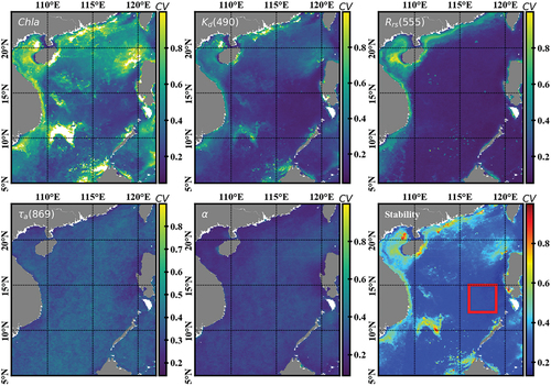
To estimate the stability of different locations and identify a wide-range target area in SCS spanning from ~5°N 105°E to ~25°N 120°E, we choose the satellite remote sensing method to evaluate temporal stability in SCS using MODIS provided atmospheric and water parameters (Zibordi and Mélin 2017). Atmospheric parameters consist of aerosol optical thickness at 869 nm (${\tau }_a\left(869\right)$) and aerosol type (α, angstrom coefficient). Water parameters consist of remote sensing reflectance at 555 nm ($R_{rs}\left(555\right)$), chlorophyll-a concentration (Chla) and diffuse attenuation coefficient at 490 nm ($K_d\left(490\right)$). $R_{rs}\left(555\right)$ is relevant to water type; Chla and $K_d\left(490\right)$ are relevant to marine bio-optical properties. We adopted the coefficient of variation (cv), which is the ratio of standard deviation (Std) to average, as the long-term stability index of each parameter. The evaluating results of all the parameters were weighted and summed to gain the combined evaluation result, and the water site was selected according to this result. The evaluating method can be represented by the following formula:

(1) $Stability=\frac{c{v}_{{\tau }_a\left(869\right)}+c{v}_{\alpha }+c{v}_{R_{rs}\left(555\right)}+c{v}_{Chla}+c{v}_{K_d\left(490\right)}}{5}$(1)

In this study, Aqua-MODIS Level-3 monthly data were downloaded from NASA’s OBPG Ocean Color website (https://oceancolor.gsfc.nasa.gov/l3/) and used for this evaluation because they are well-calibrated remote sensing data for over 20 years and can provide varied ocean color products with low uncertainties(Barnes et al. 2019; Hu, Feng, and Lee 2013).

2.2. TOA reflectance calculations

The optical signals reflected from the earth’s surface and atmosphere are received and recorded as digital numbers (DNs) by a remote sensor. If we assume that the remote sensor responds linearly to the incoming signal, the unsaturated DNs of HY-1B COCTS can be converted to TOA spectral radiance ($L_{TOA\left(i\right)}$) using calibration coefficients consisting of scaling gains and adding offsets. For a given spectrum band $i$;

(2) $L_{TOA\left(i\right)}=D{N}_{\left(i\right)}\ast a_{\left(i\right)}+b_{\left(i\right)}$(2)

where $a_{\left(i\right)}$ is the band-dependent scaling gain, and $b_{\left(i\right)}$ is the band-dependent adding offset. In-flight calibration coefficients were continuously adjusted with the radiometric responsivity degradation of the sensor. However, we used only a set of initial coefficients obtained in the first calibration activity after the launch to track responsivity degradation. In this study, the scaling, gains of eight VIS-NIR bands are 0.013,705, 0.013,545, 0.012,612,5, 0.012,55, 0.012,04, 0.010,822,5, 0.010,327,5, 0.005,897,5; all of adding offsets is zero.

The TOA radiance is then converted to TOA reflectance by:

(3) ${\rho }_{TOA\left(i\right)}=\frac{\pi L_{TOA\left(i\right)}{d}^2}{F{0}_{\left(i\right)}\ast cos{\theta }_0}$(3)

Where $d$ is the Earth-Sun distance in astronomical units, which is relevant to the date; ${\theta }_0$ is the solar zenith angle; and $F{0}_{\left(i\right)}$ is the band-dependent extra atmospheric solar irradiance (wm⁻²·sr⁻¹), which can be calculated as follows:

(4) $F{0}_{\left(i\right)}=\frac{{\int }_{{\lambda }_{i,l}}^{{\lambda }_{i,u}}F{0^{\prime }}_{\left(\lambda \right)}{\int }_{{\lambda }_{i,l}}^{{\lambda }_{i,u}}RS{R}_{\left(i,\lambda \right)}}{{\int }_{{\lambda }_{i,l}}^{{\lambda }_{i,u}}RS{R}_{\left(i,\lambda \right)}}$(4)

Where ${\lambda }_{i,l}$, ${\lambda }_{i,u}$ are the lower and upper spectral boundings of band $i$; $F{0^{\prime }}_{\left(\lambda \right)}$ is the continuous extra-atmospheric solar irradiance relevant to wavelength $\lambda$, which is a constant measured by (Thuillier et al. 2003); $RS{R}_{\left(i,\lambda \right)}$ is the continuous normalized relative spectral response function of the corresponding band $i$.

Although ${\rho }_{toa\left(i\right)}$ removes the effect of different Solar Zenith Angles (SZA), the angular effects of both the View Zenith Angle (VZA) and Relative Azimuth Angle (RAA) remain in ${\rho }_{toa\left(i\right)}$ signal. For this problem, correction based on the BRDF model is commonly used (Li et al. 2015). Unfortunately, there is also a lack of efficient BRDF-model and in-situ data on ocean targets to correct the angular effect of ${\rho }_{toa\left(i\right)}$, which varies with different angle (Ioccg 2010). For this reason, we need to rigorously select pixels of remote sensing imagery according to the limiting principle of angle that was recommended in recent research about cross-calibration of ocean color sensor that the range of SZA is ~19–50°, the range of VZA is ~25−35°, and the range of RAA is ±110–150°, which can effectively reduce the uncertainty of radiometric transform simulation and prevent sunglint contaminating (Chen et al. 2020a).

In addition, reference ${\rho }_{toa\left(i\right)}$ were generated from quasi-synchronous Terra-MODIS imageries for comparison, which has been a well-calibrated sensor and has been applied in many cross-calibration activities or accuracy evaluation of ocean color products (Butler et al. 2011; Song et al. 2019; Ye et al. 2020; Zhou et al. 2018). Note that, because of the discrepancy in $RS{R}_{\left(i,\lambda \right)}$ of various sensors, COCTS and MODIS thus may produce different ${\rho }_{toa\left(i\right)}$ results while observing same target. This effect can be reduced by using a spectral band adjustment factor (SBAF) (Chander et al. 2013), which is defined as:

$SBA{F}_{\left(i\right)}=\frac{{\int }_{{\lambda }_{i,l}}^{{\lambda }_{i,u}}RS{R^{MODIS}}_{\left(i,\lambda \right)}\ast {\rho }_{\left(\lambda \right)}/{\int }_{{\lambda }_{i,l}}^{{\lambda }_{i,u}}RS{R^{MODIS}}_{\left(i,\lambda \right)}}{{\int }_{{\lambda }_{i,l}}^{{\lambda }_{i,u}}RS{R^{COCTS}}_{\left(i,\lambda \right)}\ast {\rho }_{\left(\lambda \right)}/{\int }_{{\lambda }_{i,l}}^{{\lambda }_{i,u}}RS{R^{COCTS}}_{\left(i,\lambda \right)}}$

where ${\rho }_{\left(i,\lambda \right)}$ is the field-measured water reflectance in the open ocean and downloaded from the U.S. Geological Survey (https://crustal.usgs.gov/speclab/QueryAll07a.php).

3. Results and discussion

3.1. Stability of the selected site in SCS

A comprehensive overview of stability was provided for the site in the SCS. The stability of water and atmospheric optical properties are presented in Figure 2. Chla shows a high temporal variation in most regions. $K_d\left(490\right)$ shows consistent spatial distribution, with $CV$ values smaller than Chla. High variation appears in north and west of SCS and Luzon Strait, which receive terrestrial nutrients and upwelling (Lin et al. 2007, 2009; Pan et al. 2013; Shaw et al. 1996). The smallest $CV$ of Chla and $K_d\left(490\right)$ occurred within about 10°~ 15°N and 115°~120°E. $R_{rs}\left(555\right)$ can indicate potential changes in non-optically significant constituents in case-1 water (Zibordi and Mélin 2017). Low variation of $R_{rs}\left(555\right)$ appears in about 10° ~ 15°N and 115°~120°E, where there are no spatially consecutive or scattered high variation pixels. In the terms of atmospheric properties, the temporal variation of ${\tau }_a\left(869\right)$ and α are spatial homogeneous compared with water properties. As a result of the weighted model based on Equation (1)(1) $Stability=\frac{c{v}_{{\tau }_a\left(869\right)}+c{v}_{\alpha }+c{v}_{R_{rs}\left(555\right)}+c{v}_{Chla}+c{v}_{K_d\left(490\right)}}{5}$(1) , a sub-region in the range of 12° ~ 15°N and 116°~119°E was preliminarily selected as the stable ocean target to extract ${\rho }_{TOA\left(i\right)}$ in this study (Figure 2).

Figure 2. The CV values of surface and atmospheric optical properties and stability in the SCS. The area delineated in the red rectangular box was selected as the stable ocean target in this study.

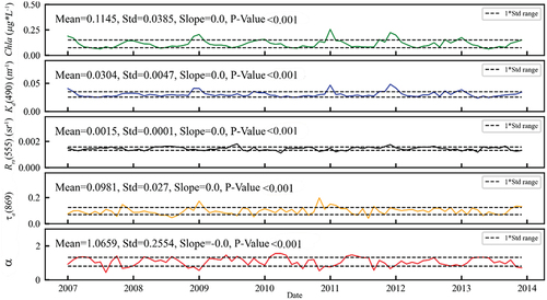
Further analysis of this subregion of 12 ~ 15°N and 116°~119°E is shown in Figure 3. The Student’s t-test was used to investigate whether the stability of the selected site was statistically significant. The null hypothesis indicates that water and atmospheric parameters change over time (slope ≠ 0, p > 0.001); otherwise, the null hypothesis is rejected, and water and atmospheric optical properties are stable. The results showed that the time-series of five parameters exhibit the slope of 0 (P-Value was close to 0), which indicates no long-term trend of growth or decline. The time-series of Chla concentration show stability with a mean of 0.11 $\mu \mathrm{g}{\mathrm{L}}^{-1}$ and Std. of 0.04 $\mu \mathrm{g}{\mathrm{L}}^{-1}$. $K_d\left(490\right)$ exhibits mean = 0.03, Std. = 0.005. $R_{rs}\left(555\right)$ time-series exhibit stability with mean = 0.0015, Std. = 0.0001. Also, ${\tau }_a\left(869\right)$ and α exhibit mean of 0.0981 and 1.06, and Std. of 0.02 and 0.25, respectively. Atmospheric properties show that this region receives a minute amount of terrestrial aerosol and is typically dominated by marine salt aerosol (Lin et al. 2007, 2009). These characteristics remain at a similar level as compared to system vicarious calibration site in the Mediterranean Sea evaluated by SeaWiFS (Sea-viewing Wide Field-of-view Sensor) level-3 data (Zibordi and Mélin 2017), which is highly consistent with MODIS (Franz et al. 2012).

Figure 3. Time-series of monthly values of water and atmospheric optical properties in the region of 12 ~ 15°N and 116°~119°E in the SCS.

3.2. Long-term trends of radiometric responsivity

The time-series of TOA reflectance ${\rho }_{toa\left(i\right)}$ over the SCS were acquired from images of COCTS between September 2007 and July 2013. The periodic oscillations were observed in these time-series for each band, as shown in Figure 4. The cycle period was approximately 1 year, which resulted from the angular effect (Li et al. 2015), and was not associated with the long-term trend of radiometric responsivity. The red fitted line for each band in Figure 4 presents the responsivity tracking result. Radiometric response degradations were observed in all bands at varying levels.

Figure 4. Time-series of TOA reflectance over SCS.

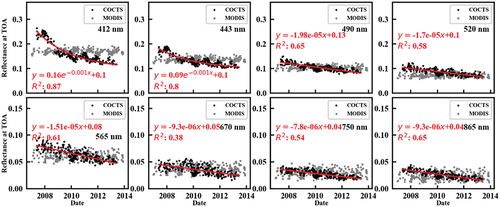
The worst degradation occurred at 412 and 443 nm bands, which temporal trend can be fitted by exponential functions. The trend lines indicated significant long-term drifts, particularly in the first 3 years of orbit. Statistics show that the annual degradation rates in these two bands were more significant than others (Figure 5). The 412 nm was the only band whose annual degradation rates reached almost 10% yr⁻¹. The 443 nm band showed second-worst degradation with 5.5% yr⁻¹. This implies the overall change during span life to be no worse than 48% and 33%, respectively. Compared with different instruments, these two bands were more stable than Fengyun-3B MERIS with an annual degradation rate of approximately 18% yr⁻¹ (Ling et al. 2013), which follows a similar optical and mechanical structure; some studies show that SeaWiFS, MODIS, MERIS exhibit higher stability, despite the potential bias due to differences in life span and evaluation methods (Chu and Wang 2020).

Figure 5. The annual mean degradation rates for each band of HY-1B COCTS.

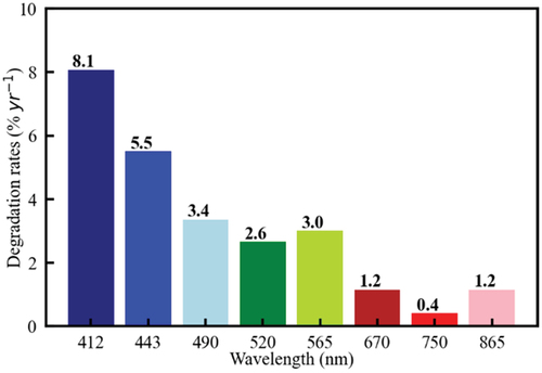
Linear regression models were used to determine the responsivity trends for other bands centered at 490, 520, 565, 670, 750, and 865 nm. Slopes of linear models indicate daily degradation ranging from −1.51×10⁻⁵ to −9.3×10⁻⁶ since the satellite launch. The responsivity degradation of these bands was weaker than 412 and 443 nm bands, and the annual degradation was 1.2%, 0.4%, and 1.2%, respectively (Figure 5).

3.3. Degradation correction of HY-1B COCTS

This section compared the spatio-temporal consistency of radiometric performance between HY-1B COCTS before/after degradation-correction and Terra MODIS. The degradation-correction coefficient was calculated following equation:

$C_{d,\lambda }=\frac{M_{0,\lambda }}{M_{d,\lambda }}$

Where $C_{d,\lambda }$ is the adjustment coefficient on a given day ($d$) and wavelength ($\lambda$). $M_{d,\lambda }$ is the degradation model (section 3.2). The radiometric magnitude of imagery was corrected by multiplying by $C_{d,\lambda }$. Note that initial calibration coefficients were inaccurate due to sensor responsivity changing in orbit, which generate TOA reflectance of HY-1B COCTS that is not significantly consistent with MODIS, especially from 412 to 565 nm (Figure 4). Rough calibration, therefore, was implemented for adjusting the initial calibration coefficients.

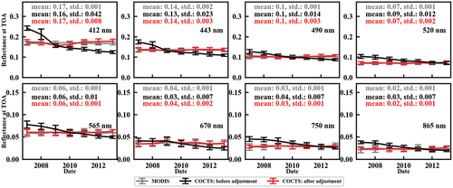
3.3.1. Temporal consistency

The temporal consistency of reflectance for TOA between HY-1B COCTS and Terra MODIS from 2007 to 2013 was further analyzed as shown in Figure 6. The improvement of the multi-sensor consistency was evident in the temporal trends. In comparison with time-series TOA reflectance before adjustment, the corrected time series have higher consistency with MODIS as their trend lines are aligned with each other. The improved variations of Std. in each year indicated trend stability of radiometric signal in a year. These improvements provide the foundation for accurate system vicarious calibration or cross-calibration. However, not all bands in their entire life achieved satisfactory accuracy. There was an apparent underestimate in 2009, and an overestimate in 2012 and 2013 at 412 nm band. Therefore, fine-tuning for a specific band in a particular period may be necessary for future research.

Figure 6. The improvement between degradation-corrected HY-1B COCTS and Terra MODIS data.

3.3.2. Spatial consistency

Cloud-free imagery of HY-1B COCTS on April 7 of 2013, at the time of worst degradation, was used to assess the radiometric performance of spatial patterns before and after degradation adjustment, and the near-simultaneous Terra MODIS imagery was used as the reference. Significant improvement for HY-1B COCTS was evident in magnitude and spatial distribution, as shown in Figure 7, especially at short-wavelength bands. The high bias of the adjusted imagery occurred in the transition zone of the “turbidity zone”, which may be caused by the degree of geometry location mismatch. Agreement between the two sensors appeared to be better in highly turbid coastal water than open mesotrophic marine, which may be caused by the lower signal-to-noise ratio of HY-1B COCTS. Note that because of the saturated signal, the spatial coverage of MODIS has been limited to turbid coastal water at 667, 748, and 865 nm bands, as shown in Figure 8. HY-1B COCTS exhibits the advantage of adequate coverage for turbid water over MODIS, which has also been pointed out in another research (He et al. 2008). To quantitatively compare the biases before and after adjustment, statistics are displayed in Table 1. Before radiometric adjustment, the means of bias at 412, 670, and 750 nm were the highest, which were 27.48%, 26%, and 26.46%, respectively. Even though the mean of bias at 865 nm band was relatively low, the standard deviation of bias exhibits the highest level, at more than 12%. A high standard deviation implies significant spatial heterogeneity, which leads to a greater difficulty of accurate radiometric calibration. The lowest means of bias were at 490 and 520 nm, with a value of 7.04% and 6.24%, respectively. Meanwhile, a similar standard deviation of bias occurred in these two bands. Overall, the mean of bias of degradation-corrected TOA reflectance was below 10% for each band, which was better than non-degradation-corrected TOA reflectance by up to almost 30%.

Figure 7. Maps of TOA reflectance on April 7 of 2013 before and after degradation adjustment of HY-1B COCTS and Terra MODIS.

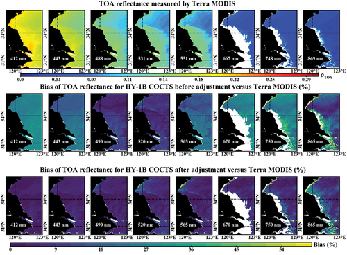
Figure 8. Maps of average bias of TOA reflectance before and after radiometric adjustment of HY-1B COCTS versus Terra MODIS.

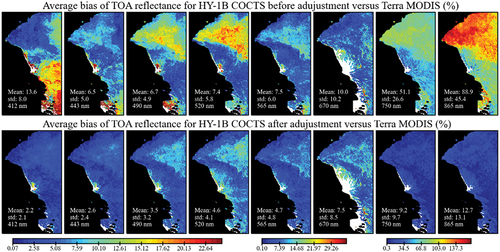
Table 1. Statistics of reflectance at TOA and bias between before and after degradation-corrected referenced Terra MODIS.

	MODIS	COCTS before adjustment			COCTS after adjustment
	${\rho }_{toa}$	${\rho }_{toa}$	Bias (%)		${\rho }_{toa}$	Bias (%)
	Mean	Mean	Mean	Std.	Mean	Mean	Std.
412 nm	0.18	0.13	27.48	2.23	0.18	2.13	1.64
443 nm	0.16	0.12	19.87	3.35	0.16	3.41	2.23
490 nm	0.12	0.11	7.04	3.86	0.12	3.31	2.76
520 nm	0.1	0.1	6.24	3.95	0.1	5.49	4.35
565 nm	0.1	0.08	17.75	4.34	0.1	3.93	4.41
670 nm	0.05	0.05	26	4.43	0.06	4.39	6.27
750 nm	0.04	0.03	26.46	7.77	0.05	6.68	14.25
865 nm	0.03	0.03	14.28	12.85	0.04	9.98	18.82

Further, we calculated the average bias of TOA reflectance of 22 cloud-free imageries between 2007 and 2013 to identify the improvement in radiometric continuity resulting from degradation correction and radiometric adjustment. As such, Figure 8 shows substantial variability in bias by data product. Specifically, ${\rho }_{toa}$ (412) and ${\rho }_{toa}$ (443) show most significant improvement with mean bias of 2.2% and 2.6%, respectively. ${\rho }_{toa}$ (750) and ${\rho }_{toa}$ (865) show most inconsistent with mean bias of 9.7% and 12.7% after radiometric adjustment, which may result in low accuracy of downstream products (remote sensing reflectance, etc.) due to their roles in atmospheric correction processing. ${\rho }_{toa}$ (490), ${\rho }_{toa}$ (520), ${\rho }_{toa}$ (565) and ${\rho }_{toa}$ (670) show moderate improvement with mean bias of 3% to 8% after radiometric adjustment. Overall, we note that general improvement in HY-1B-COCTS/Terra-MODIS continuity benefits from radiometric degradation correction and adjustment, but these changes are inconsistent for different bands and locations. Thus, accurate radiometric calibration coefficients must be acquired, which is our future work.

3.4. Degradation mechanism

The long-term response degradation rate decreases with increasing wavelength as Figure 5. Two different decay dynamics are responsible for changes in the radiometric response for each band (Eplee et al. 2012). The first decay dynamic caused a rapid degradation in response in the initial couple of years of the mission, and then the radiometric response reached a stable state. This short-term dynamic was evident in 412 and 443 nm bands. The second decay dynamic has been in effect over the entire mission, which occurs in all bands of COCTS. In terms of optical system structure, the COCTS consists of two optics instrument groups. Bands 412–565 nm were measured by a group, and their degradations were most likely caused by yellowing of the instrument optics on-orbit, which also resulted in a difference of degradation at the shorter wavelengths (bands 1–4) of SeaWiFS (Eplee et al. 2012). Bands 670–865 nm were measured by another group, and their degradation rates exhibited a similar result. Therefore, different optics instruments would cause various degradation features.

In summary, for each optics instrument group, there are two different reasons to cause degradation in the radiometric response. The first reason is the degradation of optical system degradation, consisting of lens film and photosensitive devices for each band, as the optical materials exhibit different levels of deterioration with different wavelengths. The second reason is the satellite orbit drift. Even though the solar zenith angle can be normalized in the variable of reflectance (Equation (3)(3) ${\rho }_{TOA\left(i\right)}=\frac{\pi L_{TOA\left(i\right)}{d}^2}{F{0}_{\left(i\right)}\ast cos{\theta }_0}$(3) ), the angular effect cannot be removed entirely (Kim et al. 2014; Li et al. 2015). Therefore, for the bands with a low degradation rate at the later life of the instrument when satellite orbit drifts, our research did not provide conclusive evidence that degradation was caused by optics deterioration at these bands.

4 Conclusion and future work

This paper has investigated the long-term radiometric responsivity of HY-1B COCTS visible and near-infrared bands between 2007 and 2013. A marine site was selected based on temporal stability evaluation for obtaining TOA reflectance under recommended requirements of observation geometry. Then, we used exponential or linear models to fit the degradation trend for each band. The radiometric performance exhibited continuous degradation for all bands at varying levels between 0.4% and 8.1%. The worst degradation occurred at 412 nm, with an annual average rate of 8.1%. The degradation of 443 nm reached 5.5% yr⁻¹ following 412 nm. The 490 nm, 520 nm, and 565 nm were relatively stable with a drift of 3% yr⁻¹. The red and near-infrared bands remained the most stable with the degradation of ~1% yr⁻¹. The degradation modes were used to adjust the TOA radiance for HY-1B COCTS, and then the spatial distribution of improvement was displayed in this study. The result shows that magnitude and spatial agreement between HY-1B COCTS and Terra MODIS were achieved after adjustment, which can help to improve the reliability of radiometric calibration in the lifespan of the sensor.

Note that as the previous generation ocean color satellite, HY-1B was not designed with an on-board radiometric calibration system, nor with continuous vicarious calibration based on in-situ data, which leads to the only option for evaluation of the radiometric performance of HY-1B COCTS using high-precision reference satellite sensor as Terra MODIS over a stable site. This is also common when in-situ data are unavailable for historical satellite data calibration (Pahlevan and Schott 2012; Pons et al. 2014). Terra MODIS is a well-calibrated sensor and has been widely used for cross-sensor consistency evaluation and cross-calibration. The uncertainties caused by lack of in-situ data are mainly system deviations induced by discrepancies in spectral responses and are long-term stable. Therefore, our radiometric degradation correction can be considered the relative radiometric calibration, providing a stable prior trend for low-frequency absolute calibration. In the future, the high-precise calibration method, system vicarious calibration, will be performed to meet the requirement of 0.5% spectral calibration error (Ioccg 2013), and the inherent bias in this study will be removed.

Disclosure statement

No potential conflict of interest was reported by the author(s).

Data availability statement

The HY-1B COCTS data are available on application from the National Satellite Ocean Application Service (http://www.nsoas.org.cn/). The MODIS L1B data can be obtained from the Level-1 and Atmosphere Archive and Distribution System (https://ladsweb.modaps. eosdis.nasa.gov/). The MODIS level-3 data can be obtained from Ocean Color Level 3 browser (https://oceancolor.gsfc.nasa.gov/l3/).

Correction Statement

This article has been corrected with minor changes. These changes do not impact the academic content of the article.

Additional information

Funding

This work was supported by the National Key R&D Program of China [grant numbers 2018YFB0504900 and 2018YFB0504904], the National Natural Science Foundation of China [grant numbers. 42071325 and 42176183], LIESMARS Special Research Funding, the “985 Project” of Wuhan University, and Special funds of State Key Laboratory for equipment.

Notes on contributors

Wenkai Li

Wenkai Li is currently pursuing a PhD. Degree with Wuhan University. His current research interests include the applications of remote sensing.

Guangping Xia

Guangping Xia is a postgraduate at Wuhan University. Her research interests focus on applications of remote sensing.

Qingjun Song

Qingjun Song is a researcher with the National Satellite Ocean Application Service, Ministry of Natural Resources, Beijing, China, and works on HY-1 and HY-2 series satellite instrument calibration and ocean remote sensing product validation. His research interests include remote sensing and the absolute radiometric calibration of optical instruments.

Ruqing Tong

Ruqing Tong is a postgraduate at Wuhan University. Her research interests focus on applications of remote sensing.

Liqiao Tian

Liqiao Tian is a professor at Wuhan University. His current research interest is the application of remote sensing and radiometric calibration of optical instruments.

References

- Antoine, D., P. Guevel, J.-F. Desté, G. Bécu, F. Louis, A.J. Scott, and P. Bardey. 2008. “The “BOUSSOLE” buoy—A New Transparent-to-swell Taut Mooring Dedicated to Marine Optics: Design, Tests, and Performance at Sea.” Journal of Atmospheric and Oceanic Technology 25 (6): 968–989. doi:10.1175/2007JTECHO563.1.
- Barnes, B.B., J.P. Cannizzaro, D.C. English, and C. Hu. 2019. “Validation of VIIRS and MODIS Reflectance Data in Coastal and Oceanic Waters: An Assessment of Methods.” Remote Sensing of Environment 220: 110–123. doi:10.1016/j.rse.2018.10.034.
- Butler, J.J., G. Meister, X. Xiong, B.A. Franz, and X. Gu. 2011. “Adjustments to the MODIS Terra Radiometric Calibration and Polarization Sensitivity in the 2010 Reprocessing.” Paper presented the Earth Observing Systems XVI, San Diego, CA. doi:10.1117/12.891787
- Cao, C. 2012. “Radiometric and Spectral Characterization and Comparison of the Antarctic Dome C and Sonoran Desert Sites for the Calibration and Validation of Visible and Near-infrared Radiometers.” Journal of Applied Remote Sensing 6 (1): 063541. doi:10.1117/1.Jrs.6.063541.
- Cao, C., F.J. De Luccia, X. Xiong, R. Wolfe, and F. Weng. 2014. “Early On-Orbit Performance of the Visible Infrared Imaging Radiometer Suite Onboard the Suomi National Polar-Orbiting Partnership (S-NPP) Satellite.” IEEE Transactions on Geoscience and Remote Sensing 52 (2): 1142–1156. doi:10.1109/tgrs.2013.2247768.
- Chander, G., M.O. Haque, E. Micijevic, and J.A. Barsi. 2010. “A Procedure for Radiometric Recalibration of Landsat 5 TM Reflective-Band Data.” IEEE Transactions on Geoscience and Remote Sensing 48 (1): 556–574. doi:10.1109/tgrs.2009.2026166.
- Chander, G., N. Mishra, D.L. Helder, D.B. Aaron, A. Angal, T. Choi, X. Xiong, and D.R. Doelling. 2013. “Applications of Spectral Band Adjustment Factors (SBAF) for Cross-Calibration.” IEEE Transactions on Geoscience and Remote Sensing 51 (3): 1267–1281. doi:10.1109/tgrs.2012.2228007.
- Chen, S., K. Du, Z. Lee, J. Liu, Q. Song, C. Xue, D. Wang, M. Lin, J. Tang, and C. Ma. 2020b. “Performance of COCTS in Global Ocean Color Remote Sensing.” IEEE Transactions on Geoscience and Remote Sensing 1–11. doi:10.1109/tgrs.2020.3002460.
- Chen, J., X. He, Z. Liu, N. Xu, L. Ma, Q. Xing, X. Hu, and D. Pan. 2020a. “An Approach to Cross-calibrating Multi-mission Satellite Data for the Open Ocean.” Remote Sensing of Environment 246: 111895. doi:10.1016/j.rse.2020.111895.
- Chen, S., Q. Song, C. Ma, M. Lin, J. Liu, L. Hu, S. Li, and C. Xue. 2021. “Evaluation of Regions Suitable for Vicarious Calibration of Ocean Color Satellite Sensors in the South China Sea.” Optics Express 29 (8): 11712–11727. doi:10.1364/OE.423108.
- Chu, M., and M. Wang. 2020. “The Two-Year Radiometric Evaluation of Sentinel-3A OLCI via Intersensor Comparison with SNPP VIIRS.” IEEE Transactions on Geoscience and Remote Sensing 58 (7): 4494–4500. doi:10.1109/tgrs.2019.2938974.
- Clark, D.K., M.A. Yarbrough, M. Feinholz, S. Flora, W. Broenkow, Y.S. Kim, B.C. Johnson, S.W. Brown, M. Yuen, and J.L. Mueller. 2003. “MOBY, a Radiometric Buoy for Performance Monitoring and Vicarious Calibration of Satellite Ocean Color Sensors: Measurement and Data Analysis Protocols.” Ocean Optics Protocols for Satellite Ocean Color Sensor Validation, Revision 4: 3–34.
- Eplee, R.E., G. Meister, F.S. Patt, R.A. Barnes, S.W. Bailey, B.A. Franz, and C.R. Mcclain. 2012. “On-orbit Calibration of SeaWiFS.” Applied Optics. 51 (36): 8702–8730. doi:10.1364/AO.51.008702.
- Franz, B.A., S.W. Bailey, G. Meister, and P.J. Werdell. 2012. “Quality and Consistency of the NASA Ocean Color Data Record.” Ocean Optics. doi:10.13140/2.1.2960.4169.
- Guorui, J., Z. Huijie, and L. Hao. 2014. “Uncertainty Propagation Algorithm from the Radiometric Calibration to the Restored Earth Observation Radiance.” Optics Express 22 (8): 9442–9449. doi:10.1364/OE.22.009442.
- He, X., Y. Bai, D. Pan, Q. Zhu, and F. Gong. 2008. “Primary Analysis of the Ocean Color Remote Sensing Data of the HY-1B/COCTS.” Paper presented the Remote Sensing of Inland, Coastal, and Oceanic Waters. New Caledonia. doi:10.1117/12.804839.
- He, X., Y. Bai, J. Wei, J. Ding, P. Shanmugam, D. Wang, Q. Song, and X. Huang. 2017. “Ocean Color Retrieval from MWI Onboard the Tiangong-2 Space Lab: Preliminary Results.” Optics Express 25 (20): 23955–23973. doi:10.1364/OE.25.023955.
- Helder, D.L., B. Basnet, and D.L. Morstad. 2010. “Optimized Identification of Worldwide Radiometric Pseudo-invariant Calibration Sites.” Canadian Journal of Remote Sensing 36 (5): 527–539. doi:10.5589/m10-085.
- Hu, C., L. Feng, and Z. Lee. 2013. “Uncertainties of SeaWiFS and MODIS Remote Sensing Reflectance: Implications from Clear Water Measurements.” Remote Sensing of Environment 133: 168–182. doi:10.1016/j.rse.2013.02.012.
- Hu, X., L. Wang, J. Wang, L. He, L. Chen, N. Xu, B. Tao, L. Zhang, P. Zhang, and N. Lu. 2020. “Preliminary Selection and Characterization of Pseudo-Invariant Calibration Sites in Northwest China.” Remote Sensing 12 (16): 2517. doi:10.3390/rs12162517.
- Ioccg. 2010. “Atmospheric Correction for Remotely-Sensed Ocean-Colour Products.” Reports of the International Ocean-Colour Coordinating Group (IOCCG), 78. Dartmouth, NS, Canada. doi:10.25607/OBP-101.
- Ioccg. 2013. “In-flight Calibration of Satellite Ocean-Colour Sensors.” Reports of the International Ocean Colour Coordinating Group (IOCCG), 106. Dartmouth, NS, Canada. doi:10.25607/OBP-105.
- Kim, W., T. He, D. Wang, C. Cao, and S. Liang. 2014. “Assessment of Long-Term Sensor Radiometric Degradation Using Time Series Analysis.” IEEE Transactions on Geoscience and Remote Sensing 52 (5): 2960–2976. doi:10.1109/tgrs.2013.2268161.
- Latifovic, R., J. Cihlar, and C. Jing. 2003. “A Comparison of BRDF Models for the Normalization of Satellite Optical Data to A Standard Sun-target-sensor Geometry.” IEEE Transactions on Geoscience and Remote Sensing 41 (8): 1889–1898. doi:10.1109/tgrs.2003.811557.
- Li, J., X. Chen, L. Tian, and L. Feng. 2015. “Tracking Radiometric Responsivity of Optical Sensors without On-board Calibration Systems-case of the Chinese HJ-1A/1B CCD Sensors.” Optics Express 23 (2): 1829–1847. doi:10.1364/OE.23.001829.
- Lin, I.I., J.-P. Chen, G.T.F. Wong, C.-W. Huang, and -C.-C. Lien. 2007. “Aerosol Input to the South China Sea: Results from the MODerate Resolution Imaging Spectro-radiometer, the Quick Scatterometer, and the Measurements of Pollution in the Troposphere Sensor.” Deep Sea Research Part II: Topical Studies in Oceanography 54 (14–15): 1589–1601. doi:10.1016/j.dsr2.2007.05.013.
- Lin, I.I., G.T.F. Wong, -C.-C. Lien, C.-Y. Chien, C.-W. Huang, and J.-P. Chen. 2009. “Aerosol Impact on the South China Sea Biogeochemistry: An Early Assessment from Remote Sensing.” Geophysical Research Letters 36 (17). doi:10.1029/2009gl037484.
- Ling, S., H. Xiuqing, X. Na, L. Jingjing, Z. Lijun, and R. Zhiguo. 2013. “Postlaunch Calibration of FengYun-3B MERSI Reflective Solar Bands.” IEEE Transactions on Geoscience and Remote Sensing 51 (3): 1383–1392. doi:10.1109/tgrs.2012.2217345.
- Ma, L., F. Wang, C. Wang, C. Wang, and J. Tan. 2015. “Monte Carlo Simulation of Spectral Reflectance and BRDF of the Bubble Layer in the Upper Ocean.” Optics Express 23 (19): 24274–24289. doi:10.1364/OE.23.024274.
- Men, J., J. Liu, G. Xia, T. Yue, R. Tong, L. Tian, K. Arai, and L. Wang. 2022. “Atmospheric Correction for HY-1C CZI Images Using Neural Network in Western Pacific Region.” Geo-spatial Information Science 1–13. doi:10.1080/10095020.2021.2009314.
- Pahlevan, N., and J.R. Schott. 2012. “Characterizing the Relative Calibration of Landsat-7 (ETM+) Visible Bands with Terra (MODIS) over Clear Waters: The Implications for Monitoring Water Resources.” Remote Sensing of Environment 125: 167–180. doi:10.1016/j.rse.2012.07.013.
- Pan, D., X. He, and Q. Zhu. 2004. “In-orbit Cross-calibration of HY-1A Satellite Sensor COCTS.” Chinese Science Bulletin 49 (23): 2521–2526. doi:10.1007/BF03183725.
- Pan, X., G.T.F. Wong, T.-Y. Ho, F.-K. Shiah, and H. Liu. 2013. “Remote Sensing of Picophytoplankton Distribution in the Northern South China Sea.” Remote Sensing of Environment 128: 162–175. doi:10.1016/j.rse.2012.10.014.
- Pinto, C.T., F.J. Ponzoni, R.M. Castro, L. Leigh, M. Kaewmanee, D. Aaron, and D. Helder. 2016. “Evaluation of the Uncertainty in the Spectral Band Adjustment Factor (SBAF) for Cross-calibration Using Monte Carlo Simulation.” Remote Sensing Letters 7 (9): 837–846. doi:10.1080/2150704x.2016.1190474.
- Pons, X., L. Pesquer, J. Cristóbal, and O. González-Guerrero. 2014. “Automatic and Improved Radiometric Correction of Landsat Imagery Using Reference Values from MODIS Surface Reflectance Images.” International Journal of Applied Earth Observations & Geoinformation 33 (12): 243–254. doi:10.1016/j.jag.2014.06.002.
- Ruddick, K., G. Neukermans, Q. Vanhellemont, and D. Jolivet. 2014. “Challenges and Opportunities for Geostationary Ocean Colour Remote Sensing of Regional Seas: A Review of Recent Results.” Remote Sensing of Environment 146: 63–76. doi:10.1016/j.rse.2013.07.039.
- Shaw, P.T., S.Y. Chao, K.K. Liu, S.C. Pai, and C.T. Liu. 1996. “Winter Upwelling off Luzon in the Northeastern South China Sea.” Journal of Geophysical Research Oceans 101 (C7): 16435–16448. doi:10.1029/96JC01064.
- Song, Q., S. Chen, C. Xue, M. Lin, K. Du, S. Li, C. Ma, et al. 2019. “Vicarious Calibration of COCTS-HY1C at Visible and Near-infrared Bands for Ocean Color Application.” Optics Express 27 (20): A1615–A26. doi:10.1364/OE.27.0A1615.
- Thuillier, G., M. Hersé, D. Labs, T. Foujols, W. Peetermans, D. Gillotay, P.C. Simon, and H. Mandel. 2003. “The Solar Spectral Irradiance from 200 to 2400 Nm as Measured by the SOLSPEC Spectrometer from the Atlas and Eureca Missions.” Solar Physics 214 (1): 1–22. doi:10.1023/A:1024048429145.
- Tsuchida, S., H. Yamamoto, T. Kouyama, K. Obata, F. Sakuma, T. Tachikawa, A. Kamei, et al. 2020. “Radiometric Degradation Curves for the ASTER VNIR Processing Using Vicarious and Lunar Calibrations.” Remote Sensing 12 (3): 427. doi:10.3390/rs12030427.
- Wang, D., D. Morton, J. Masek, A. Wu, J. Nagol, X. Xiong, R. Levy, E. Vermote, and R. Wolfe. 2012. “Impact of Sensor Degradation on the MODIS NDVI Time Series.” Remote Sensing of Environment 119: 55–61. doi:10.1016/j.rse.2011.12.001.
- Wu, A. 2009. “Using Dome C for Moderate Resolution Imaging Spectroradiometer Calibration Stability and Consistency.” Journal of Applied Remote Sensing 3 (1): 033520. doi:10.1117/1.3116663.
- Xiong, X., J. Sun, W. Barnes, V. Salomonson, J. Esposito, H. Erives, and B. Guenther. 2007. “Multiyear On-Orbit Calibration and Performance of Terra MODIS Reflective Solar Bands.” IEEE Transactions on Geoscience and Remote Sensing 45 (4): 879–889. doi:10.1109/tgrs.2006.890567.
- Ye, X., J. Liu, M. Lin, J. Ding, B. Zou, and Q. Song. 2020. “Global Ocean Chlorophyll-a Concentrations Derived from COCTS Onboard the HY-1C Satellite and Their Preliminary Evaluation.” IEEE Transactions on Geoscience and Remote Sensing 1–13. doi:10.1109/tgrs.2020.3036963.
- Zhi, D., W. Wei, Y. Zhang, T. Yu, Y. Pan, L. Sun, X. Li, and X. Zheng. 2019. “FengYun-3 B Satellite Medium Resolution Spectral Imager Visible On-Board Calibrator Radiometric Output Degradation Analysis.” IEEE Transactions on Geoscience and Remote Sensing 57 (6): 3240–3251. doi:10.1109/tgrs.2018.2882858.
- Zhou, Q., L. Tian, J. Li, Q. Song, and W. Li. 2018. “Radiometric Cross-Calibration of Tiangong-2 MWI Visible/NIR Channels over Aquatic Environments Using MODIS.” Remote Sensing 10 (11): 1803. doi:10.3390/rs10111803.
- Zibordi, G., and F. Mélin. 2017. “An Evaluation of Marine Regions Relevant for Ocean Color System Vicarious Calibration.” Remote Sensing of Environment 190: 122–136. doi:10.1016/j.rse.2016.11.020.
- Zibordi, G., F. Mélin, K.J. Voss, B.C. Johnson, B.A. Franz, E. Kwiatkowska, J.-P. Huot, M. Wang, and D. Antoine. 2015. “System Vicarious Calibration for Ocean Color Climate Change Applications: Requirements for in Situ Data.” Remote Sensing of Environment 159: 361–369. doi:10.1016/j.rse.2014.12.015.