Integrating geographical information systems, remote sensing, and machine learning techniques to monitor urban expansion: an application to Luanda, Angola

ABSTRACT

According to many previous studies, application of remote sensing for the complex and heterogeneous urban environments in Sub-Saharan African countries is challenging due to the spectral confusion among features caused by diversity of construction materials. Resorting to classification based on spectral indices that are expected to better highlight features of interest and to be prone to unsupervised classification, this study aims (1) to evaluate the effectiveness of index-based classification for Land Use Land Cover (LULC) using an unsupervised machine learning algorithm Product Quantized K-means (PQk-means); and (2) to monitor the urban expansion of Luanda, the capital city of Angola in a Logistic Regression Model (LRM). Comparison with state-of-the-art algorithms shows that unsupervised classification by means of spectral indices is effective for the study area and can be used for further studies. The built-up area of Luanda has increased from 94.5 km² in 2000 to 198.3 km² in 2008 and to 468.4 km² in 2018, mainly driven by the proximity to the already established residential areas and to the main roads as confirmed by the logistic regression analysis. The generated probability maps show high probability of urban growth in the areas where government had defined housing programs.

KEYWORDS:

• Land use land cover (LULC)
• spectral index
• remote sensing
• geographical information systems (GIS)
• machine learning
• PQk-means
• logistic regression

1. Introduction

Land Use Land Cover (LULC) maps are one of the bases representing the dynamic of urban environments demanding innovative concepts and techniques to obtain spatio-temporal information for urban planning (Cavur et al. 2015; Madasa, Orimoloye, and Ololade 2021; Huang et al. 2017; Orimoloye and Ololade 2020; Shao et al. 2021). LULC classification is proven to be a challenging task in remote-sensing-based urban studies due to the spectral confusion among features caused by complexity and heterogeneity of urban environments (Carranza-García, García-Gutiérrez, and Riquelme 2019; Simwanda and Murayama 2017). Very often, a single pixel of a satellite image represents multiple cover types generating confusion during classification: a mixed pixel problem that depends on the spatial resolution of the satellite image and the spatial distribution of the cover type (Choodarathnakara, Kumar, and Patil 2012). The mixed pixel problem is mainly observed in sub-Saharan African cities due to the highly complex spatial structure of the urban environment, a wide range of construction materials (Simwanda and Murayama 2017; Huang et al. 2021) along with the limited coverage of high-resolution satellite images. Although several approaches have been developed to resolve the mixed pixel in medium-resolution images, obtaining good results is still a “black box” (Trinder and Liu 2020). Most of the land-cover information extraction algorithms employ pixel-based methods, but when this approach is applied using high-resolution images, a “salt and pepper” effect is produced, contributing to a bad classification result (Huang et al. 2017). Pixel-based methods are gaining more attention for research and development with the increase of open data available on a global scale despite the emerging Very High Resolution (VHR) imagery having led to the development of object-based approaches (Lennert et al. 2019). There is no advantage using object-based classification over pixel-based classification when only medium-spatial resolution images are used (Weih and Riggan 2010; Mallinis, Plenioub, and Koutsiasb 2010; Adam, Clsapovics, and Elhaja 2016; Tassi et al. 2021). Also, the lack of spectral information necessary to discriminate spectrally similar pixels enforces the inaccuracy of the classification (Weih and Riggan 2010), which can be solved by a subpixel-based approach (MacLachlan et al. 2017). In addition, the selection of the classifier may also influence the accuracy of the classification (Cheţan, Dornik, and Urdea 2017). All the land-cover information extraction approaches mentioned above mainly resort to supervised classification. Supervised classification requires training samples and is, therefore, time-consuming, and its accuracy depends on the users’ skills. Furthermore, external factors, such as the size and quality of training samples, usually affect the performance of popular classifiers (Yang, X., and D. Shi. 2016; Huang et al. 2021). Studies in Remote Sensing (RS) often resort to band combinations that highlight features of interest (Hurd 2015). However, the land-cover information extraction from spectral indexes have also been implemented in many studies (e.g. Mwakapuja, Liwa, and Kashaigili 2013; Patel and Mukherjee 2015). Spectral indices are combinations of spectral reflectance from two or more wavelengths that indicate the relative abundance of features of interests (Harris Geospatial Solutions n.d.a). Classification based on spectral indices (Index-based classification) does not require training samples and endmembers (Li et al. 2015), reduces spectral confusion, and increases spectral contrast among different land-use classes (Xu 2007). Index-based classification also has some limitations of highlighting one specific land-cover type and confusion in discriminating some land-cover types (Li et al. 2015). To overcome this problem, Xu (2007) and Mwakapuja, Liwa, and Kashaigili (2013), by combining spectral indices, and resorting to supervised classification, extracted built-up features, vegetation, and water.

The final result of remote-sensing products can further be used to solve various problems in society. For example, from historical records of satellite images, predictive models can be generated based on change detection to understand a particular phenomenon over time, such as urban expansion and its influence in forest cover change and habitat loss. Eyoh and Nihinlola (2012), after classifying three Landsat images in Lagos, Nigeria from the years 1984, 2000, and 2005 using the K-means unsupervised algorithm, modeled, and predicted future urban expansion by employing logistic regression, considering 10 explanatory variables: distance to water, residential structures, industrial and commercial centers, major roads, railway, Lagos Island, international airport, international seaport, University of Lagos, and distance to Lagos State University. Alsharif and Pradhan (2014), by selecting distance to main active economic centers, central business district, the nearest urbanized area, educational area, roads, and to urbanized areas, easting, and northing coordinates, slope, restricted area, and population density, as possible drivers of urban sprawl, generated probability maps using data from 1984 to 2002 in the calibration phase and data from 2002 to 2010 in the validation phase resulting in an accuracy rate of 0.86. Achmad et al. (2015) predicted LULC for the year 2029 based on Banda Aceh’s (Indonesia) spatial plan regulation 2009 and 2029, by analyzing a total of seven potential driving factors.. population density, distance to central business district, green open space, historical area, river, highway, and coastal area. Traore and Watanabe (2017), integrating a Logistic Regression Model (LRM), GIS and RS, analyzed and quantified urban growth patterns and investigated its relationship with driving factors to simulate an urban growth probability map for Conakry. The results of the LRM indicated that the variables elevation and distance to major roads resulted in the best fit and the highest regression coefficients.

The synergy between GIS and RS has benefited from advances in computing, Global Positioning Systems (GPS) and Artificial Intelligence (AI) methods, particularly Machine Learning (ML), allowing massive amounts of imagery to be analyzed rapidly, outperforming more traditional tools of analysis, developed before the Big Data era (Merchant and Narumalani 2008; Vopham et al. 2018; Dangermond and Goodchild 2020) requiring higher computational costs. Cloud-based geospatial processing platforms are one of such advances that have been used for reducing computational and memory costs since the data is stored in the clouds and small portions of the data (maps, images) can be accessed upon request, manipulated on the fly resorting to built-in programming languages and ML algorithms, and the processing is done in servers owned by a big tech company or across multiple devices distributed around the world. The geospatial data-oriented cloud platform Google Earth Engine (GEE) has become the first choice for geospatial data analyses in different domains (Tamiminia et al. 2020; Yang and Huang 2021; Mao et al. 2021; Laipelt et al. 2021; Coelho et al. 2021; Junting et al. 2021) and has been used as a repository and to produce large scale LULC maps (Buchhorn et al. 2020; Karra et al. 2021; Gong et al. 2020; Midekisa et al. 2017) despite its limitations to a small number of classification and regression algorithms and inability to perform Complex machine/deep learning algorithms that need to be performed outside of its environment due to computational restrictions (Amani et al. 2020).

Remote sensing allows the collection of data from upper space and ML algorithms can help to extract knowledge from its products that can later be manipulated by overlaying with a cartographic dataset (e.g. road, river, sample points) derived from a GIS environment to produce a merged product that can be visualized for further interpretation (Merchant and Narumalani 2008; Guobin, Krakover, and Blumberg 2003; Abdollahnejad et al. 2019). ML allows systems to learn and improve automatically from experience (Awad and Khanna 2015). Experiments have shown that ML algorithms outperform parametric techniques for RS studies (with Random Forest (RF) and Support Vector Machine (SVM) achieving the best average accuracy) but, use, and implementation uncertainties limit their usage (Maxwell, Warner, and Fang 2018). In this research, to solve the mixed pixel problem, a Thematic-oriented Index Combination (TOIC) (Xu 2007; Mwakapuja, Liwa, and Kashaigili 2013) is implemented to improve the discrimination among features, which is expected to be prone to unsupervised classification. Furthermore, ML algorithms are used for: (1) classification of the satellite image using a memory and computationally efficient unsupervised classifier, Product Quantized K-means (PQk-means) (Matsui et al. 2017), to evaluate the effectiveness of index-based classification for LULC; and (2) regression (logistic regression) to monitor the urban expansion of Luanda, the capital city of Angola, for the periods of 2000–2008 and 2008–2018, having into account factors that may have driven Luanda’s urban expansion.

2. Materials and methods

2.1. Study area

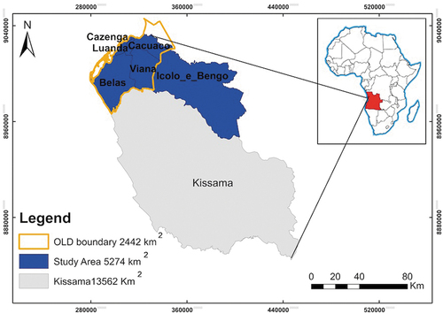
Urban growth in Luanda has increased significantly, which forced the government to expand its area in 2011 by altering the political-administrative division of Luanda and Bengo provinces (Info-Angola n.d). It is now composed of seven municipalities: Cacuaco, Belas, Cazenga, Ícolo e Bengo, Luanda, Kissama, and Viana (Figure 1). Luanda had an area of 2417 km² until 2011, increasing to 18,826 km² (GPL (Government of the Province of Luanda [Governo da Província de Luanda]) 2014), a population of 6,945,386 (INE (National Institute of Statistics [Instituto Nacional de Estatística]) 2016a), and a projected population of 7,976,907 for the year 2018 (INE (National Institute of Statistics [Instituto Nacional de Estatística]) 2016b).

Figure 1. Geographic location of the study area.

2.1.2. Urbanization in luanda

From 1948 to 1975, a series of plans failed to regulate urban expansion by the capital’s fast growth (Jenkins, Robson, and Cain 2002; Viegas 2012). After independence in 1975, the flow of rural population to the city led to a rapid expansion of informal properties. In 2002, the end of the civil war had led to an increasing search for opportunities toward improving living standards. The diagnosis of the city’s urbanization had been carried out empirically, and all proposals and interventions had been made randomly (Viegas 2012). A metropolitan plan was approved in November 2015 by the Angolan government to be developed over the next 15 years starting from 2015 (IPGUL (Luanda Urban Planning and Management Institute [Instituto de Planeamento e Gestão Urbana de Luanda]) 2015). The government intended to establish extents of 2030 (expected population 12.9 million) urban area and to impose and enforce a new urban boundary and keep sprawl in check.

2.2. Data and methods

The satellite images used in this study were obtained from different sources: NASA’s Landsat 5 Thematic Mapper (L5 TM), Landsat 7 Enhanced Thematic Mapper Plus (L7 ETM +), Landsat 8 Operational Land Imager (L8 OLI) (USGS n.d.); ESA’s Sentinel 1B (S1B) Synthetic Aperture Radar (SAR); and JAXA’s ALOS Digital Surface Model (DSM) (JAXA n.d.) (Table 1). The date of acquisition was based on availability of the satellite data that also depends on cloud coverage (trying to select images from the same month) that was also crucial for determining the period of study.

Table 1. Satellite images used in this study (L = Landsat; S = Sentinel).

Specs	L7 ETM +	L5 TM	L8 OLI	S1B	ALOS global DSM
Acq. date	2000/06/14	2008/03/24	2018/06/08	2018/06/08&13	2015/05
N^er of scenes	2	2	1	2	5
Path/Row	182/066, 067	182/066, 067	182/066		S009/E013, E014, S010/E012-E014
Acq. Orbit				Ascending
frequency				C-band 5.4 GHz
Radiometric Res.	8 bits	8 bits	16 bits	10 bits
N/bands	7	8	11	2	1
Polarization/mode				VV, VH/ IW
Data product				Level 1 GRD
Resolution	30 m rescaled to 10 m			10 m	30 m rescaled to 10 m
Source	USGS (n.d)			ESA (n.d.^b)	JAXA (n.d)

2.2.1. Preprocessing and classification

The satellite images were re-projected to the WGS84 UTM zone 33S projection system, clipped to the extent of the study area using vector data and modified according to Luanda’s new administrative division (mapcruzin n.d; Info-Angola n.d; IPGUL n.d). The Sentinel1 SAR images were radiometrically calibrated, filtered and, geometrically corrected in SNAP software using the sentinel1 toolbox. ALOS DSM (v1.1, v1.2) was used as a predictor variable for the LRM and to generate the slope raster.

The Landsat images were atmospherically corrected in QGIS 2.18. For the year 2018, Fast Line-of-sight Atmospheric Analysis of Hypercubes (FLAASH) atmospheric correction in ENVI software resulted in a better performance of the classifier (see the comparison in supplementary material). BQA bands from the three Landsat data were used to remove clouds from the scenes masking out values higher than 672 for Landsat 5 and 7 and 2720 for Landsat 8 according to convenience, since getting rid of clouds is paramount for the proposed classification approach.

2.2.2. Calculation of spectral indexes from Landsat 8 data

Five spectral indexes, Normalized Difference Built-up Index (NDBI), Moisture Enhancement Index (MEI) (Liau 2016), Vegetation Index considering Green and Shortwave Infrared (VIGS) (Hede et al. 2015), Dry Built-up index (DBI) (Rasul et al. 2018) and an empirical built-up index QzCal were calculated and used as input for the unsupervised classification. Additionally, SAR data (VV and VH polarized bands) were added to improve the classification.

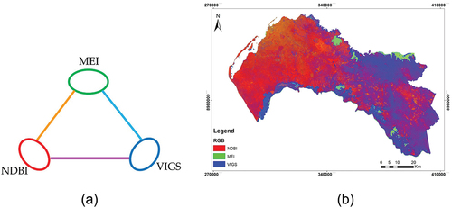
For the 2018 image, the main initial idea was to select a built-up/bareland index, a water index, and a vegetation index, to discriminate the four LULC classes, having preference to spectral indexes that outperform conventional spectral indexes: NDBI; MEI instead of Normalized Difference Water Index (NDWI [Gao 1996]); and VIGS instead of Normalized Difference Vegetation Index (NDVI) or Soil Adjusted Vegetation Index (SAVI [Huete 1988]) (Figure 2(a,b)).

Figure 2. (a) Spectral index combination. (b) Composite image of NDBI, MEI, and VIGS.

NDBI (Equation (1)(1) $NDBI=\frac{SWIR-NIR}{SWIR+NIR}$(1) ) enhances built-up/Bareground by applying the difference between Short-Wave Infrared (SWIR) and Near-Infrared (NIR).

(1) $NDBI=\frac{SWIR-NIR}{SWIR+NIR}$(1)

MEI combines three spectral indexes to handle their weak differences (Equation (2)(2) $MEI=\frac{Green-NIR}{Green+NIR}+\frac{Green-SWIR1}{Green+SWIR1}+3\times \frac{Band1-Green}{Band1+Green}$(2) ). The first two indexes, NDWI (McFeeters 1996) and Modified Normalized Difference Water Index (Xu 2007, 2008), enhance the water category by eliminating vegetation objects (higher reflectance in NIR and SWIR1 bands (Landsat 8) compared to the Green band while water reflects few differences). The third index eliminates urban/bareground reflectance by applying the difference between band 1 of Landsat 8 (coastal aerosol) and the green band (higher reflectance in the green band compared to the coastal aerosol band) while water reflects few differences.

(2) $MEI=\frac{Green-NIR}{Green+NIR}+\frac{Green-SWIR1}{Green+SWIR1}+3\times \frac{Band1-Green}{Band1+Green}$(2)

Atmospheric and ground-surface conditions, such as clouds and soils, often distort NDVI accuracy in detecting vegetation (Shishir and Tsuyuzaki 2018). SAVI is more sensitive than NDVI in detecting vegetation in the low-plant covered areas as low as 15%, while the NDVI can only work effectively in the area with plant cover above 30% (Xu 2008). Given NDVI and SAVI’s limitations, VIGS, developed to discriminate unhealthy from healthy vegetation stressed by heavy metals in an area covered by thick vegetation, was chosen. VIGS combines 1) two spectral indexes, Green-Red and NDVI, to discriminate vegetation from other backgrounds; and 2) one spectral index NDWI (Gao 1996) to discriminate water from other backgrounds (Equation (3)(3) $VIGS=\frac{Green-Red}{Green+Red}+0.5\times \frac{NIR-Red}{NIR+Red}+1.5\times \frac{NIR-SWIR1}{NIR+SWIR1}+1.5\times \frac{NIR-SWIR2}{NIR+SWIR2}$(3) ). Since SWIR reflectance is sensitive to leaf water content (Hede et al. 2015), following the same idea as MEI, there is a hypothesis that VIGS in an area with non-thick vegetation may enhance vegetation and water categories (higher values) while eliminating urban/bareground (lower values).

(3) $VIGS=\frac{Green-Red}{Green+Red}+0.5\times \frac{NIR-Red}{NIR+Red}+1.5\times \frac{NIR-SWIR1}{NIR+SWIR1}+1.5\times \frac{NIR-SWIR2}{NIR+SWIR2}$(3)

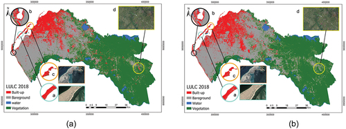
An experimental unsupervised classification for the band combination NDBI, MEI, VIGS is illustrated in Figure 3(a). The classified map still had some misclassification when discriminating bareground from built-up areas (Figure 3(a) in Figure 3). A fieldwork in Luanda aimed to visit the misclassified points (Figure 3(b,d) in Figure 3(a)) to understand the diversity of the surrounding features and how they respond to spectral indexes.

Figure 3. LULC map 2018 from PQk-means algorithm. (a) using the spectral indexes NDBI, MEI, VIGS. (b) using the spectral indexes NDBI, MEI, VIGS, DBI, and QzCal. In (a, b) sub-figures a and c show the Sand beach misclassified as built-up, b shows the saline area misclassified as built-up, d shows the built-up misclassification in agriculture field. d in Figure (b) shows improved result.

Trying to discriminate sand beach from built-up, which has been misclassified in the first experimental classification, an empirical spectral index was calculated: Quartz and Calcite are principal constituents of beaches in tropical and sub-tropical seas (Vincent 1997, 14). The spectral reflectance for Quartz and Calcite in TIR (range 10.6–11.19 µm wavelength for Landsat 8 TIR1 band) is higher compared to their spectral reflectance in SWIR (both, 2.1 µm wavelength, which is within the Landsat 8 SWIR2 band range). Based on this assumption, the normal difference between Landsat 8 TIR1 and SWIR2 bands, here referred to as QzCal spectral index (eEquation (4)), was calculated to discriminate sand beach from other backgrounds. An additional spectral index, dry built-up index (DBI) (Equation (5)(5) $DBI=\left(Blue-\frac{TIR1}{Blue}+TIR1\right)-NDVI$(5) ) (Rasul et al. 2018) was calculated which together with QzCal, improved the classification result (Figure 3(d)) but built-up class was still misclassified (figures (a-c) in Figure 3(b)).

(4) $QzCal=\frac{TIR-SWIR2}{TIR+SWIR2}$(4)

(5) $DBI=\left(Blue-\frac{TIR1}{Blue}+TIR1\right)-NDVI$(5)

Since the result was still not satisfactory, 10 m resolution Sentinel-1 C-Bands (VV+VH) were added to improve the classification (Corbane et al. 2008; Abdikan et al. 2016; Sinha, Santra, and Mitra 2018). The reason is to take advantage of the double-bounce effect on built-up features from SAR data (Tavares et al. 2019). The final selection of spectral indexes was based on their performance regarding the diversity of spectral reflectance in the study area: NDBI, MEI, VIGS, DBI, QzCal, and two sentinel SAR bands resulting in 7 input data.

2.2.3. Classification algorithm

For the Landsat 8 OLI image, which provides unique specifications, such as radiometric resolution of 16 bits, and the aerosol band that is important for the calculation of one of the spectral indexes, a memory and computationally efficient unsupervised classifier, i.e. PQk-means was chosen. PQk-means first compresses input vectors into memory-efficient short codes by product quantization and then clusters the resultant product-quantized (Pq) codes in the compressed domain (Matsui et al. 2017). As with K-means (Harris Geospatial Solutions n.d.b), PQk-means finds the nearest center from each code and updates each center using a proposed sparse voting scheme (Matsui et al. 2017). The optimization process consisted of keeping the same dimension of the input because the dimension represents an odd number (seven input bands) (num_subdim = 7); setting the Pq-code to eight bits (Ks = 256); quantizing the original dataset (7 × 52,535,364-pixel) to only 5,000,000-pixel; and finally setting the number of classes to eight, a higher number than the expected number of classes desired for the classification, that were in a later stage merged into four classes.

The resulting PQk-means LULC map was compared with classified maps from state-of-the-art unsupervised K-means classifier available in python scikit-learn library, and supervised SVM classifier in ArcGIS Pro. The comparison with the supervised approach SVM was performed using the band combination NIR, SWIR, and red. For previous Landsat mission data (Landsat 7 for the year 2000 and Landsat 5 for the year 2008), which lack some important specifications mentioned earlier, supervised Maximum Likelihood Classification (MLC) and SVM respectively, were performed in ArcGIS Pro, also using the band combination NIR, SWIR, and red. The choice of the classifier for each case was based on performance when compared to other classification techniques (Huang et al. 2018).

2.2.4. Accuracy assessment

The accuracy assessment was conducted in QGIS using the Accuracy Assessment of Thematic Maps (AcATaMa) plugin (Corredor 2018). Despite being easy to use, the AcATama plugin does not provide the K coefficient, which is an important parameter to test interrater reliability (McHugh 2012). For this reason, the confusion matrix tool in ArcGIS Pro was used to determine the K coefficient. In total, 160 stratified random points (40 per class) were generated for the 2000 and 2008 classified images (Corredor 2018; Olofsson et al. 2013). For the 2018 image, 480 stratified random points (120 per class) were generated. To the random points generated, ground truth labels were assigned through visual interpretation having assistance from TOIC (NDBI, MEI, and VIGS), true-color composite (red, green, and blue) and false-color composite (NIR, SWIR, and red) of the same Landsat image used for classification each year (see supplementary material Figures 16).

2.2.5. Predictive model (logistic regression)

Different urban growth models consider different indicators to predict urban growth phenomena (Musa, Hashim, and Reba 2016). No single model appears to perform consistently well when applied to different geographical locations (Xie et al. 2005). Logistic regression empirically uses statistical techniques to model the relationship between LULC changes and drivers based on historical data (Atak et al. 2014). The $logit\left(Y\right)$ function (Equation (6)(6) $logit\left(Y\right)={\beta }_0+{\sum }_{i=1}^n\beta x_i$(6) ), a linear combination function of the explanatory variables was, used to carry out the logistic regression model (Li 2017).

(6) $logit\left(Y\right)={\beta }_0+{\sum }_{i=1}^n\beta x_i$(6)

where x_i is the explanatory variable, β_i is the regression coefficient to be estimated, and β₀ is the intercept.

2.2.5.1. Dependent variable

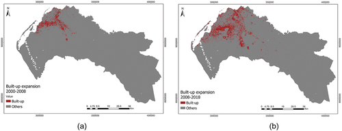
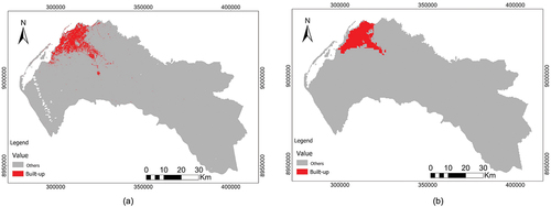
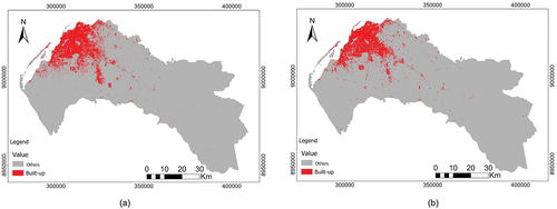
The LULC classified maps of 2000, 2008, and 2018 were used to generate the dependent variables for the models. A binary map representing the change in built-up during the period 2000–2008 was used as input for the first model (Figure 4(a)). The same procedure was used for the model corresponding to the period 2008–2018 (Figure 4(b)).

Figure 4. (a) Binary map representing expansion from 2000 to 2008. (b) Binary map representing expansion from 2008 to 2018.

2.2.5.2. Independent variables

There is no rule or known global formula for selecting land-use drivers (Eyoh and Nihinlola 2012; Akinwande, Dikko, and Samson 2015). Predictors were selected a priori based on previous studies in African cities (Eyoh and Nihinlola 2012; Traore and Watanabe 2017), the current knowledge of the urbanization processes in the study area, as well as the results from hypothesized driving forces of urban growth (Atak et al. 2014).

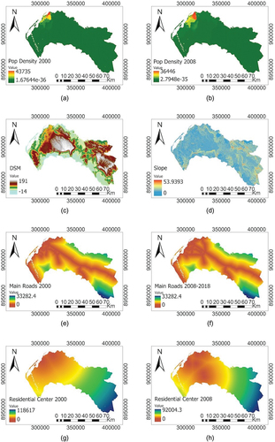
Seven initial drivers were chosen: (1) population density (Forum-angonet n.d; INE (National Institute of Statistics [Instituto Nacional de Estatística]) 2016a; INE (National Institute of Statistics [Instituto Nacional de Estatística]) 2016b), (2) elevation (JAXA n.d.), (3) Slope, distance to (4) the main roads (mapcruzin n.d.), (5) residential areas, (6) industrial areas, and (7) primary centers (IPGUL (Luanda Urban Planning and Management Institute [Instituto de Planeamento e Gestão Urbana de Luanda]) 2015) (see supplementary material Figure S5.2), but only the first five were selected to generate the models (Figure 5).

Figure 5. Independent variables: (a) Population density (2000). (b) Population density (2008). (c) Digital Surface Model. (d) Slope. (e) Distance to main roads (2000). (f) Distance to main roads (2008–2018). (g) Distance to residential center (2000). (h) Distance toresidential center (2008).

2.2.5.3. Multicollinearity

Before any regression analysis, multicollinearity should be checked. Eliminating a variable involved in collinearity runs the risk of omitted variable bias (Lesschen, Verburg, and Staal 2005). Variance inflation factor (VIF) (Equation (7)(7) $VIF=\frac{1}{1-R^2}$(7) ) is the most widely used diagnostic for multicollinearity that may be calculated for each predictor by doing a linear regression of that predictor on all the other predictors and obtaining the R² from the regression (Allison 2012). VIF determines how much the variance of an estimated regression coefficient increases when predictors are correlated (Akinwande, Dikko, and Samson 2015). A Pearson correlation analysis among predictor variables was conducted prior to the logistic regression modeling, followed by VIF analysis (Tavares 2017).

(7) $VIF=\frac{1}{1-R^2}$(7)

2.2.5.4 Model evaluation

The coefficient of determination R² is used as a standard to measure the overall strength of a linear regression model, with zero indicating a model with no predictive value and one indicating a perfect fit (Hu, Palta, and Shao 2006). Several goodness-of-fit indexes, also known as “pseudo-R²” analogs of R² as used in Ordinary Least-Squares (OLS) regression, exist to assess the predictive capacity of the logistic regression model. One such index, McFadden pseudo-R² (Equation (8)(8) $R_{MF}^2=1-\frac{LL\left(Full\right)}{LL\left(Null\right)}$(8) ), is perhaps the most popular pseudo-R² index (Smith and McKenna 2013; Williams 2015).

(8) $R_{MF}^2=1-\frac{LL\left(Full\right)}{LL\left(Null\right)}$(8)

where LL(Full) is the full-model log-likelihood, and LL(Null) is the intercept-only log-likelihood. For two models performed on the same data, the greater the likelihood, the higher McFadden’s pseudo-R² (UCLA 2011).

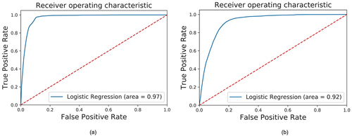
Another index, Receiving Operating Characteristic (ROC), represented by the area under the curve (AUC), measures the relationship between expected and real changes (Alsharif and Pradhan 2014). ROC graphically represents “true positive” and “false positive” classification rates as a function of different classification cutoff values for the predicted probabilities resulting from the logistic regression (Smith and McKenna 2013).

3. Results and discussion

3.1. Unsupervised classification

A major challenge in unsupervised learning is evaluating if the algorithm learned something useful, and often, the only way to evaluate its result is to inspect it manually (Muller and Guido 2017). A comparison of the PQk-means classified map with maps from state-of-the-art classification techniques, K-means and SVM (see also RF and MLC in supplementary material Figure 7.2(a, b)) was made by performing accuracy assessment using the same ground truth. For the 2018 images, 93% and 95% of overall accuracy were achieved corresponding to PQk-means and K-means unsupervised algorithms, respectively, and from the supervised classification, 89%, 87%, and 78% of overall accuracy were achieved using SVM, RF, and MLC algorithms, respectively (Figures 6(a,b), 7 and Figure S7.2 in supplementary material; Table 2 and Table S2.2 in supplementary material).

Figure 6. LULC map 2018 using the spectral indexes NDBI, MEI, VIGS, DBI, QzCal, and two SAR polarized bands. (a) PQk-means classification. (b) K-means classification. In Figure (a) and, (b), sub-figure a shows the improved classification of built-up area; b shows the improved classification in saline area; c shows the improved classification of built-up in sand beach area; d shows the reduced overestimation of built-up in a rough surface area.

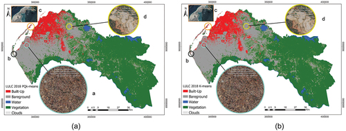
Figure 7. LULC map 2018 from SVM algorithm using the Landsat 8 band combination NIR, SWIR1, red (564). (a) underestimated built-up area (b) saline area classified as built-up, (c) improved classification of built-up in a sand beach area, (d) overestimation of built-up in a rough surface area.

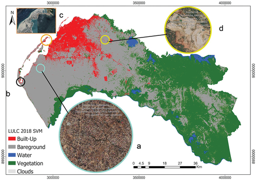
Table 2. Accuracy assessment and quantification of LULC 2000, 2008, 2018 (PQk-means), 2018 (K-means) and 2018 (SVM).

Class	User accuracy	Area(km^2)	Percentage (%)
Built-up	0.77–0.70-0.97–0.97–0.96	94.53–198.29-468.37–489.88-441.86	1.80–3.77-8.91–9.32-8.38
Bareground	0.97–0.97-0.95–0.93–0.71	2412.20–1806.52-1682.94–1886.03-2467.11	45.97–34.43-32.03–35.90-47.12
Water	1.00–1.00–1.00–1.0–1.0	148.90–144.90-131.51–130.76-126.29	2.83–2.76-2.50–2.48-2.39
Vegetation	0.67–0.92-0.85–0.92-0.97	2591.39–3097.31-2970.70–2746.84-2218.25	49.38–59.03-56.54–52.28-42.09
Total		5247–5247-5253-5253-5253
O.Accuracy:	0.82–0.93–0.93-0.95-0.89
Kappa	0.76–0.91–0.91–0.94–0.85

The K-means algorithm was also used to validate the PQk-means computational efficiency, although PQk-means memory efficiency from this comparison could not be proved: While K-means took more than half a day to classify a large scale 7 × 52,535,364-pixel image, PQk-means only took approximately 16 minutes running on a machine with Intel Core i5 of 3.3 GHz and 8 GB memory.

Below, the spectral profiles of the four classes, are represented in parallel coordinates for the bands, NIR, SWIR, red, green (Figure 8(a)), and the spectral indexes used in unsupervised classification (Figure 8(b)).

Figure 8. (a) Spectral profile Landsat 8 Bands 6, 5, 4, 3. (b) Spectral profile for the five spectral indexes and 2 SAR polarized bands.

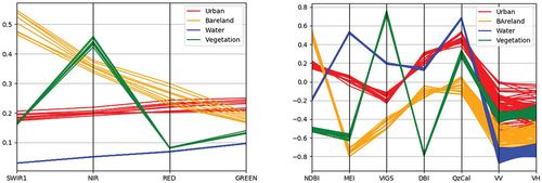
While the first spectral profile only shows the discrimination in four bands, the second one shows a more diverse feature discrimination. It can easily be seen how well the separability was in both spectral profiles. Although the second one still has some confusion in the SAR polarized bands, it allows us to see the unseen in seven dimensions. For the built-up class, false alarms on SAR image correspond to areas where backscattering greatly varies, like fields with rough bare soils (sub-figure (d) in Figures 6(a,b) and 7) or with high soil moisture content. The build-up underestimation in the classified maps is essentially related to the presence of some low-density urban areas (sub-figure (a) in Figures 6(a) and 7) that do not face the radar beam and accordingly have a low return signal (Corbane et al. 2008). A higher underestimation of the built-up class can be observed on the SVM map in which only optical data were used (sub-figure (a) in Figure 7).

It is common that after improvement methods, built-up areas still get confused with everything since urban is extremely heterogeneous spectrally (NASA (National Aeronautics and Space Administration) 2017). The goal of this study was not necessarily to outperform conventional classification techniques. Instead, the interest was to find a solution for the spectral confusion of built-up areas in the Sub-Saharan African countries and find an alternative for the time-consuming supervised classification.

3.2. Supervised classification

Figure 9(a and b) represent the results from the supervised classification whose accuracy assessment resulted in 82% and 93% for the images corresponding to the years 2000 and 2008, respectively (Tables 2 and 3). Let’s clarify that the bareground here referred does not correspond to pixels representing exclusively bareground. With 30 m resolution satellite images, individual pixels covering suburban area will represent a mixture of buildings, vegetation, and bareground (Smith and Hoffmann 2000), and the similarity of the spectral reflectance of soil and non-photosynthetic vegetation in the Visible-NIR (VNIR) spectral region may underestimate regional scale total vegetation cover (Gill and Phinn 2008). Bareground pixels may contain vegetation but were assigned to the class label with the maximum proportion of the pixel (Chen et al. 2018). The discrimination of bareground and vegetation is probably the drawback of the index-based unsupervised classification, which is not a big problem for proceeding to the second objective of this study focused on built-up class.

Figure 9. (a) LULC map 2000 from MLC. (b) LULC map 2008 from SVM.

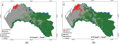
Table 3. Correlation of the predictor variables for model 1 (2000–2008) after removing predictors with high VIF. Road for the year 2000 (Rd_2000). Residential area for the year 2000 (Rsd_2000), DSM, Slope and Population Density for the year 2000 (PD_2000).

	Rd_2000	Rsd_2000	DSM	Slope	PD_2008	VIF
Rd_2000	1.00	0.50	–0.30	0.06	–0.18	1.50
Rsd_2008	0.50	1.00	–0.01	0.18	–0.25	1.40
DSM	–0.30	–0.01	1.00	0.03	–0.04	1.00
Slope	0.06	0.18	0.03	1.00	–0.04	1.00
PD_2008	–0.18	–0.25	–0.04	–0.04	1.00	1.10

3.3. Built-up area estimation

After classification and assessment of accuracy, the different LULC classes were quantified (Table 2; Figure 10(a and b)). It is important to clarify that the total study area from the different classification results slightly differs because of removed clouds’ pixels. Apart from the overall accuracy, the user’s accuracy should be paid attention to understand which classes resulted in fewer false alarms (Cao et al. 2018). The user accuracy of the built-up class for 2018 is high and slightly differs among the three classification approaches: 97% for PQk-means and K-means and 96% for SVM (Table 2).

Figure 10. (a) Built-up expansion from 2000 to 2018. (b) LULC change quantification.

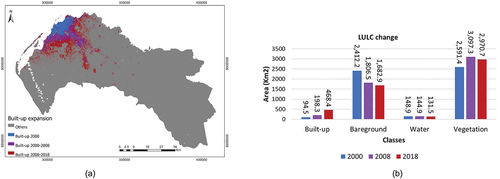
The estimated built-up area for the year 2000 is around 94 km², while the Atlas of Urban Expansion (AUE) of Angel et al. (2016) estimated the built-up area to be 171.75 km² in 2000. The AUE differentiates the built-up pixels classified in the Landsat imagery into three types: (1) urban, when the majority of built-up pixels (50% or more) are within the Walking Distance Circle (WDC), defined as a circle with area 1 km² and radius 584 m; (2) suburban, (25–50% of built-up pixels in their WDC); and (3) rural (less than 25% of build-up pixels in their WDC). The threshold for this three-fold division is somewhat arbitrary, that might be the reason for such a significant difference between the classified map for the year 2000, and the AUE built-up estimation since the share of a class in each pixel within the WDC is not taken into account in this study.

For the year 2008, the estimated built-up area is around 197 km² (Figure 11(a)) while the map based on Envisat MERIS fine resolution 300 m image of 2009 (Figure 11(b)), (Arino et al. 2012) estimates 207 km² (check geodatabase Globcover dataset in supplementary material).

Figure 11. (a) Built-up map 2008, (b) Built-up map 2009 based on Envisat Meris (Arino et al. 2012).

For 2018, the estimated built-up area is 468 km² (Figure 12(a)) that is comparable with the 407 km² of the 2015/2016 built-up area estimated by ESA (2017) on its high-resolution prototype map of Africa (Figure 12(b)).

Figure 12. (a) Built-up map 2018 from PQk-means classification, (b) Built-up map 2015/2016 from high-resolution prototype map of Africa (ESA 2017).

3.4. Logistic regression

The results of the Pearson correlation analysis for the models corresponding to the periods 2000–2008 (model 1) and 2008–2018 (model 2) show a very high correlation among the variables of distance to residential areas, to industrial areas, and to the primary center (supplementary material Tables 3.2 and 4.2). After checking for multicollinearity, some researchers consider 2.5 as a threshold for VIF (Allison 2012), and others only include values close to 5.0 if the variable in case is a suppressor variable, i.e. a variable that is not correlated with the dependent variable but is significantly correlated with other independent variables improving the overall predictive power (Akinwande, Dikko, and Samson 2015). In this study, no suppressor variable was found (see supplementary material Tables 3.2 and 4.2), and satisfactory result was achieved after removing two of the three variables with high correlation (distance to primary center first and distance to industrial areas) (Tables 3 and 4).

Both models with pseudo R² equal to 0.476 (Model 1) and 0.36 (Model 2) show a very good fit (Tables 5–6): Pseudo-R² values between 0.2 and 0.4 represent a very good fit of the model (Lee 2013).

Table 4. Correlation of the predictor variables for model 2 (2008–2018) after removing predictors with high VIF. Road for the years 2008 and 2018 (Rd_2008_2018), Residential area for the year 2008 (Rsd_2008), DSM, Slope and Population Density for the year 2008 (PD_2008).

	Rd_2008_2018	Rsd_2008	DSM	Slope	PD_2008	VIF
Rd_2008_2018	1.00	0.53	–0.31	0.06	–0.23	1.60
Rsd_2008	0.53	1.00	–0.01	0.19	–0.30	1.60
DSM	–0.31	–0.01	1.00	0.03	–0.03	1.20
Slope	0.06	0.19	0.03	1.00	–0.06	1.00
PD_2008	–0.23	–0.30	–0.03	–0.06	1.00	1.10

Table 5. Logistic regression results for model 1 (2000–2008). Const – intercept in the logit function, Coef – coeficient of the intercept (in the case of the first value) and the predictor variables, Std.Err – standard error, P>|s| – p value associated with z-score z, [025 0.975] – confidence interval; Road for the year 2000 (Rd_2000), Residencial area for the year 2000 (Rsd_2000), DSM, Slope and Population Density for the year 2000 (PD_2000).

	Coef.	Std.Err	z	P>|z|	[0.025	0.975]
Const	−2.11	0.02	−100.54	0.0000	−2.15	−2.07
Rd_2000	−16.77	0.09	−170.66	0.0000	−16.96	−16.58
Rsd_2000	−28.13	0.11	−244.64	0.0000	−28.35	−27.90
DSM	7.13	0.05	146.89	0.0000	7.03	7.22
Slope	−2.99	0.10	−28.21	0.0000	−3.20	−2.79
PD_2000	−1.69	0.02	−85.68	0.0000	−1.73	−1.65

The AUC shows a very high power for distinguishing the two classes (built-up and non-built-up) in model 1 (97%), while in model 2 it shows a moderate discriminatory power (92%) (Figure 13(a and b)). In general, ROC curves with an AUC ≤ 75% are not clinically useful, and an AUC between 75% and 97% has moderate discriminatory power, while a ROC curve with an AUC of 97% has a very high clinical value (Fan, Upadhye, and Worster 2006).

Figure 13. (a) ROC curve of Model 1, (b) ROC curve of Model 2.

All the P-values lower than 0.05 and its associated z values greater than 1.96 for positive z and less than −1.96 for negative z, show the importance of the predictor variables used in the two models in explaining urban expansion (Tables 5 and 6), which means that the null hypothesis was not satisfied for any predictor variable, allowing us to infer that urban expansion in Luanda is mainly driven by the proximity to (1) already established residential areas and (2) to the main roads that are confirmed by their higher coefficients in both models (negative relationship with distance to main roads and to residential areas).

Table 6. Logistic regression results for model 2 (2008–2018). Const – intercept in the logit function, Coef – coefficient of the intercept (in the case of the first value) and the predictor variables, Std.Err – standard error, P>|s| – p value associated with z-score z, [025 0.975] – confidence interval; Road for the years 2008 and 2018 (Rd_2008_2018), Residential area for the year 2008 (Rsd_2008), DSM, Slope and Population Density for the year 2008 (PD_2008).

	Coef.	Std.Err	z	P>|z|	[0.025	0.975]
Const	1.09	0.01	103.40	0.0000	1.07	1.12
Rd_2008	–9.81	0.04	–260.87	0.0000	–9.88	–9.73
Rsd_2008	–12.39	0.03	–359.58	0.0000	–12.46	–12.32
DSM	–1.57	0.01	–101.44	0.0000	–1.56	–1.54
Slope	0.69	0.05	13.93	0.0000	0.59	0.79
PD_2008	–1.48	0.01	–105.96	0.0000	–1.50	–1.45

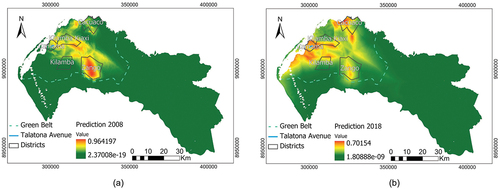
From the probability maps, especially the one corresponding to 2018, areas with a higher probability of urban growth can be observed in places where the government had defined housing programs: Talatona in Camama district, Kilamba Kiaxi, Zango, Cacuaco (GPL (Government of the Province of Luanda [Governo da Província de Luanda]) 2014; IPGUL (Luanda Urban Planning and Management Institute [Instituto de Planeamento e Gestão Urbana de Luanda]) 2015) and Kilamba (Figure 14(a and b)).

Figure 14. (a) Probability map 2008 from model 1. (b) Probability map 2018 from model 2.

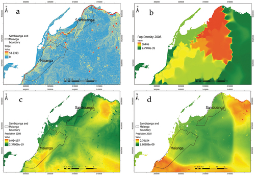
The variable elevation changes from a positive and high influence on urban expansion to a negative and low influence, while the variable slope changes from a negative and low influence to a positive and still low influence during the period 2000–2018 (Tables 5 and 6). This trend might be because during the period 2000–2008 with a small urban area concentrated near the shore (west), where the elevation is low, people were more likely to build far from these areas, avoiding areas with high densities of people and areas at risk most affected by slope such as Sambizanga and Maianga from the old administrative division of Luanda (Mendelsohn, Mendelsohn, and Nakanyete 2010) (Figures 14(a) and 15(a–d), having preference for already built residential areas near the main roads for easy access to services. During the period 2008–2018, with the urban growth, inhabitants were forced to shape their priorities within the metropolitan area, having chosen to fill low elevation and high-risk areas (higher slope) rather than already built and populated (negative relationship) areas and near the main roads (Figures 14(b), 15(a, b and d)).

Figure 15. (a) The slope in the areas of Maianga and Sambizanga. (b) detail of the corresponding probability map for the year 2008. (c) detail of population density for the year 2008. (d) detail of population density for the year 2018.

For the future metropolitan plan, the proposed transport network was designated as development corridors reserved for new dense and high-quality development (Mobility in chain 2015) and is expected to become the main driver of the urban development since we have confirmed with our results that government-imposed rules have determined the way the built-up stain looks like today. The result of this study will be beneficial for environmentalists and urban planners, to understand and monitor the urban dynamic since the methods can easily be reproduced with new input data, and to inspire researchers toward machine learning application to GIS/RS.

3.5. Limitations of the study

Data availability has limited the methodology of this study to be implemented with previous satellite data, for example, the usage of SAR data for the years 2000 and 2008. There are commercial SAR data providers, but relying on commercial datasets can consume monetary resources, since it does not guarantee that the data will certainly be useful.

Future built-up area expansion could not be predicted from the logistic regression because it is believed that future prediction may lead to errors. This is because urban expansion drivers constantly change their predictive power, and some drivers can be removed, or new drivers be introduced over time. An approach that considers previous models, i.e. sequence models such as Recurrent Neural Network (RNN), could be a better approach for future prediction.

4. Conclusions

The results of this study show that unsupervised classification utilizing spectral indexes can effectively classify LULC if appropriate spectral indices and classifiers are chosen for a specific area. For unsupervised LULC classification, the K-means algorithm is preferred. However, considering a large number of inputs (spectral indexes), PQk-means, that to the best of found knowledge, was implemented for the first time in RS studies, is an alternative selection because it is memory and computationally more efficient, and gives good accuracy similar to K-means.

The built-up area of Luanda during the period 2000–2018 was mainly driven by the proximity to the already established residential areas and to the main roads, with other drivers playing an important role in urban expansion when changing from a positive to negative influence or vice-versa, as a consequence of newly dense built-up areas and rules imposed by the government. In future research, it would be interesting to see the predictive performance of the emerging deep learning algorithms such as Long Short Term Memory (LSTM) using the same approach of this study.

Acknowledgments

We gratefully acknowledge Professor Takayuki Shiraiwa from the Institute of Low Temperature Science, Hokkaido University, for his precious inputs in the design of the research; Professor Katsuaki Koike from the Department of Urban Management, Graduate School of Engineering, Kyoto University, for a great discussion on spectral indices; Koki Kasai, a former Ph.D. student from the Graduate School of Information Science and Technology, Hokkaido University, for the tips and suggestions on which Python libraries to use to handle satellite images, which is simple but was crucial for this research; and the anonymous reviewers whose suggestions contributed for the improvement of this manuscript.

Data availability statement

The data that support the findings of this study are available in Mendeley data repository at http://dx.doi.org/10.17632/hkfxnm2xpk.1, under a Creative Commons Attribution 4.0 International license and the codes at https://github.com/arngolo/Integrating-GIS-RemoteSensing-ML-for-monitoring-urban-expansion.

Disclosure statement

No potential conflict of interest was reported by the author(s).

Supplementary material

Supplemental data for this article can be accessed online at https://doi.org/10.1080/10095020.2022.2066574

Additional information

Funding

This research was supported by the Japanese Government: Ministry of Science, Education, Sport and Technology “Mombukagakusho” a.k.a MEXT as part of a scholarship program; and the APC was supported by the Open research fund program of LIESMARS, Wuhan University.

Notes on contributors

Armstrong Manuvakola Ezequias Ngolo

Armstrong Manuvakola Ezequias Ngolo received his undergraduate degree in Geology from the Faculty of Science, Agostinho Neto University, at Luanda, Angola and his Master degree in Environmental Sciences from Hokkaido University, Graduate School of Environmental Science, at Hokkaido, Japan. His research interests are GIS/Remote sensing applied to Geosciences, Applied Machine Learning, Web Cartography.

Teiji Watanabe

Teiji Watanabe received his PhD degree from the University of California at Davis. He is a professor of Environmental Geography at Hokkaido University, Faculty of Environmental Earth Science, and the director of Global Land Programme (GLP) Japan Nodal Office.

References

- Abdikan, S., F.B. Sanli, M. Ustuner, and F. Calò 2016. Land Cover Mapping Using Sentinel-1 SAR Data. Paper presented at the proceedings of the ISPRS International Archives of the Photogrammetry, Remote Sensing and Spatial Information Sciences, Prague, Czech Republic July 12-19. XLI-B7: 757–761. doi:10.5194/isprs-archives-XLI-B7-757-2016.
- Abdollahnejad, A., D. Panagiotidis, and L. Bílek. 2019. “An Integrated GIS and Remote Sensing Approach for Monitoring Harvested Areas from Very High-resolution, Low-cost Satellite Images.” Remote Sensing 11 (21): 2539. doi:10.3390/rs11212539.
- Achmad, A., S. Hasyim, B. Dahlan, and D.N. Aulia. 2015. “Modeling of Urban Growth in Tsunami-Prone City Using Logistic Regression: Analysis of Banda Aceh, Indonesia.” Applied Geography 62: 237–246.
- Adam, H.E., E. Clsapovics, and M.E. Elhaja, 2016. “A Comparison of Pixel-based and Object-based Approaches for Land Use Land Cover Classification in Semi-arid Areas, Sudan.” Paper presented at the proceedings of the IOP Conference Series: Earth and Environmental Science, Kuala Lumpur, Malaysia, April 13–14. 37: 012061. doi:10.1088/1755-1315/37/1/012061.
- Akinwande, M.O., H.G. Dikko, and A. Samson. 2015. “Variance Inflation Factor: As a Condition for the Inclusion of Suppressor Variable(s) in Regression Analysis.” Open Journal of Statistics 5 (7): 754–767. doi:10.4236/ojs.2015.5.
- Allison, P. 2012. “When Can You Safely Ignore Multicollinearity?” Statistical Horizons. Accessed 18 Jun 2019. https://statisticalhorizons.com/multicollinearity.
- Alsharif, A.A.A., and B. Pradhan. 2014. “Urban Sprawl Analysis of Tripoli Metropolitan City (Libya) Using Remote Sensing Data and Multivariate Logistic Regression Model.” Journal of the Indian Society of Remote Sensing 42 (1): 149–163. doi:10.1007/s12524-013-0299-7.
- Amani, M., A. Ghorbanian, S.A. Ahmadi, M. Kakooei, A. Moghimi, S.M. Mirmazloumi, S.H.A. Moghaddam, et al. 2020. “Google Earth Engine Cloud Computing Platform for Remote Sensing Big Data Applications: A Comprehensive Review.” IEEE Journal of Selected Topics in Applied Earth Observations and Remote Sensing 13:5326–5350. doi:10.1109/JSTARS.2020.3021052.
- Arino, O., J.J. Ramos Perez, V. Kalogirou, S. Bontemps, P. Defourny, and E. Van Bogaert. 2012. Global Land Cover Map for 2009 (Globcover 2009). © European Space Agency (ESA) & Université catholique de Louvain (UCL), Bremerhaven: PANGAEA. doi:10.1594/PANGAEA.787668.
- Atak, B.K., N. Erdogan, E. Ersoy, and E. Nurlu. 2014. “Analysing the Spatial Urban Growth Pattern by Using Logistic Regression in Didim District.” Journal of Environmental Protection and Ecology 15 (4): 1866–1876.
- Angel, S., A.M. Blei, J. Parent, P. Lamson-Hall, N.G. Sánchez, D.L. Civco, R.Q. Lei, K. Thom. 2016. Atlas of Urban Expansion Volume 1: Areas and Densities. New York: New York University, Nairobi: UN-Habitat, and Cambridge, MA: Lincoln Institute of Land Policy. 1: 236-237. 978-0-9981758-0-5. ISBN: 9781.9781558442436.558442436.
- Awad, M., and R. Khanna. 2015. Efficient Learning Machines: Theories, Concepts, and Applications for Engineers and System Designers. Berlin: Springer. doi:10.1007/978-1-4302-5990-9.
- Buchhorn, M., M. Lesiv, N.E. Tsendbazar, M. Herold, L. Bertels, and B. Smets. 2020. “Copernicus Global Land Cover Layers-collection 2.” Remote Sensing 12 (6): 1044. doi:10.3390/rs12061044.
- Cao, H., H. Zhang, C. Wang, and B. Zhang. 2018. “Operational Built-up Areas Extraction for Cities in China Using Sentinel-1 SAR Data.” Remote Sensing 10 (6): 874. doi:10.3390/rs10060874.
- Carranza-García, M., J. García-Gutiérrez, and J.C. Riquelme. 2019. “A Framework for Evaluating Land Use and Land Cover Classification Using Convolutional Neural Networks.” Remote Sensing 11 (3): 274. doi:10.3390/rs11030274.
- Cavur, M., S. Kemec, L. Nabdel, and H. Sebnem Duzgun 2015. “An Evaluation of Land Use Land Cover (LULC) Classification for Urban Applications with Quickbird and WorldView2 Data.” Paper presented at the proceedings of the 2015 Joint Urban Remote Sensing Event (JURSE), Lausanne, Switzerland, March 30–April 1, pp 1–4. doi: 10.1109/JURSE.2015.7120486.
- Chen, Y., Y. Zhou, Y. Ge, R. An, and Y. Chen. 2018. “Enhancing Land Cover Mapping through Integration of Pixel-based and Object-based Classifications from Remotely Sensed Imagery.” Remote Sensing 10 (2): 77. doi:10.3390/rs10010077.
- Cheţan, M.A., A. Dornik, and P. Urdea. 2017. “Comparison of Object and Pixel-based Land Cover Classification through Three Supervised Methods.” ZFV - Zeitschrift Fur Geodasie, Geoinformation Und Landmanagement [ZFV - Magazine for Geodesy, Geoinformation and Land Management] 142 (5): 265–270. doi:10.12902/zfv-0165-2017.
- Choodarathnakara, A.L., A. Kumar, and G. Patil. 2012. “Mixed Pixels: A Challenge in Remote Sensing Data Classification for Improving Performance.” International Journal of Advanced Research in Computer Engineering & Technology (IJARCET) 1 (9): 261–271.
- Coelho, P.R.S., F.T.O. Ker, A.D. Araújo, R.J.P.S. Guimarães, D.A. Negrão Corrêa, R.L. Caldeira, and S.M. Geiger. 2021. “Identification of Risk Areas for Intestinal Schistosomiasis, Based on Malacological and Environmental Data and on Reported Human Cases.” Frontiers in Medicine 8: 1288. doi:10.3389/fmed.2021.642348.
- Corbane, C., J.F. Faure, N. Baghdadi, N. Villeneuve, and M. Petit. 2008. “Rapid Urban Mapping Using SAR/Optical Imagery Synergy.” Sensors 8 (11): 7125–7143. doi:10.3390/s8117125.
- Corredor, X. 2018. AcATaMa Qgis Plugin (Version 18.11.21.Q3). Accessed 15 Jun 2019. https://smbyc.bitbucket.io/qgisplugins/acatama.
- Dangermond, J., and M.F. Goodchild. 2020. “Building Geospatial Infrastructure.” Geo-spatial Information Science 23 (1): 1–9. doi:10.1080/10095020.2019.1698274.
- ESA (European Space Agency) 2017. Climate Change Initiative Land Cover Project - S2 Prototype Land Cover 20 M Map of Africa 2016. Accessed 12 Jul 2019. http://2016africalandcover20m.esrin.esa.int.
- ESA (European Space Agency) N.d.b. Esa Copernicus. Accessed 16 February 2019. https://scihub.copernicus.eu/dhus/#/home.
- Eyoh, A., and D. Nihinlola. 2012. “Modelling and Predicting Future Urban Expansion of Lagos, Nigeria from Remote Sensing Data Using Logistic Regression and GIS.” International Journal of Applied Science and Technology 2 (5): 1–9. https://www.ijastnet.com/journal/index/261.
- Fan, J., S. Upadhye, and A. Worster. 2006. “Understanding Receiver Operating Characteristic (ROC) Curves.” Canadian Journal of Emerging Medicine 8 (1): 19–20. doi:10.1017/S1481803500013336.
- Forum-angonet, (n.d.) Data Panel: Urban Forum on Angonet [Painel de Dados: Fórum Digital Urbano de Angola]. Accessed 15 Sep 2018. https://forum.angonet.org/painel-de-dados.
- Gao, B.C. 1996. “NDWI – A Normalized Difference Water Index for Remote Sensing of Vegetation Liquid Water from Space.” Remote Sensing of Environment 58 (3): 257–266. doi:10.1016/S0034-4257(96)00067-3.
- Gill, T., and S. Phinn. 2008. “Estimates of Bare Ground and Vegetation Cover from Advanced Spaceborne Thermal Emission and Reflection Radiometer (ASTER) Short-wave-infrared Reflectance Imagery.” Journal of Applied Remote Sensing 2 (1): 023511. doi:10.1117/1.2907748.
- Gong, P., B. Chen, X. Li, H. Liu, J. Wang, Y. Bai, J. Chen, et al. 2020. “Mapping Essential Urban Land Use Categories in China (Euluc-china): Preliminary Results for 2018.” Science Bulletin 65 (3): 182–187. doi:10.1016/J.SCIB.2019.12.007.
- GPL (Government of the Province of Luanda [Governo da Província de Luanda]). 2014. Provincial Development Plan. [Plano de Desenvolvimento Provincial] 2013/2017. Luanda: GPL.
- Guobin, Z., S. Krakover, and D. Blumberg. 2003. “Urban Open Space Study Based on Remote Sensing and Geographic Information Systems.” Geo-spatial Information Science 6 (3): 76–78. doi:10.1007/bf02826899.
- Harris Geospatial Solutions n.d.a. “Spectral Indices.” Accessed 3 Nov 2017. http://www.harrisgeospatial.com/docs/SpectralIndices.html.
- Harris Geospatial Solutions n.d.b. “K-Means.” Accessed 13 Nov 2019. https://www.harrisgeospatial.com/docs/KMeansClassification.html.
- Hede, A.N.H., K. Kashiwaya, K. Koike, and S. Sakurai. 2015. “A New Vegetation Index for Detecting Vegetation Anomalies Due to Mineral Deposits with Application to A Tropical Forest Area.” Remote Sensing of Environment 171: 83–97. doi:10.1016/j.rse.2015.10.006.
- Hu, B., M. Palta, and J. Shao. 2006. “PSEUDO-R 2 in Logistic Regression Model.” Statistica Sinica 16: 847–860. http://www3.stat.sinica.edu.tw/statistica/J16N3/J16N39/J16N39.html.
- Huang, X., D. Wen, J. Li, and R. Qin. 2017. “Multi-level Monitoring of Subtle Urban Changes for the Megacities of China Using High-resolution Multi-view Satellite Imagery.” Remote Sensing of Environment 196: 56–75. doi:10.1016/J.RSE.2017.05.001.
- Huang, X., T. Hu, J. Li, Q. Wang, and J.A. Benediktsson. 2018. “Mapping Urban Areas in China Using Multisource Data with a Novel Ensemble SVM Method.” Paper Presented at the Proceedings of the IEEE Transactions on Geoscience and Remote Sensing 56 (8): 4258–4273. doi:10.1109/TGRS.2018.2805829.
- Huang, X., J. Huang, D. Wen, and J. Li. 2021. “An Updated MODIS Global Urban Extent Product (MGUP) from 2001 to 2018 Based on an Automated Mapping Approach.” International Journal of Applied Earth Observation and Geoinformation 95: 102255. doi:10.1016/J.JAG.2020.102255.
- Huete, A.R. 1988. “A Soil-adjusted Vegetation Index (SAVI).” Remote Sensing of Environment 25 (3): 295–309. doi:10.1016/0034-4257(88)90106-X.
- Hurd, J. 2015. “Atlas of Global Expansion 2015 Edition: Cities Classification Procedures Manual.” New York University Libraries 1. http://hdl.handle.net/2451/38181.
- INE (National Institute of Statistics [Instituto Nacional de Estatística]). 2016a. Census 2014: Definitive Results of the General Population and Housing Census of Angola 2014 [Census 2014: Resultados Definitivos Do Recenseamento Geral da População E da Habitação de. Angola 2014.], Luanda: INE.
- INE (National Institute of Statistics [Instituto Nacional de Estatística]). 2016b. Projection of the Population of the Province of Luanda 2014–2050. ( Projeção da população da província de Luanda 2014–2050), Luanda: INE.
- Info-Angola n.d. Amendment law of the Political-Administrative Division of the Provinces of Luanda and Bengo [Lei de Alteração da Divisão Político-Administrativa das Províncias de Luanda e Bengo]. Accessed 12 October 2017. https://www.info-angola.com/attachments/article/3442/Lei%20n_29-11,de_1_de_Setembro.pdf.
- IPGUL (Luanda Urban Planning and Management Institute [Instituto de Planeamento e Gestão Urbana de Luanda]). 2015. “Luanda Metropolitan Master Plan: Vision and Strategy. Administrative Boundaries [Plano Director Geral Metropolitano de Luanda: Visão E Estratégia.” Limites Administrativos] 1: 100–127.
- IPGUL (Luanda Urban Planning and Management Institute [Instituto de Planeamento e Gestão Urbana de Luanda]) n.d. PDGML Framework [Enquadramento do PDGML]. Accessed 9 Jun 2018. http://ipgul.net/images/PDGML.pdf.
- JAXA (Japan Aerospace Exploration Agency) n.d. ALOS Global Digital Surface Model “ALOS World 3D - 30m” (AW3D30). Accessed 12 May 2018. https://www.eorc.jaxa.jp/ALOS/en/aw3d30/index.htm.
- Jenkins, P., P. Robson, and A. Cain. 2002. “Luanda.” Cities 19 (2): 139–150. doi:10.1016/S0264-2751(02)00010-0.
- Junting, Y., L. Xiaosong, W. Bo, W. Junjun, S. Bin, Y. Changzhen, and G. Zhihai. 2021. “High Spatial Resolution Topsoil Organic Matter Content Mapping across Desertified Land in Northern China.” Frontiers in Environmental Science 9: 341. doi:10.3389/fenvs.2021.668912.
- Karra, K., C. Kontgis, Z. Statman-Weil, J.C. Mazzariello, M. Mathis, and S.P. Brumby 2021.“Global Land Use/land Cover with Sentinel-2 and Deep Learning.” Paper presented at the proceedings of the IEEE International Geoscience and Remote Sensing Symposium, Brussels, Belgium, July 11–16. 4704–4707. doi:10.1109/IGARSS47720.2021.9553499.
- Laipelt, L., R. Henrique Bloedow Kayser, A. Santos Fleischmann, A. Ruhoff, W. Bastiaanssen, T.A. Erickson, and F. Melton. 2021. “Long-term Monitoring of Evapotranspiration Using the SEBAL Algorithm and Google Earth Engine Cloud Computing.” ISPRS Journal of Photogrammetry and Remote Sensing 178: 81–96. doi:10.1016/J.ISPRSJP.
- Lee, D. 2013. “A Comparison of Choice-based Landscape Preference Models between British and Korean Visitors to National Parks.” Life Science Journal 10 (2): 2028–2036. doi:10.7537/marslsj100213.286.
- Lennert, M., T. Grippa, J. Radoux, C. Bassine, B. Beaumont, B. Defourny, and E. Wolff 2019. “Object-based VS Pixel-based Mapping of Fire Scars Using Multi-scale Satellite Data.” Paper presented at the proceedings of the ISPRS International Archives of the Photogrammetry, Remote Sensing and Spatial Information Science, XLII-4/W14, Bucharest, Romania, August 26–30. 151–157. doi:10.5194/isprs-archives-XLII-4-W14-151-2019.
- Lesschen, J.P., P.H. Verburg, and S.J. Staal 2005. Statistical Methods for Analysing the Spatial Dimension of Changes in Land Use and Farming Systems, Report Series, 7. Nairobi, Kenya: The International Livestock Research Institute and LUCC Focus 3 Office.
- Li, E., P. Du, A. Samat, J. Xia, and M. Che. 2015. “An Automatic Approach for Urban Land-cover Classification from Landsat-8 OLI Data.” International Journal of Remote Sensing 36 (24): 5983–6007. doi:10.1080/01431161.2015.11.
- Li, S. 2017. “Building A Logistic Regression in Python, Step by Step. Towards Data Science.” Accessed 19 April 2019.https://towardsdatascience.com/building-a-logistic-regression-in-python-step-by-step-becd4d56c9c8.
- Liau, Y.T. 2016. ““Object‐based Segmentation to Identify Water Features from Landsat 8 and SAR Images: A Preliminary Study.” National Water Center Innovators Program Summer Institute Report. doi:10.4211/technical.2016.
- MacLachlan, A., Roberts, G., Biggs, E., and Boruff, B. 2017. “Subpixel land-cover classification for improved urban area estimates using landsat.” International Journal of Remote Sensing, 38 (20): 5763–5792. doi:10.1080/01431161.2017.134.
- Madasa, A., I.R. Orimoloye, and O.O. Ololade. 2021. “Application of Geospatial Indices for Mapping Land Cover/use Change Detection in a Mining Area.” Journal of African Earth Sciences 175: 104108. doi:10.1016/j.jafrearsci.2021.104108.
- Mallinis, G., M. Plenioub, and N. Koutsiasb. 2010, “Object-based VS Pixel-based Mapping of Fire Scars Using Multi-scale Satellite Data.” Paper Presented at the Proceedings of the ISPRS Archives: Geographic Object-Based Image Analysis, edited by E.A. Addink and F.M.B. Van Coillie. Ghent, Ghent, Belgium: June 29– July 02. XXXVIII 4/C7
- Mao, Y., D.L. Harris, Z. Xie, and S. Phinn 2021. “Efficient Measurement of Large-scale Decadal Shoreline Change with Increased Accuracy in Tide-dominated Coastal Environments with Google Earth Engine.” ISPRS Journal of Photogrammetry and Remote Sensing 181: 385–399. doi:10.1016/J.ISPRSJPRS.2021.09.021.
- Mapcruzin, n.d. “Download Free Angola Country, City, Region, Boundaries GIS Shapefile Map Layers.” Accessed 6 Sep. 2017. https://mapcruzin.com/free-angola-country-city-place-gis-shapefiles.htm.
- Matsui, Y., K. Ogaki, T. Yamasaki, and K. Aizawa 2017. “PQk-means: Billion-scale Clustering for Product-quantized Codes.” Paper presented at the proceedings of the ACM International Conference on Multimedia, Mountain View, California, USA, October 23–27. pp 1725–1733. https://arxiv.org/abs/1709.03708v1
- Maxwell, A.E., T.E. Warner, and F. Fang. 2018. “Implementation of Machine-learning Classification in Remote Sensing: An Applied Review.” International Journal of Remote Sensing 39 (9): 2784–2817. doi:10.1080/01431161.2.
- McFeeters, S.K. 1996. “The Use of the Normalized Difference Water Index (NDWI) in the Delineation of Open Water Features.” International Journal of Remote Sensing 17 (7): 1425–1432. doi:10.1080/01431169608948714.
- McHugh, M.L. 2012. “Interrater Reliability: The Kappa Statistic.” Zagreb: Biochemia Medica 22 (3): 276–282. https://www.ncbi.nlm.nih.gov/pmc/articles/PMC3900052.
- Mendelsohn, J., S. Mendelsohn, and N. Nakanyete 2010. “An Expanded Assessment of Risks from Flooding in Luanda.” Accessed 3 July 2019. https://www.raison.com.na/sites/default/files/Angola/20-202010/report-on-flood-risk-in-Luanda.pdf.
- Merchant, J.W., and S. Narumalani. 2008. “Integrating Remote Sensing and Geographic Information Systems.” In The SAGE Handbook of Remote Sensing, 257–268. 55. City Road, London: SAGE Publications . doi:10.4135/9780857021052.n18.
- Midekisa, A., F. Holl, D.J. Savory, R. Andrade-Pacheco, P.W. Gething, A. Bennett, H.J.W. Sturrock, and G.J.-P. Schumann. 2017. “Mapping Land Cover Change over Continental Africa Using Landsat and Google Earth Engine Cloud Computing.” Plos one 12 (9): e0184926. doi:10.1371/journal.pone.0184926.
- Mobility in chain 2015. Luanda Metropolitan Master Plan [Plano Director Geral Metropolitano de Luanda]. Accessed 19 Aug 2018. http://www.michain.com/en/works/plano-director-geral-metropolitano-de-luanda.
- Muller, A.C., and S. Guido. 2017. Introduction to Machine Learning with Python: A Guide for Data Scientists. 1005 Graveinstein Highway North. Sebastopol: O’Reilly Media.
- Musa, S.I., M. Hashim, and M.N. Reba. 2016. “A Review of Geospatial-based Urban Growth Models and Modelling Initiatives.” Geocarto International 32 (8): 813–833. doi:10.1080/10106049.2016.1213891.
- Mwakapuja, F., E. Liwa, and J. Kashaigili. 2013. “Usage of Indices for Extraction of Built-up Areas and Vegetation Features from Landsat TM Image: A Case of Dar Es Salaam and Kisarawe Peri-Urban Areas, Tanzania.” International Journal of Agriculture and Forestry 3 (7): 273–283. doi:10.5923/j.ijaf.20130307.04.
- NASA (National Aeronautics and Space Administration) 2017. “Advanced webinar: Land Cover Classification with Satellite Imagery; Exercise 2: Improving Your Supervised Classification.” Accessed 3 May 2019.https://arset.gsfc.nasa.gov/land/webinars/advanced-land-classification.
- Olofsson, P., G.M. Foody, S.V. Stehman, and C.E. Woodcock. 2013. “Making Better Use of Accuracy Data in Land Change Studies: Estimating Accuracy and Area and Quantifying Uncertainty Using Stratified Estimation.” Remote Sensing of Environment 129: 122–131. doi:10.1016/j.rse.2012.10.031.
- Orimoloye, I.R., and O.O. Ololade. 2020. “Spatial Evaluation of Land-use Dynamics in Gold Mining Area Using Remote Sensing and GIS Technology.” International Journal of Environmental Science and Technology 17 (11): 4465–4480. doi:10.1007/s13762-020-02789-8.
- Patel, N., and R. Mukherjee. 2015. “Extraction of Impervious Features from Spectral Indices Using Artificial Neural Network.” Arabian Journal of Geosciences 8 (6): 3729–3741. doi:10.1007/s12517-014-1492-x.
- Rasul, A., H. Balzter, G. Ibrahim, H. Hameed, J. Wheeler, B. Adamu, S. Ibrahim, and P. Najmaddin. 2018. “Applying Built-Up and Bare-Soil Indices from Landsat 8 to Cities in Dry Climates.” Land 7 (3): 81. doi:10.3390/land7030081.
- Shao, Z., N.S. Sumari, A. Portnov, F. Ujoh, W. Musakwa, and P.J. Mandela. 2021. “Urban Sprawl and Its Impact on Sustainable Urban Development: A Combination of Remote Sensing and Social Media Data.” Geo-spatial Information Science 24 (2): 241–255. doi:10.1080/10095020.2020.1787800.
- Shishir, S., and S. Tsuyuzaki. 2018. “Hierarchical Classification of Land Use Types Using Multiple Vegetation Indices to Measure the Effects of Urbanization.” Environmental Monitoring and Assessment 190 (6): 342. doi:10.1007/s10661-018-6714-3.
- Simwanda, M., and Y. Murayama. 2017. “Integrating Geospatial Techniques for Urban Land Use Classification in the Developing Sub-Saharan African City of Lusaka, Zambia.” ISPRS International Journal of Geo-Information 6 (4): 102. doi:10.3390/ijgi6040102.
- Sinha, S., A. Santra, and S.S. Mitra 2018. “A Method for Built-Up Area Extraction Using Dual Polarimetric Alos Palsar.” Paper presented at the proceedings of the ISPRS Symposium Geospatial technology – Pixel to People, IV-5, 455–458, Dehradun, India, November 20–23. doi:10.5194/isprs-annals-IV-5-455-2018.
- Smith, M., and A. Hoffmann. 2000. “Parcel-based Approaches to the Classification of Fine Spatial Resolution Imagery: Example Methodologies Using HRSC-A Data.”Paper Presented at the Proceedings of the 19th ISPRS Congress, edited by Gabor Remetey-Fülöpp, Jan Clevers, Klaas Jan Beek, Amsterdan, The Netherlands: 1418–1422. 33-B7. July 16 – 23. https://www.isprs.org/proceedings/XXXIII/congress/part7
- Smith, T., and C. McKenna 2013. “A Comparison of Logistic Regression Pseudo R 2 Indices.” Accessed 19 Apr 2019.http://www.glmj.org/archives/articles/Smith_v39n2.pdf.
- Tamiminia, H., B. Salehi, M. Mahdianpari, L. Quackenbush, S. Adeli, and B. Brisco. 2020. “Google Earth Engine for Geo-big Data Applications: A Meta-analysis and Systematic Review.” ISPRS Journal of Photogrammetry and Remote Sensing 164: 152–170. doi:10.1016/J.ISPRSJPRS.2020.04.001.
- Tassi, A., D. Gigante, G. Modica, L. Di Martino, and M. Vizzari. 2021. “Pixel-vs. Object-based Landsat 8 Data Classification in Google Earth Engine Using Random Forest: The Case Study of Maiella National Park.” Remote Sensing 13 (12): 2299. doi:10.3390/rs13122299.
- Tavares, E. 2017. “Variance Inflation Factor (VIF) Explained.” Github. Accessed 20 May 2019. https://etav.github.io/python/vif_factor_python.html.
- Tavares, P.A., N.E.S. Beltrão, U.S. Guimarães, and A.C. Teodoro. 2019. “Integration of Sentinel-1 and Sentinel-2 for Classification and LULC Mapping in the Urban Area of Belém, Eastern Brazilian Amazon.” Sensors 19 (5): 1140. doi:10.3390/s19051140.
- Traore, A., and T. Watanabe. 2017. “Modeling Determinants of Urban Growth in Conakry, Guinea: A Spatial Logistic Approach.” Urban Science 1 (2): 12. doi:10.3390/urbansci1020012.
- Trinder, J., and Q. Liu. 2020. “Assessing Environmental Impacts of Urban Growth Using Remote Sensing.” Geo-spatial Information Science 23 (1): 20–39. doi:10.1080/10095020.2019.1710438.
- UCLA (University of California, Los Angeles) 2011. “FAQ: What are pseudo R-squareds?” Accessed 6 Jun 2019.https://stats.idre.ucla.edu/other/mult-pkg/faq/general/faq-what-are-pseudo-r-squareds.
- USGS (United States Geological Survey) n.d. EarthExplorer – Home. Accessed 25 Feb 2018.https://earthexplorer.usgs.gov.
- Viegas, S. 2012. “Urbanization in Luanda: Geopolitical Framework and Socio-territorial Analysis.” Paper presented at the proceedings of the 15th International Planning History Society Conference, São Paulo: FAU-USP/IPHS, Brasil, July 15–18. http://www.usp.br/fau/iphs/abstracts-and-papers.html.
- Vincent, R.K. 1997. Fundamentals of Geological and Environmental Remote Sensing. Upper Saddle River, New Jersey: Prentice Hall.
- Vopham, T., J.E. Hart, F. Laden, and Y.Y. Chiang. 2018. “Emerging Trends in Geospatial Artificial Intelligence (Geoai): Potential Applications for Environmental Epidemiology.” Environmental Health 17 (1): 40. doi:10.1186/s12940-018-0386-x.
- Weih, R.C., and N.D. Riggan. 2010. “Object-based Classification VS. Pixel-based Classification: COMPARITIVE IMPORTANCE OF MULTI-RESOLUTION IMAGERY.” In Paper Presented at the Proceedings of the ISPRS Archives: Geographic Object-Based Image Analysis (GEOBIA), XXXVIII–4/C7, edited by E.A. Addink and F.M.B. Van Coillie. Belgium: Ghent. Jun – Jul 29 02. https://www.isprs.org/proceedings/XXXVIII/4-C7
- Williams, R. 2015. “Scalar Measures of Fit: Pseudo R2 and Information Measures (AIC & BIC).” Univ. Notre Dame. Accessed 12 January 2020. https://www3.nd.edu/~rwilliam/stats3/L05.pdf.
- Xie, C., B. Huang, C. Claramunt, and C. Chandramouli 2005. “Spatial Logistic Regression and GIS to Model Rural-urban Land Conversion.” Paper presented at the proceedings of the PROCESSUS Second International Colloquium on the Behavioural Foundations of Integrated Land-Use and Transportation Models: Frameworks, Models and Applications, Toronto, June 12–15.
- Xu, H. 2007. “Extraction of Urban Built-up Land Features from Landsat Imagery Using a Thematic-oriented Index Combination Technique.” Photogrammetric Engineering and Remote Sensing 73 (12): 1381–1391. doi:10.14358/PERS.73.12.1381.
- Xu, H. 2008. “A New Index for Delineating Built-up Land Features in Satellite Imagery.”. International Journal of Remote Sensing 29 (14): 4276–4279. doi:10.1080/01431160802039957.
- Yang, J., and X. Huang. 2021. “The 30 m Annual Land Cover Dataset and Its Dynamics in China from 1990 to 2019.” Earth System Science Data 13 (8): 3907–3925. doi:10.5194/essd-13-3907-2021.
- Yang, X., and D. Shi . 2016. “An Assessment of Algorithmic Parameters Affecting Image Classification Accuracy by Random Forests.” Photogrammetric Engineering & Remote Sensing 82 (6): 407–417. doi:10.14358/PERS.82.6.407.