Quantitative spatiotemporal impact of dynamic population density changes on the COVID-19 pandemic in China’s mainland

ABSTRACT

The coronavirus disease 2019 (COVID-19) and its mutant viruses are still wreaking global havoc over the last two years, but the impact of human activity on the transmission of the pandemic is difficult to ascertain. Estimating human dynamic spatiotemporal distribution can help in our understanding of how to mitigate COVID-19 spread, which can help in maintaining urban health within a county and between counties within a country. This distribution can be computed using the Volunteered Geographic Information (VGI) of the citizens in conjunction with other variables, such as climatic conditions, and used to analyze how human’s daily density distribution quantitatively affects COVID-19 transmission. Based on the estimated population density, when the population density increases daily by 1 person/km² in a county or prefectural-level administrative unit with an average size of 26,000 km², the county would have an additional 3.6 confirmed cases and 0.054 death cases after 5 days, which is the illness onset time for a new COVID-19 case. After 14 days, which is the maximum incubation period of the COVID-19 virus, there would be 5 new confirmed cases and 0.092 death cases. However, in neighboring regions, there can be 0.96 fewer people infected with COVID-19 on average per day as a result of strong intervention of local and neighboring authorities. The primary innovation and contribution are that this is the first quantitative assessment of the impacts of dynamic population density on the COVID-19 pandemic. Additionally, the direct and indirect effects of the impact are estimated using spatial panel models. The models that control the unobserved factors improve the reliability of the estimation, as validated by random experiments and the use of the Baidu migration dataset.

KEYWORDS:

• COVID-19
• Geographic Information Systems (GIS)
• panel data
• Spatial Durbin Model (SDM)

1. Introduction

The World Health Organization (WHO) has declared coronavirus disease 2019 (COVID-19) to be a public health emergency of international concern (World Health Organization (WHO) 2020b). Between 31 December 2019, and the 7th week of 2021, 112,348,223 cases of COVID-19 were reported, including 2,484,324 global deaths European Centre for Disease Prevention and Control (ECDC), 2021. Additionally, since 9 March 2020, significant excess mortality has been observed in France, where the dramatic increase in mortality was concomitant with the COVID-19 pandemic (Fouillet, Pontais, and Caserio-Schönemann 2020). Governments worldwide have taken huge efforts to try to control the pandemic, for example, travel restrictions (Murano et al. 2021) and vaccine developments. Although there is currently an unprecedented effort underway to generate more than 200 candidates for a safe and efficacious vaccine in various stages of development – with over 50 candidates in human clinical trials and 18 in efficacy testing (Parker, Shrotri, and Kampmann 2020) – the Coalition for Epidemic Preparedness Innovations (CEPI) estimates global vaccine manufacturing capacity at 2–4 billion doses annually (Kim, Marks, and Clemens 2021), and that its enactment will not occur until 2023–2024 (CEPI 2021). Additionally, because of the differences in the management of the pandemic and the resilience and preparedness of the health and social care systems of different countries, which is also reflected by the heterogeneous mortality effects of the COVID-19 pandemic (Kontis et al. 2020), several new strains of SARS-CoV-2, the causative agent of COVID-19, such as the UK B.1.1.7 lineage (a variant of concern 202,012/1), have emerged (van Oosterhout et al. 2021). Thus, during the next several decades, detecting accurate quantitative factors of the natural transmission (of new strains of) of COVID-19 will still be a top priority to reduce or eliminate this health disaster.

In the fight against COVID-19, Geographic Information Systems (GIS) and big data technologies have played a vital role in several aspects, such as rapid visualization of pandemic information (Jiang and Rijke 2021), spatial tracking of confirmed cases (Xu et al. 2021), prediction of regional transmission (Xu et al. 2021b), and spatial segmentation of the pandemic risk and prevention level (Griffith and Li 2021). This can provide solid spatial information support for the decision-making, measure formulation, and effective assessment of COVID-19 prevention and control (Zhou et al. 2020). Thus, these technologies can strongly support the detection of the transmission spatiotemporal factors of the viruses (including COVID-19 and other such diseases). The correlation between the transmission of COVID-19 and the spatiotemporal factors can provide valuable tools for the application of concepts, methods, and quantitative techniques to address spatial issues in disease and medicine (known as medical geography) (Meade 2014), the community response (Andersen et al. 2021), and governmental policymaking.

An increasing number of studies are being performed to establish the critical factors affecting COVID-19 transmission. Currently, various categories of factors may considerably affect the transmission of the virus, including socioeconomic, environmental, and demographic variables (Mollalo, Vahedi, and Rivera 2020). For example, Wu et al. (Wu et al. 2020) showed that long-term exposure to air pollution could exacerbate the health effects of COVID19 cases, and weather conditions may contribute to the severity and rate of spread of the virus (Wang et al. 2020). However, some unobserved factors are always neglected, despite them being critical in estimating the impact of the virus. These unobserved factors include those for which we cannot get adequate data or those that cannot be quantified in the real world, such as individuals’ own pandemic-prevention measures.

Furthermore, because the spread of COVID-19 depends primarily on human-to-human transmission among close contacts (Li et al. 2020), the dissemination of the virus was mostly determined by human mobility (Tian et al. 2020; Kraemer et al. 2020; Rader et al. 2020). Additionally, human movement and contact rates play an important role in determining how infectious diseases are transmitted (Wesolowski et al. 2012; Lai et al. 2019). For example, counties in China that are intersected by railways, freeways, or national highways, or that have airports, have a higher risk of COVID-19 transmission (Wei et al. 2020). Thus, variables associated with human movement activities are one of the most important factors affecting COVID-19 transmission. As one of the representations of human movement activities, dynamic changes in population density at high spatiotemporal resolutions (e.g. daily for a city-wide administrative unit) (Zhang et al. 2020b) should be considered in the correlation analysis of how dynamic population density changes affect COVID-19 transmission. However, many studies believe that the static census population density distribution is an adequate demographic factor. More dynamic population density distributions were not considered or incorporated into the analysis models, which may cause a huge bias in the quantitative estimation of the effect of population density changes on the COVID-19 pandemic. Furthermore, since high local population density (static, not dynamic) has been confirmed, which might catalyze the spread of new pathogens due to higher contact rates with susceptible individuals (Rocklöv and Sjödin 2020; Kraemer et al. 2015), in-depth research related to changes in population or human movements, which play a key role in infectious disease transmission, is scant.

Because the long-term impacts of the COVID-19 crisis differ with population density, as has been shown for the case of five south Indian states (Arif and Sengupta 2021), it is also urgent to detect the different patterns of the impact from dynamic population density changes in different regions and the way they interact. For example, how people’s density changes in a local city can affect the local COVID-19 pandemic transmission and how it affects, or can be affected by, any neighboring cities. Several traditional statistical models, such as a generalized additive model (Ma et al. 2020) and a generalized linear model (Liu et al. 2020), can detect the normal relationship between several variables, but with COVID-19, they may perform inaccurately. This is because the transmission of viruses may have strong spatial spillover effects (Alexander, Lenhart, and Anaya-Izquierdo 2020) resulting from the spatial interactions occurring among individuals, which cause further virus transmission. Thus, geographical regression models such as the Bayesian spatial-temporal regression model (Jiang et al. 2021) and an exploratory spatial data analysis method (Xie et al. 2020) are applied to adjust the estimation error caused by spatial spillover effects. However, most of the datasets used have low spatiotemporal resolution (e.g. monthly for a province-wide administrative unit), a single study area (e.g. only one city, such as Wuhan), and an aperiodic study period (e.g. during the first few months after the outbreak of COVID-19 in China).

Meanwhile, when the dynamic population density distribution is considered as the key factor, this dataset, with high spatiotemporal resolution in two dimensions of the individual (geographic targets) and time, can fit a panel data model (panel data is a subset of longitudinal data where observations are for the same subjects each time in a time-series), which can increase the impact estimation accuracy by controlling the unobserved factors (variables) (Wooldridge 2009). Then, because the transmission of COVID-19 has been proven to possess a strong spatial effect (Kang et al. 2020; Zhang et al. 2020c), spatial regression models should be applied to such a study. Additionally, to detect the quantitative influence of the potential impact factors on the transmission of COVID-19, where these impacts are from both localities and any neighbors, a GIS-based spatial panel model can be effectively applied while considering spillover effects (Guliyev 2020).

Hence, this study regards the relative dynamic people population density distributions as a key factor, which is computed from the voluntary shared positioning data of the citizens of China (this study only focuses on China’s mainland area), with other supplementary variables, such as climatic conditions to analyze if and how the dynamic people’s movement can affect the transmission of COVID-19 quantitatively. The primary method used is a spatial panel data model based on GIS and data mining processes to build a relationship model between the population density and daily new confirmed and mortality cases of COVID-19. This study covers the whole period of the first wave of COVID-19 (we define the first wave as being from the first case reported until the daily confirmed case number becomes stable, that is, from 1 December 2019, to 23 April 2020), using the more fine-grained spatial resolution of a county-level administrative unit (see Section 3.1 for a definition of this), for China’s mainland.

Thus, the primary innovations and contributions of this study are as follows: In a wide study region, dynamic population density distributions at higher spatiotemporal resolutions (county-level, daily) are used to detect how human activity can affect the transmission of COVID-19. To the best of our knowledge, this is a new concept. This is fundamentally different from the existing studies that use static census data to estimate population density. Unlike previous work, our dataset can provide a quantitative result compared to a qualitative result. Second, using a spatial panel data model, the direct (for the local region) and indirect (for neighboring regions) spatial effects of the impact can be computed quantitatively and qualitatively. Third, the spatial panel data model can also contribute to the accuracy of the estimation results by estimating the error caused by unobserved factors that may have a significant impact on the transmission of COVID-19.

Such estimations can give governments (e.g. China) more science-based suggestions to take more targeted measures for controlling people’s density in a specific region, beyond trying to advise simply maintaining a social distance between every person. The measures could guide authorities, to a certain extent in keeping a balance between resuming industry and commerce and revitalizing the economy and controlling the spread of the pandemic, in a more informed way. Meanwhile, citizens could return to their normal modes of work and life to a greater extent based on such government measures.

The remainder of this article is organized as follows: Section 2 presents the related work, while Section 3 introduces the dataset and method used. In Section 4, we evaluate the results of the study with its discussion in Section 5. Finally, in Section 6, we present our conclusions, policy implications, limitations, and thoughts for future research.

2. Related work

In China, there has been considerable research focusing on COVID-19 spatial analysis using GIS methods. Guan et al. (2020) observed the rapid spread of COVID-19 throughout China during the first 2 months of the current outbreak and highlighted the geographical characteristics of COVID-19 cases. Chen et al. (2020b) computed the distribution of the people who were infected by the virus and analyzed its correlation with the migration of the Wuhan population in the initial stage of the pandemic. In studying the relationship between the spatiotemporal and epidemiological characteristics of COVID-19, Huang et al. (2020a) also considered the control measures set by governments. Xiong et al.2020 used spatial statistics and Pearson correlation methods to analyze the spatial autocorrelation and influencing factors of the COVID-19 pandemic from 30 January 2020, to 18 February 2020. Tang et al. (2020) analyzed the changing patterns and the spatiotemporal features of the COVID-19 pandemic in China to provide further evidence of the effectiveness of any real-time responses.

Many related studies focused on the transmission factors of COVID-19 on a spatiotemporal scale in China. Gross et al. (2020) studied the spatiotemporal propagation of the first wave of the COVID-19 virus in China. They draw a comprehensive picture of the spatial transmission from Hubei to other provinces in China, considering the distance, population size, and human mobility and their scaling relations. Further, the measures of both the national and local governments of China, such as the strict quarantine, are strongly referred to in this study. Xie et al. (2020) found that that the pandemic spread is mainly affected by population inflow and outflow from Wuhan and that the strength of economic connection, and other factors, such as population distribution, transport accessibility, average temperature, and medical facilities could impact the pandemic spread to varying degrees.

In terms of other countries, place-based factors (Mollalo, Vahedi, and Rivera 2020; Sugg et al. 2020), such as the median household income, income inequality, percentage of nurse practitioners, percentage of black female population, average household size, and county-level socioeconomic factors in neighboring counties (Baum and Henry 2020), explain significant variation in COVID-19 incidence in the U.S. In England and Wales, the importance of considering demographic and socioeconomic factors in anticipating local spikes in health-care demand related to the COVID-19 pandemic is recognized (Verhagen et al. 2020). In Europe, the spatial association between the socio-demographic variables and COVID-19 cases and deaths was evaluated, where many corresponding factors, including demography, climatic, cultural, or socioeconomic differences among the countries, can contribute to the uneven distribution of the COVID-19 confirmed cases (Sannigrahi et al. 2020).

Some studies specifically focus on the climate (including air quality and weather conditions) factors that may influence the transmission of COVID-19. After controlling for population migration, the study of Ma et al. (2020) suggested that meteorological factors, particularly temperature variation and humidity, play an independent role in COVID-19 transmission. Similarly, local weather conditions with low temperatures, a mild diurnal temperature range, and low humidity likely favor the transmission (Liu et al. 2020). The study of Qi et al. (2020) suggested that both daily temperature and relative humidity influenced the occurrence of COVID-19 in Hubei province and some other provinces. Zhu et al. (2020) found that there is a statistically significant relationship between air pollution and COVID-19 infection. Short-term exposure to the higher concentrations of PM_2.5, PM₁₀, CO, NO₂, and O₃ is associated with an increased risk of COVID-19 infection.

It is evident that in different countries, researchers focus on nonuniform impact factors of transmission. And even using the same factors such as temperature and humidity, the qualitative and quantitative conclusions vary. This is because temporal and spatial heterogeneities could result in big differences in the transmission patterns of COVID-19. However, multivariable factors should be considered as much as possible if the regression and machine learning models cannot reduce the estimated error brought by unobservable variables. Thus, a panel data structure with spatial models seems to be a good choice to address this problem because it can model the individual heterogeneity of spatial units (individual effects) and model missing variables and estimation errors more efficiently (Elhorst 2014). Additionally, such models can manage the spatial autocorrelation effect of the dependent variable and correctly analyze the affecting factors and their spatial spillover effects. Such models have been applied to model the transmission of COVID-19. For example, the study (Guliyev 2020) examined the factors affecting COVID-19 together with their spatial effects and used spatial panel data models to determine the relationship among the variables, including their spatial effects. Using spatial panel models, they analyzed the relationship between confirmed cases of COVID-19, deaths, and recovery cases due to treatment. However, such studies only used the province-level of China with static population density (census population density for each province) as the individual spatial dimensions, which offered only coarser resolutions in both time and space.

In terms of other factors that can also represent people’s movement, transport usage seems to be important. The rapid development in transportation infrastructure and the liberalization of migration restrictions in the last decade can explain why 28% of the infections appeared outside Hubei province (Li and Ma 2020). Another study (Hadjidemetriou et al. 2020) used driving, walking, and transit real-time data to investigate the impact of government control measures on human-mobility reduction in the UK and found that human-mobility reduction had a significant impact on reducing COVID-19-related deaths, thus providing crucial evidence in support of such government measures. The study (Huang et al. 2020b) leveraged the human-mobility data collected from a widely used Web mapping platform in China to look into the significant change in people’s transportation-related behaviors during the COVID-19 pandemic and conduct data-driven analysis. However, such transport data cannot cover all of the people’s dynamic distributions at a high spatiotemporal resolution, and does not study how changes in the whole population distribution can impact the COVID-19 pandemic.

3. Methodology

This section first describes the data, including the dependent and independent variables of the spatial panel data model with preprocessing, and then presents the details of the model.

3.1 Data and preprocessing

The situation of the COVID-19 pandemic can be represented at two scales: the dynamic spatiotemporal changes of the incidence and the death cases due to COVID-19 (Liu et al. 2020). Two features can be identified and described as daily new confirmed and death case numbers, which are both time series. When we consider the transmission of COVID-19 over China, the county-level could be regarded as a fine-grained resolution. Thereafter, the dataset we used is organized as a panel structure (Hsiao 2005), where a panel data regression model could be applied. We first introduced the main independent and any preprocessing variables, then the dependent and other independent variables followed.

3.1.1 Tencent population density

Humans spread viruses to one another through contact and droplet, airborne, and fomite transmissions (World Health Organization (WHO) 2020a). Thus, people’s density is a key reason that affects the transmission of COVID-19.

Tencent positioning data, which is one of the most popular volunteered positioning data of citizens in China, could be used to compute Tencent Population Density (TPD) to represent the dynamic relative people population density in China (Zheng and Zhang 2020; Zhang et al. 2020b. The spatial structure of the Tencent positioning data consists of vector points that are stored as SHP format files (ESRI 2021), which are evenly distributed on a map of China. For each SHP file, millions of points cover China at a specific time, for example, 8:00 p.m. on 1 March 2020. At each point, there is a feature named Recorded Number of People (RNP) that represents the related people number on this point at this time. In terms of the temporal structure of the Tencent positioning data, the data is collected hourly, which means every hour there is an SHP file generated from the website. In this study, because the temporal resolution was daily, we computed the daily average values of the points in SHP files every 24 hours. Thus, the TPD at a specific time can be computed by dividing the RNP by the area of an administrative unit at that time. During the study period, there are 145 corresponding TPDs all over China that are analyzed each day. This means, compared to traditional static population density data, for example, from a census every decade, the daily TPD is much more dynamic.

An example of the raw Tencent positioning data structure, which consists of points with spatial coordinates and a person number at each hour, is shown in Figure 1(a). Because this study aims to estimate the quantitative impacts of people’s density on the pandemic of COVID-19, the real dynamic population density should be estimated based on the TPD. Figure 1(b) shows an Estimated Population Density (EPD) distribution in 2015 (Xu 2017), which is the latest available census population density, so it is regarded as the ground truth. Additionally, it is known that population density changes relatively over a short period of time.

Figure 1. Tencent Population Density and estimated population density in 2015. (a) is the Tencent positioning points at 12 A.M. on 1 December 2019. (b) shows an estimated population density distribution in 2015. (c) shows the 32-levels’ classified results of the Average Tencent Population Density (ATPD) during the study period. (d) are the 32-levels’ classified density distribution corresponding to (b).

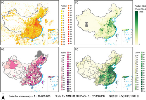
From Figure 1(a), the classified Tencent positioning values can reflect well the characteristics of population density of China (Ge and Feng 2010), where the population densities become denser from the Northwest to the Southeast, and as populations tend to cluster along rivers and coastlines. For example, the Yellow River that is located in North China makes this area dense, while the regions located at Hunagand Yangtze River Delta and Pearl River Delta also attract more settlers. The average Tencent Population Density derived from the Tencent positioning data has been shown to exhibit a simple linear correlation with static census population density (Zheng and Zhang 2020). Thus, we build a simple linear regression model for the two density distributions, which lead to converting TPD to a real population density.

Thus, we unify the two density distributions to a county level. In terms of the TPD distribution at each hourly time, we count the people number in each administrative unit by summing all the values at all points in the unit, then divided by the area of the unit, to get the TPD at the county level. During the study period, there are $145\mathrm{day}\times 24\mathrm{hour}=3480\mathrm{hour}$ Tencent Population Density. Because the EPD is static, we compute the average of the 3480 distributions to obtain the Average Tencent Population Density (ATPD), which is shown in Figure 1(c). Note that in Figure 1(c), the tiny values (the density is very small), e.g. Hegang city in the north of China, are not displayed in the figure. While in Figure 1(d), the null values, for example, Hong Kong, Macao and Taiwan, are excluded in our study. Then, in terms of the EPD, we compute the average value for each administrative unit, then the distribution that has the same spatial resolution as ATPD is plotted in Figure 1(d).

A simple linear regression of the two density distributions is performed, where the results are reported in Section 4.1.

3.1.2 Panel data setup

To detect how dynamic population density changes can affect COVID-19 transmission in time and space, we set the new confirmed case number, new death case number in a day as the dependent variables in the regression, respectively. Because the interval – time from illness onset in a primary case (infector) to illness onset in a secondary case (infectee) of COVID-19 has been estimated to be 4.6 days (Nishiura, Linton, and Akhmetzhanov 2020), while a 14-day delay is the maximum incubation period of the virus (Backer, Klinkenberg, and Wallinga 2020), in this study, the situations of a 5 days lag (≈ 4.6 days) and a 14 day lag of COVID-19 new confirmed and death cases are also considered.

Other supplementary factors that may impact the transmission of COVID-19 are set as the independent variables as well. The reasons are as follows.

Socioeconomic: Age is associated with community-level vulnerability (Andersen et al. 2021). Groups considered to be high-risk include older adults and those with underlying medical conditions, such as obesity, diabetes, and heart disease (Centers for Disease Control and Prevention (CDC) 2020). Thus, we take the number of people whose age is over 65 (the variable has been named as AO), and the Elderly dependency ratio (ER) of each province into consideration. Further, hospital bed number (BN) is also a key impact as more beds in a hospital means a better chance of survival (Mollalo, Vahedi, and Rivera 2020).

The study (Mollalo, Vahedi, and Rivera 2020) found that place-based factors such as median household income, percentage of nurse practitioners, can help explain the significant variations in COVID-19 incidence. Other adverse socioeconomic factors, such as poverty and unemployment, are likely to cause negative health consequences as well (Sun, Hu, and Xie 2021). However, the Chinese government put in place nationwide aid (medicine, nurses, and doctors) against COVID-19, e.g. Hubei’s battle (XINHUANET 2021), while the Chinese authorities regulated that all COVID-19 patients would have their medical expenses fully covered by social health insurance and public finance (World Economic Forum (WEF) 2021). Thus, medical insurance, poverty, and unemployment, percentage of nurse practitioners would not be regarded as the key factors in our study.

Environmental factors: Average and minimum temperature were significantly associated with the COVID-19 pandemic (Bashir et al. 2020; Chen et al. 2020a). Further, humidity also plays a significant role in the seasonal spread of coronaviruses (Sajadi et al. 2020; Poole 2020). Thus, in terms of the weather conditions, we consider temperature (TP) and dew point (DP) which plays the same role with relative humidity as the key environment factors for COVID-19 transmission.

Air pollution plays key role in the influence of human health (Zhang et al. 2020a; Zhang, Rui, and Fan 2018). Previous studies have suggested that ambient air pollutants are risk factors for respiratory infection by carrying microorganisms to make pathogens more invasive in humans, affecting the body’s immunity to make people more susceptible to pathogens (Becker and Soukup 1999; Cai et al. 2007; Horne et al. 2018; Xie et al. 2019; Zhu et al. 2020). Since COVID-19 is a respiratory disease, SARS-CoV-2 could remain viable in aerosols for hours (Van Doremalen et al. 2020). A positive relationship between PM_2.5, PM₁₀, CO, NO₂ and O₃, and COVID-19 transmissions exists (Zhu et al. 2020). Thus, in terms of the air quality factors, AQI with six main air pollutants should also be considered.

However, among the independent variables above, some of them might be highly correlated, which can cause multicollinearity in regression (Alin 2010), for example, AQI is computed by other 6 pollutants. Thus, by following the study (Hu et al. 2021), Variance Inflation Factor (VIF) that can measure how much the variance of regression coefficient is inflated due to multicollinearity is used to exclude the redundancy of the independent variables (VIF1 >10 is used as the cut score (James et al. 2013)). The comparison of the selection of the variables before and after the VIF analysis is reported in Appendix 1. The determining variables definition, resources, and summary descriptions of the dataset are illustrated in Table 1. In the last part of the paper, we called different models based on the dependent variables names, for example, when the dependent variable is NC by using a Spatial Durbin Model (SDM), the model is called NC-SDM.

Table 1. Variable definition, source, and statistic description

Domain	Variable	Description	Source	Mean	Std.	Obs.
Dependent variable
Confirmed Case	NC	New confirmed case number of the day	Bao et al. (Bao, Lin, and Zhou 2020) gathered from the National, Provincial and Autonomous Region’s Health Commission	1.54	67.66	52,780
	NC_Lag5	New confirmed case number lagging 5 days		1.54	67.66	52,780
	NC_Lag14	New confirmed case number lagging 14 days		1.54	67.66	52,780
Death Case	ND	New death case number		0.06	2.00	52,780
	ND_Lag5	New death case number lagging 5 days		0.06	2.00	52,780
	ND_Lag14	New death case number lagging 14 days		0.06	2.00	52,780
Independent variable
People Activity	PD	Tencent population density	Tencent Positioning Data Platform (2020)	$2.83\times {10}^{54}$	$4.59\times {10}^{56}$	52,780
	NPD	New Tencent population density, $\mathit{NPD}=ln\left(\mathit{PD}+1\right)$		54.39	20.54	52,780
Socioeconomic	BN	Hospital beds number per thousand people	China Health Statistics Yearbook 2020 (2021)	6.32	0.83	52,780
	AO	The number of people whose age are over 65		11.19	2.50	52,780
Environmental (Air Quality)	PM25	Average PM2.5 concentration (μg/m^3) in the day.	National Urban Air Quality Real Time Release Platform (2021)	40.22	32.67	52,780
	PM10	Average PM10 concentration (μg/m^3) in the day.		64.00	61.48	52,780
	SO2	Average SO2 concentration (μg/m^3) in the day.		10.13	7.07	52,780
	CO	Average CO concentration (μg/m^3) in the day.		0.76	0.37	52,780
	NO2	Average NO2 concentration (μg/m^3) in the day.		23.46	13.59	52,780
	O3	Average O3 concentration (μg/m^3) in the day.		47.86	20.53	52,780
Environmental (Weather Condition)	TP	Average temperature (°C) in the day.	NOAA National Centers for Environmental Information (2020)	7.71	8.67	52,780
	DP	Average dew point (°C) in the day.		1.97	8.35	52,780

Note: Std. refers to standard deviation. Obs. refers to the number of observations.

The basic data structure is determined as:

• Temporal resolutions: daily.

• Temporal period: 1 December 2019 to 23 April 2020 (145 days).

• Spatial resolutions: county-level administrative unit: on average this area is an average size of 26,000 km² in China. N.B. In other countries, this size can vary and counties can be referred to by other names, such as local government areas (Australia), shires (UK), municipal government (Canada).

• Spatial region: China’s mainland (including 364 county-level cities).

• Variables: six dependent variables and 11 independent variables (no missing values). Note that the variable PD in Table 1 is not used to build a model.

3.2 Model

The transmission of COVID-19 over China is not independent, for example, the confirmed or death case number of a city might be impacted by the case numbers of contiguous cities. Thus, ignoring the spatial correlation associated with cases of COVID-19 flow, may lead to an erroneous model setting. Based on this, this paper selects the spatial panel data analysis technology that takes the spatial correlation of cases of COVID-19 (including both confirmed cases and death cases) into account, to investigate its relationship to dynamic population density changes. At the same time, the direct and indirect effects are computed using the spatial panel data model. When applying a spatial panel data model, a spatial matrix is necessary. Thus, in this section, we first introduce the spatial matrix, then the spatial penal data model is proposed. Third, the special outputs of the model, that is, direct effect and spatial spillover effect, are defined.

3.2.1 Spatial weights matrix

The formula of a spatial weights matrix $\mathit{W}$ is given in Equation (1)(1) $\begin{array}{c}\mathit{W}=\left[\begin{array}{ccc}\begin{array}{cc}{w}_{11}& w_{12}\\ w_{21}& w_{22}\end{array}& \cdots & \begin{array}{c}{w}_{1\mathit{n}}\\ w_{2\mathit{n}}\end{array}\\ ⋮& \ddots & ⋮\\ \begin{array}{cc}{w}_{\mathit{n}1}& w_{\mathit{n}2}\end{array}& \cdots & w_{\mathit{nn}}\end{array}\right]\end{array}$(1) . Supposing there are $\mathit{n}$ spatial objectives, while $\mathit{w}$ is the weight value between every two spatial objectives. For example, $w_{13}$ is the weight value of the first and the third objectives.

(1) $\begin{array}{c}\mathit{W}=\left[\begin{array}{ccc}\begin{array}{cc}{w}_{11}& w_{12}\\ w_{21}& w_{22}\end{array}& \cdots & \begin{array}{c}{w}_{1\mathit{n}}\\ w_{2\mathit{n}}\end{array}\\ ⋮& \ddots & ⋮\\ \begin{array}{cc}{w}_{\mathit{n}1}& w_{\mathit{n}2}\end{array}& \cdots & w_{\mathit{nn}}\end{array}\right]\end{array}$(1)

There are two common weight values, which can construct two kinds of spatial weights matrix. A spatial contiguity matrix is defined if the two spatial objectives, for example, two counties are adjacent, the $\mathit{w}$ of them is set as 1. But, if they have no adjacency, the value is 0 (Equation (2)(2) $w_{\mathit{ij}}=\left\{\begin{array}{c}1,\mathit{i}\mathrm{and}\mathit{j}\mathrm{are}\mathrm{are}\mathrm{neighbors}\\ 0,\mathit{i}\mathrm{and}\mathit{j}\mathrm{are}\mathrm{are}\mathrm{not}\mathrm{neighbors}\end{array}\right.$(2) ).

(2) $w_{\mathit{ij}}=\left\{\begin{array}{c}1,\mathit{i}\mathrm{and}\mathit{j}\mathrm{are}\mathrm{are}\mathrm{neighbors}\\ 0,\mathit{i}\mathrm{and}\mathit{j}\mathrm{are}\mathrm{are}\mathrm{not}\mathrm{neighbors}\end{array}\right.$(2)

Another matrix is a spatial inverse distance matrix, where the $\mathit{w}$ between the objective $\mathit{i}$ and $\mathit{j}$ is $1/d_{\mathit{ij}}$, as shown in Equation (3)(3) $\begin{array}{c}{w}_{\mathit{ij}}=\frac{1}{{\mathit{d}}_{\mathit{ij}}}\end{array}$(3) . To be specific, $\mathit{w}$ is calculated as the inverse distance between the geographical centers of county $\mathit{i}$ and $\mathit{j}$.

(3) $\begin{array}{c}{w}_{\mathit{ij}}=\frac{1}{{\mathit{d}}_{\mathit{ij}}}\end{array}$(3)

A spatial contiguity matrix highlights the impact from the closest neighbors, while a spatial inverse distance matrix underlines the effect that this diminishes as distance increases. The two spatial matrixes are simultaneously used to test the robustness of the spatial regression model. Therefore, we use both matrixes as inputs to our spatial models.

3.2.2 Spatial dependency examination

Before using a spatial model, Moran’s I spatial statistic is needed to test whether spatial dependencies (also well known as spatial autocorrelation) in the dependent variables exist (Kang et al. 2020; Li, Calder, and Cressie 2007). In this study, we examine the monthly spatial dependency for COVID-19 related dependent variables by computing the global Moran’ I (Goodchild 1986; Saffary et al. 2020). A positive global Moran’s I value with statistical significance indicates spatial clustering, while a significant and negative Moran’s I value indicates spatial dispersion across the study region.

However, because the panel structure of the dataset is applied in our study, where both dependent and independent variables are continuous in both time and space, the daily or monthly Moran’s Is are hard to examine the spatial dependency for the panel data structure, which can be alternatively expressed in several other ways, for example, spatial lag effect (Elhorst 2001). Thus, another index such as a coefficient of the spatial lag effect in a model is needed and proposed as a further test. We further use the coefficient $\mathit{\delta }$ in Equation (4)(4) $Y_{\mathit{it}}={\beta }_0+\mathit{\delta }\mathit{W}{Y}_{\mathit{it}}+{\beta }_1\mathit{lnP}{D}_{\mathit{it}}+{\beta }_2\mathit{B}{N}_{\mathit{it}}+{\beta }_3\mathit{A}{O}_{\mathit{it}}+{\alpha }^T\mathit{A}\mathit{QT}\text{}{\text{}}_{\mathit{it}}+{\gamma }^T\mathit{W}\mathit{CT}\text{}{\text{}}_{\mathit{it}}+{\theta }_1\mathit{W}\mathit{lnP}{D}_{\mathit{it}}+{\theta }_2\mathit{W}\mathit{B}{N}_{\mathit{it}}+{\theta }_3\mathit{W}\mathit{A}{O}_{\mathit{it}}+{\rho }^T\mathit{WA}\mathit{QT}\text{}{\text{}}_{\mathit{it}}+{\vartheta }^T\mathit{WW}{C}_{\mathit{it}}\mathit{T}+{\epsilon }_{\mathit{it}}$(4) to illustrate this point (LeSage and Pace 2009) in the next section.

3.2.3 SDM

There are two common spatial panel data models, a Spatial Autoregressive Model (SAR) (Griffith 1988), which only considers the spatial dependent variables, and a Spatial Error Model (SEM) (Anselin and Griffith 1988), which contains only the autocorrelation of spatial error terms. However, the conduction of spatial effects including spatial heterogeneity and spatial dependence may occur simultaneously and represented as the variation of the error term caused by the spatial lag of the dependent variable and random impact. Thus, a Spatial Durbin Model (SDM) was used (LeSage and Pace 2009) to consider the spatial interaction, for example, a dependent variable in one city is not only influenced by the independent variables in the same city, but also by both dependent and independent variables in one or more contiguous cities.

This study mainly uses SDMs to detect the quantitative relationship between the confirmed or death case number and dynamic population density changes. Nevertheless, because different spatial panel data models are proposed for different purposes, to obtain the best fitted spatial panel data model, we present a process to pretest the robustness (prerobustness test) of the SDMs: first, building SDMs for the datasets, which have been described in Section 3.1.2. Second, testing if the SDMs could be simplified to SARs. Third, testing if the SDMs could be transferred to SEMs. Finally, using the Hausman test to determine if we use a Fixed Effect (FE) or a Random Effect (RF) to the SDMs. The specific steps are shown below.

First, an SDE model could be built as Equation (4)(4) $Y_{\mathit{it}}={\beta }_0+\mathit{\delta }\mathit{W}{Y}_{\mathit{it}}+{\beta }_1\mathit{lnP}{D}_{\mathit{it}}+{\beta }_2\mathit{B}{N}_{\mathit{it}}+{\beta }_3\mathit{A}{O}_{\mathit{it}}+{\alpha }^T\mathit{A}\mathit{QT}\text{}{\text{}}_{\mathit{it}}+{\gamma }^T\mathit{W}\mathit{CT}\text{}{\text{}}_{\mathit{it}}+{\theta }_1\mathit{W}\mathit{lnP}{D}_{\mathit{it}}+{\theta }_2\mathit{W}\mathit{B}{N}_{\mathit{it}}+{\theta }_3\mathit{W}\mathit{A}{O}_{\mathit{it}}+{\rho }^T\mathit{WA}\mathit{QT}\text{}{\text{}}_{\mathit{it}}+{\vartheta }^T\mathit{WW}{C}_{\mathit{it}}\mathit{T}+{\epsilon }_{\mathit{it}}$(4) ,

(4) $Y_{\mathit{it}}={\beta }_0+\mathit{\delta }\mathit{W}{Y}_{\mathit{it}}+{\beta }_1\mathit{lnP}{D}_{\mathit{it}}+{\beta }_2\mathit{B}{N}_{\mathit{it}}+{\beta }_3\mathit{A}{O}_{\mathit{it}}+{\alpha }^T\mathit{A}\mathit{QT}\text{}{\text{}}_{\mathit{it}}+{\gamma }^T\mathit{W}\mathit{CT}\text{}{\text{}}_{\mathit{it}}+{\theta }_1\mathit{W}\mathit{lnP}{D}_{\mathit{it}}+{\theta }_2\mathit{W}\mathit{B}{N}_{\mathit{it}}+{\theta }_3\mathit{W}\mathit{A}{O}_{\mathit{it}}+{\rho }^T\mathit{WA}\mathit{QT}\text{}{\text{}}_{\mathit{it}}+{\vartheta }^T\mathit{WW}{C}_{\mathit{it}}\mathit{T}+{\epsilon }_{\mathit{it}}$(4)

$\mathit{A}{Q}_{\mathit{it}}={\left(\mathit{PM}{25}_{\mathit{it}},\mathit{PM}{10}_{\mathit{it}},\mathit{SO}{2}_{\mathit{it}},\mathit{C}{O}_{\mathit{it}},\mathit{NO}{2}_{\mathit{it}},\mathit{O}{3}_{\mathit{it}}\right)}^{\mathit{T}},\mathit{\alpha }={\left({\alpha }_1,{\alpha }_2,\dots ,{\alpha }_6\right)}^{\mathit{T}},\mathit{\rho }={\left({\rho }_1,{\rho }_2,\dots ,{\rho }_6\right)}^{\mathit{T}}$

$\mathit{W}{C}_{\mathit{it}}=\left(\mathit{T}{P}_{\mathit{it}},\mathit{D}{P}_{\mathit{it}}\right)\mathit{T},\mathit{\gamma }=\left({\gamma }_1,{\gamma }_2\right)\mathit{T},\mathit{\vartheta }=\left({\vartheta }_1,{\vartheta }_2\right)\mathit{T}$

The variables have been defined in Table 1, while the correlation coefficients of the variables could be represented by ${\beta }_1\sim {\beta }_4,\mathit{\alpha },\mathit{\rho },{\theta }_1\sim {\theta }_4,\mathit{\gamma },\mathit{\vartheta }$.

Second, when the spatial interaction examined by the SDM model does not exist and there is only a one-way spatial correlation between regions, which means ${\theta }_i=0\left(\mathit{i}=1,2,3\right)$, ${\rho }_i=0$ $\left(\mathit{i}=1,2,\dots ,7\right)$, and ${\vartheta }_i=0$ $\left(\mathit{i}=1,2\right)$, the model changes to a Spatial Autoregressive Model (SAR):

(5) $Y_{\mathit{it}}={\beta }_0+\mathit{\delta }\mathit{W}{Y}_{\mathit{it}}+{\beta }_1\mathit{lnP}{D}_{\mathit{it}}+{\beta }_2\mathit{B}{N}_{\mathit{it}}+{\beta }_3\mathit{A}{O}_{\mathit{it}}+{\alpha }^T\mathit{A}\mathit{Q}\mathit{T}{\text{}}_{\mathit{it}}+{\gamma }^T\mathit{W}\mathit{C}\mathit{T}\text{}{\text{}}_{\mathit{it}}+{\epsilon }_{\mathit{it}}$(5)

$\mathit{A}{Q}_{\mathit{it}}={\left(\mathit{PM}{25}_{\mathit{it}},\mathit{PM}{10}_{\mathit{it}},\mathit{SO}{2}_{\mathit{it}},\mathit{C}{O}_{\mathit{it}},\mathit{NO}{2}_{\mathit{it}},\mathit{O}{3}_{\mathit{it}}\right)}^{\mathit{T}},\mathit{\alpha }={\left({\alpha }_1,{\alpha }_2,\dots ,{\alpha }_6\right)}^{\mathit{T}}$

$\mathit{W}{C}_{\mathit{it}}={\left(\mathit{T}{\mathit{P}}_{\mathit{it}},\mathit{D}{P}_{\mathit{it}}\right)}^{\mathit{T}},\mathit{\gamma }={\left({\gamma }_1,{\gamma }_2\right)}^{\mathit{T}}$

Thus, we only test if the ${\theta }_1\sim {\theta }_4,\mathit{\gamma },\mathit{\vartheta }$ in Equation (4)(4) $Y_{\mathit{it}}={\beta }_0+\mathit{\delta }\mathit{W}{Y}_{\mathit{it}}+{\beta }_1\mathit{lnP}{D}_{\mathit{it}}+{\beta }_2\mathit{B}{N}_{\mathit{it}}+{\beta }_3\mathit{A}{O}_{\mathit{it}}+{\alpha }^T\mathit{A}\mathit{QT}\text{}{\text{}}_{\mathit{it}}+{\gamma }^T\mathit{W}\mathit{CT}\text{}{\text{}}_{\mathit{it}}+{\theta }_1\mathit{W}\mathit{lnP}{D}_{\mathit{it}}+{\theta }_2\mathit{W}\mathit{B}{N}_{\mathit{it}}+{\theta }_3\mathit{W}\mathit{A}{O}_{\mathit{it}}+{\rho }^T\mathit{WA}\mathit{QT}\text{}{\text{}}_{\mathit{it}}+{\vartheta }^T\mathit{WW}{C}_{\mathit{it}}\mathit{T}+{\epsilon }_{\mathit{it}}$(4) equal zero, to determine if the SDM could be simplified to Equation (5)(5) $Y_{\mathit{it}}={\beta }_0+\mathit{\delta }\mathit{W}{Y}_{\mathit{it}}+{\beta }_1\mathit{lnP}{D}_{\mathit{it}}+{\beta }_2\mathit{B}{N}_{\mathit{it}}+{\beta }_3\mathit{A}{O}_{\mathit{it}}+{\alpha }^T\mathit{A}\mathit{Q}\mathit{T}{\text{}}_{\mathit{it}}+{\gamma }^T\mathit{W}\mathit{C}\mathit{T}\text{}{\text{}}_{\mathit{it}}+{\epsilon }_{\mathit{it}}$(5) (SAR), which is set as Hypothesis 0. If the hypothesis has been rejected (p < 0.5), the SDM cannot be transferred to a SAR.

Third, when the coefficient of spatial interaction ${\theta }_i$, the spatial lag coefficient $\mathit{\delta }$ and the regression coefficient ${\beta }_i$ of the dependent variable meet the requirements of ${\theta }_i=-\mathit{\delta }{\beta }_i$, $\mathit{\gamma }=-\mathit{\delta \alpha }$, $\mathit{\vartheta }=-\mathit{\delta \rho }$, then the model changes to a Spatial Error Model (SEM):

(6) $\begin{array}{rl}& Y_{\mathit{it}}={\beta }_0+{\beta }_{1}ln\mathit{P}{D}_{\mathit{it}}+{\beta }_2\mathit{B}{N}_{\mathit{it}}+{\beta }_3\mathit{A}{O}_{\mathit{it}}+{\alpha }^T{\mathit{A}Q}_{it}^T\\ & +\mathit{\gamma }{ }^T{\mathit{WC}}^T{}_{\mathit{it}}+{\mu }_{\mathit{it}},\\ & {\mu }_{\mathit{it}}=\mathit{\lambda }\mathbf{W}{\mu }_t+{\epsilon }_{\mathit{it}}\\ & {\mathit{A}\mathit{Q}}_{\mathit{it}}={\left(\mathit{PM}{25}_{\mathit{it}},\mathit{PM}{10}_{\mathit{it}},\mathit{SO}{2}_{\mathit{it}},\mathit{C}{O}_{\mathit{it}},\mathit{NO}{2}_{\mathit{it}},\mathit{O}{3}_{\mathit{it}}\right)}^{\mathit{T}},\\ & \mathit{\alpha }={\left({\alpha }_1,{\alpha }_2,\dots ,{\alpha }_6\right)}^{\mathit{T}}\text{break}{\mathit{W}\mathit{C}}_{\mathit{it}}={\left(\mathit{T}{\mathit{P}}_{\mathit{it}},\mathit{D}{P}_{\mathit{it}}\right)}^{\mathit{T}},\\ & \mathit{\gamma }={\left({\gamma }_1,{\gamma }_2\right)}^{\mathit{T}}\end{array}$(6)

Thus, to set a Hypothesis 0 based on a nonlinear test, if the hypothesis has been rejected (p < 0.05), the SDM could not be transferred to an SEM (Equation (6)(6) $\begin{array}{rl}& Y_{\mathit{it}}={\beta }_0+{\beta }_{1}ln\mathit{P}{D}_{\mathit{it}}+{\beta }_2\mathit{B}{N}_{\mathit{it}}+{\beta }_3\mathit{A}{O}_{\mathit{it}}+{\alpha }^T{\mathit{A}Q}_{it}^T\\ & +\mathit{\gamma }{ }^T{\mathit{WC}}^T{}_{\mathit{it}}+{\mu }_{\mathit{it}},\\ & {\mu }_{\mathit{it}}=\mathit{\lambda }\mathbf{W}{\mu }_t+{\epsilon }_{\mathit{it}}\\ & {\mathit{A}\mathit{Q}}_{\mathit{it}}={\left(\mathit{PM}{25}_{\mathit{it}},\mathit{PM}{10}_{\mathit{it}},\mathit{SO}{2}_{\mathit{it}},\mathit{C}{O}_{\mathit{it}},\mathit{NO}{2}_{\mathit{it}},\mathit{O}{3}_{\mathit{it}}\right)}^{\mathit{T}},\\ & \mathit{\alpha }={\left({\alpha }_1,{\alpha }_2,\dots ,{\alpha }_6\right)}^{\mathit{T}}\text{break}{\mathit{W}\mathit{C}}_{\mathit{it}}={\left(\mathit{T}{\mathit{P}}_{\mathit{it}},\mathit{D}{P}_{\mathit{it}}\right)}^{\mathit{T}},\\ & \mathit{\gamma }={\left({\gamma }_1,{\gamma }_2\right)}^{\mathit{T}}\end{array}$(6) ).

Finally, we consider using a FE or RE estimator to perform the SDMs. Because in Equation (4)(4) $Y_{\mathit{it}}={\beta }_0+\mathit{\delta }\mathit{W}{Y}_{\mathit{it}}+{\beta }_1\mathit{lnP}{D}_{\mathit{it}}+{\beta }_2\mathit{B}{N}_{\mathit{it}}+{\beta }_3\mathit{A}{O}_{\mathit{it}}+{\alpha }^T\mathit{A}\mathit{QT}\text{}{\text{}}_{\mathit{it}}+{\gamma }^T\mathit{W}\mathit{CT}\text{}{\text{}}_{\mathit{it}}+{\theta }_1\mathit{W}\mathit{lnP}{D}_{\mathit{it}}+{\theta }_2\mathit{W}\mathit{B}{N}_{\mathit{it}}+{\theta }_3\mathit{W}\mathit{A}{O}_{\mathit{it}}+{\rho }^T\mathit{WA}\mathit{QT}\text{}{\text{}}_{\mathit{it}}+{\vartheta }^T\mathit{WW}{C}_{\mathit{it}}\mathit{T}+{\epsilon }_{\mathit{it}}$(4) , ${\epsilon }_{\mathit{it}}={\lambda }_i+{\upsilon }_{\mathit{it}}$, for random effects, we assume the ${\lambda }_i$ are part of the composite error term ${\epsilon }_{\mathit{it}}$. To construct an efficient estimator, we need to evaluate the structure of the error and then apply an appropriate generalized least squares estimator to find an efficient estimator.

The Random Effects estimator has the standard generalized least squares form summed over all individuals in the dataset:

(7) ${\widehat{\beta }}_{\mathit{RE}}={\left[{\displaystyle \sum _{\mathit{i}=1}^N\left(X_i^T{\Omega }^{-1}{X}_i\right)}\right]}^{-1}{\displaystyle \sum _{\mathit{i}=1}^N\left(X_i^T{\Omega }^{-1}{Y}_i\right)},\mathit{\Omega }={\sigma }_u^2\mathit{I}+{\sigma }_{\lambda }^2\mathit{e}{e}^T$(7)

In Equation (7)(7) ${\widehat{\beta }}_{\mathit{RE}}={\left[{\displaystyle \sum _{\mathit{i}=1}^N\left(X_i^T{\Omega }^{-1}{X}_i\right)}\right]}^{-1}{\displaystyle \sum _{\mathit{i}=1}^N\left(X_i^T{\Omega }^{-1}{Y}_i\right)},\mathit{\Omega }={\sigma }_u^2\mathit{I}+{\sigma }_{\lambda }^2\mathit{e}{e}^T$(7) , ${\mathit{e}}^T=\left(1,1,1\dots ,1\right)$ is a unit vector of size $\mathit{T}$.

The fixed effects estimator can be written in:

(8) ${\hat{\beta }}_{\mathit{FE}}={\left[\sum _{\mathit{i}=1}^T\left(X_i^T\mathit{M}{X}_i\right)\right]}^{-1}\sum _{\mathit{i}=1}^T\left(X_i^T\mathit{M}{Y}_i\right),\mathit{M}=I_T-\frac{1}{T}{\mathit{e}\mathit{e}}^T$(8)

If there is no correlation between regressors and effects, then FE and RE are both consistent, but FE is inefficient. If there is a correlation, FE is consistent and RE is inconsistent. Under the null hypothesis of no correlation, there should be no differences between the estimators. Thus, we follow the process of the Hausman test (Hausman 1978) to determine which effects estimator is better. The covariance of an efficient estimator with its difference from an inefficient estimator should be zero. Under the null hypothesis, we test:

(9) $\mathit{H}={\left({\mathit{\beta }}_{\mathit{RE}}-{\beta }_{\mathit{FE}}\right)}^{\mathit{T}}{\widehat{\Sigma }}^{-1}\left({\beta }_{\mathit{RE}}-{\beta }_{\mathit{FE}}\right)~{\chi }^2\left(\mathit{k}\right)$(9)

If $\mathit{H}$ is significant, we should use the fixed effects estimator. Otherwise, a random-effects estimator is better.

3.2.4 Direct and indirect effects

In a spatial panel data model with the spatial lag term, the influence of the independent variable on the dependent variable cannot be simply represented by the regression coefficient. According to the different scope and objects of spatial effect, LeSage and Pace (LeSage and Pace 2008) divided the influence of independent variables on dependent variables in a spatial panel data model into direct effect, indirect effect (spatial spillover effect). A direct effect reflects the average influence of an independent variable $\mathit{x}$ on $\mathit{y}$ in this region. An indirect effect reflects the average influence of independent variable $\mathit{x}$ on $\mathit{y}$ in other regions. Later, they found that a partial differential method can make up for the shortcomings of the point estimation method in explaining the spatial effect. This more effectively explains the impact of any random impact on each variable, and determines the direct effect and indirect effect of an independent variable on the dependent variable in a spatial econometric model (LeSage and Pace 2009). This further processing is defined below:

First, transferring the general form of an SDM to:

(10) $\left(I_n-\mathit{\delta }\mathit{W}\right)\mathit{Y}={\tau }_n\mathit{\beta }{ }^T{}_0+\mathit{\beta X}+\mathit{\theta }\mathit{W}\mathit{X}+\mathit{\epsilon }$(10)

Second, using the setting below:

(11) $\mathit{P}\left(\mathit{W}\right)={\left(I_n-\mathit{\delta }\mathit{W}\right)}^{-1},Q_m\left(\mathit{W}\right)=\mathit{P}\left(\mathit{W}\right)\cdot \left(I_n{\beta }_m+{\theta }_m\mathit{W}\right)$(11)

Then the formula becomes:

(12) $\mathit{Y}=\sum _{\mathit{m}=1}^k{Q}_m\left(\mathit{W}\right)X_m+\mathit{P}\left(\mathit{W}\right){\tau }_n\mathit{\beta }{{ }^T}_0+\mathit{P}\left(\mathit{W}\right)\mathit{\epsilon }$(12)

which is equal to a matrix form:

(13) $\left[\begin{array}{c}{Y}_1\\ Y_2\\ ⋮\\ Y_n\end{array}\right]=\sum { }_{m=1}^k\left[\begin{array}{ccc}\begin{array}{cc}{\mathit{Q}}_{\mathit{m}}{\left(\mathit{W}\right)}_{\mathbf{11}}& {\mathit{Q}}_{\mathit{m}}{\left(\mathit{W}\right)}_{12}\\ {\mathit{Q}}_{\mathit{m}}{\left(\mathit{W}\right)}_{21}& {\mathit{Q}}_{\mathit{m}}{\left(\mathit{W}\right)}_{22}\end{array}& \cdots & \begin{array}{c}{\mathit{Q}}_{\mathit{m}}{\left(\mathit{W}\right)}_{1\mathit{n}}\\ {\mathit{Q}}_{\mathit{m}}{\left(\mathit{W}\right)}_{21}\end{array}\\ ⋮& \ddots & ⋮\\ \begin{array}{cc}{\mathit{Q}}_{\mathit{m}}{\left(\mathit{W}\right)}_{\left(\mathit{n}-1\right)1}& {\mathit{Q}}_{\mathit{m}}{\left(\mathit{W}\right)}_{\left(\mathit{n}-2\right)2}\\ {\mathit{Q}}_{\mathit{m}}{\left(\mathit{W}\right)}_{\mathit{n}1}& {\mathit{Q}}_{\mathit{m}}{\left(\mathit{W}\right)}_{\mathit{n}2}\end{array}& \cdots & \begin{array}{c}{\mathit{Q}}_{\mathit{m}}{\left(\mathit{W}\right)}_{\left(\mathit{n}-1\right)\mathit{n}}\\ {\mathit{Q}}_{\mathit{m}}{\left(\mathit{W}\right)}_{\mathit{nn}}\end{array}\end{array}\right]\left[\begin{array}{c}\begin{array}{c}\begin{array}{c}{\mathit{X}}_{1\mathit{m}}\\ {\mathit{X}}_{2\mathit{m}}\end{array}\\ ⋮\end{array}\\ {\mathit{X}}_{\mathit{nm}}\end{array}\right]+\mathit{P}(\mathit{W})\left({\tau }_n\mathit{\beta }{ }^{\mathrm{\prime }}{{ }^T}_0+\mathit{\epsilon }\right)$(13)

Within Equation (13)(13) $\left[\begin{array}{c}{Y}_1\\ Y_2\\ ⋮\\ Y_n\end{array}\right]=\sum { }_{m=1}^k\left[\begin{array}{ccc}\begin{array}{cc}{\mathit{Q}}_{\mathit{m}}{\left(\mathit{W}\right)}_{\mathbf{11}}& {\mathit{Q}}_{\mathit{m}}{\left(\mathit{W}\right)}_{12}\\ {\mathit{Q}}_{\mathit{m}}{\left(\mathit{W}\right)}_{21}& {\mathit{Q}}_{\mathit{m}}{\left(\mathit{W}\right)}_{22}\end{array}& \cdots & \begin{array}{c}{\mathit{Q}}_{\mathit{m}}{\left(\mathit{W}\right)}_{1\mathit{n}}\\ {\mathit{Q}}_{\mathit{m}}{\left(\mathit{W}\right)}_{21}\end{array}\\ ⋮& \ddots & ⋮\\ \begin{array}{cc}{\mathit{Q}}_{\mathit{m}}{\left(\mathit{W}\right)}_{\left(\mathit{n}-1\right)1}& {\mathit{Q}}_{\mathit{m}}{\left(\mathit{W}\right)}_{\left(\mathit{n}-2\right)2}\\ {\mathit{Q}}_{\mathit{m}}{\left(\mathit{W}\right)}_{\mathit{n}1}& {\mathit{Q}}_{\mathit{m}}{\left(\mathit{W}\right)}_{\mathit{n}2}\end{array}& \cdots & \begin{array}{c}{\mathit{Q}}_{\mathit{m}}{\left(\mathit{W}\right)}_{\left(\mathit{n}-1\right)\mathit{n}}\\ {\mathit{Q}}_{\mathit{m}}{\left(\mathit{W}\right)}_{\mathit{nn}}\end{array}\end{array}\right]\left[\begin{array}{c}\begin{array}{c}\begin{array}{c}{\mathit{X}}_{1\mathit{m}}\\ {\mathit{X}}_{2\mathit{m}}\end{array}\\ ⋮\end{array}\\ {\mathit{X}}_{\mathit{nm}}\end{array}\right]+\mathit{P}(\mathit{W})\left({\tau }_n\mathit{\beta }{ }^{\mathrm{\prime }}{{ }^T}_0+\mathit{\epsilon }\right)$(13) , $\mathit{m}=1,2,\dots ,\mathit{k}$, which represents the $\mathit{k}$-th independent variable. The right part of the equal sign is a partial differential matrix, where the diagonal elements reflect the average influence of the change of $X_{\mathit{ik}}$ variable in a specific space unit on the dependent variable of the unit, namely direct effect. The non-diagonal elements represent the average influence of the change of $X_{\mathit{ik}}$ variable in a specific space unit on the dependent variable of other space units, namely the indirect effect (also well-known as space spillover effect). Equations (14)(14) $\mathit{direct}=\frac{\partial Y_i}{\partial X_{\mathit{im}}}={\theta }_m\mathit{W}\mathit{ii}$(14) to (15(15) $\mathit{indirect}=\frac{\partial Y_i}{\partial X_{\mathit{jm}}}={\theta }_m\mathit{W}\mathit{ij}$(15) ) give the formulae for direct and indirect effects:

(14) $\mathit{direct}=\frac{\partial Y_i}{\partial X_{\mathit{im}}}={\theta }_m\mathit{W}\mathit{ii}$(14)

(15) $\mathit{indirect}=\frac{\partial Y_i}{\partial X_{\mathit{jm}}}={\theta }_m\mathit{W}\mathit{ij}$(15)

3.3 Validation

To test our results of the estimation in both qualitative and quantitative scales, two validation strategies are proposed.

3.3.1 Validation strategy 1 (VS1): random experiment

Random experiments can solve the potential endogeneity issue brought about by an omitted variable (Berk 1983), which has been widely used in the cross-validation of panel data models (Zhang et al. 2021). A ten-fold cross-validation has been conducted in this study. The process is described as below.

Over the study period, we randomly extract 60% samples of data in temporal-continuous days (87 days) for 10 rounds, where each round is regarded as one random experiment, and then build SDE models for 10 rounds. To quantify the reliability of the results, the Reliability Indices (RIs) for both coefficient (${\beta }_1$ in SDE model) and its significance has been defined as below,

(16) $\begin{array}{c}\mathit{R}{I}_{\mathit{coef}.}=\frac{{{\beta }_1}_{\mathit{m}}-{{\beta }_1}_{\mathit{cv}-\mathit{mean}}}{{{\beta }_1}_{\mathit{m}}}\end{array}$(16)

(17) $\begin{array}{c}\mathit{R}{I}_{\mathit{sig}.}=\frac{{\mathrm{N}}_{\mathit{cons}.}}{{\mathrm{N}}_{\mathit{total}}}\end{array}$(17)

where in Equation (16)(16) $\begin{array}{c}\mathit{R}{I}_{\mathit{coef}.}=\frac{{{\beta }_1}_{\mathit{m}}-{{\beta }_1}_{\mathit{cv}-\mathit{mean}}}{{{\beta }_1}_{\mathit{m}}}\end{array}$(16) , RI of the coefficient is represented by $\mathit{R}{I}_{\mathit{coef}.}$, and ${{\beta }_1}_{\mathit{m}}$ indicates the ${\beta }_1$ in the main result, while ${{\beta }_1}_{\mathit{cv}-\mathit{mean}}$ indicates the mean ${\beta }_1$ values over the 10-round random experiments. Similarly, RI of the significance is represented by $\mathit{R}{I}_{\mathit{sig}.}$, and ${\mathrm{N}}_{\mathit{cons}.}$ indicates the number of times this is consistent with the main results, while ${\mathrm{N}}_{\mathit{total}}$ means the total number of the random experiments, which is 10 in this study.

These parameters can provide key references to the reliability of the SDE models, which also improve the evaluability of the study.

3.3.2 Validation strategy 2 (VS2): independent dataset test

To further test the robustness of the results of this study, VS2 uses an independent dataset to validate the results.

As another popular volunteer GIS data, Baidu migration data (Baidu 2020), that is also widely used in GIS-oriented work (Wei and Wang 2020; Zhan et al. 2020; Chen et al. 2017), can be applied as an independent test. The migration of people from city to city throughout the country was recorded as location-based data using the search engine Baidu. Every city is represented using two vectors. The first one describes the situation of access to a city, called the Migrate In Index. The other index reflects the population movement from this city to another one, called the Migrate Out Index). The two indices are used on a daily dataset. These indices were only indicative of the relative volume of movement of people from one city to another. Thus, the migration strengths of cities, serve as indicative measures of the human transfer volume moving in and out of administrative units (Zhan et al. 2020).

However, the difference between the Migrate In Index and Migrate Out Index can reflect the population Net Increase (NI) of an administrative unit in a day, which has the same effect to measure the people’s density change at a spatiotemporal scale, qualitatively. Thus, the Baidu migration NI (BMNI) can validate the main results of this study in a qualitative way.

The available historical Baidu migration data cover the days from 10 January 2020 to 15 March 2020 (65 days), we only build the model between the independent variables and the COVID-19 cases (confirmed and death) on the day and after 5 days (if we consider after 14 days, the period would be reduced to 51 days, equal to losing more than 20% of samples), so we extract the panel dataset corresponding to the period on the day and after 5 day’s situation of COVID-19. And then NPD is replaced by BMNI to construct the SDE models with the same steps.

4. Results

4.1 Relationship between Tencent and real population densities

We find there is a simple linear relationship between the logarithms of the ATPD and EPD in 2015, where the function is statistically significant (p < 0.001, R² = 0.93). Figure 2 shows the details of the regression.

Figure 2. Simple linear regression between ATPD and EPD.

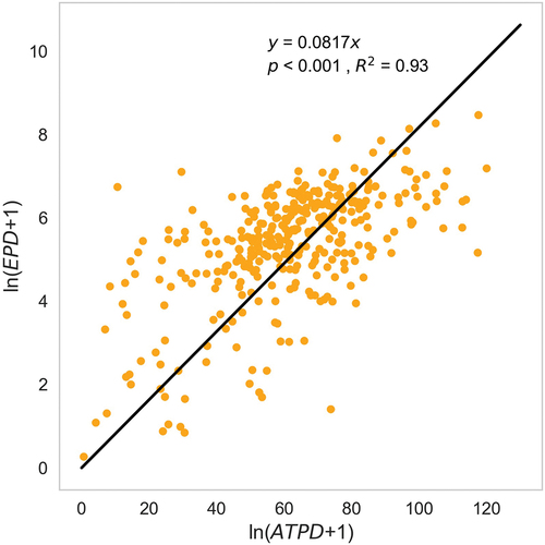
The function could be represented by Equation (18)(18) $ln\left(\mathit{ATPD}+1\right)=0.0817\times ln\left(\mathit{EPD}+1\right)$(18) , where the coefficient is 0.0817:

(18) $ln\left(\mathit{ATPD}+1\right)=0.0817\times ln\left(\mathit{EPD}+1\right)$(18)

According to the above equation, the EPD could be computed by Equation (19)(19) $\mathit{EPD}=e^{\frac{ln\left(\mathit{ATPD}+1\right)}{0.0817}}-1$(19) :

(19) $\mathit{EPD}=e^{\frac{ln\left(\mathit{ATPD}+1\right)}{0.0817}}-1$(19)

Based on this, the relationship between the Tencent population density with higher temporal resolution such as hourly and daily (defined as New PD, NPD, Table 1), and estimated dynamic population density (EDPD) could be represented by Equation (20)(20) $\mathit{EDPD}=e^{\frac{ln\left(\mathit{PD}+1\right)}{0.0817}}-1=e^{\frac{\mathit{NPD}}{0.0817}}-1$(20) :

(20) $\mathit{EDPD}=e^{\frac{ln\left(\mathit{PD}+1\right)}{0.0817}}-1=e^{\frac{\mathit{NPD}}{0.0817}}-1$(20)

An EDPD could be computed by NPD, which means the quantitative impact of NPD on the transmission of COVID-19 could be transferred to the quantitative impact of estimated dynamic population density on the transmission.

4.2 Spatial dependency examination

The monthly global Moran’s I has been shown in Table 2, where the values that are not significant have been excluded. The remaining values are all significant, positive, which means the COVID-19 related variables have a high spatial dependency during the specific months.

Table 2. Monthly global Moran’s I for dependent variables

	NC	NC_Lag5	NC_Lag14	ND	ND_Lag5	ND_Lag14
Dec. 2019	.	.	.	.	.	.
Jan. 2020	0.130	0.099	0.045	0.035	0.037	0.028
Feb. 2020	0.031	0.021	0.010	0.024	0.023	0.023
Mar. 2020	.	.	.	0.022	0.014	0.008
Apr. 2020	0.129	0.168	0.180	.	.	.

Note: The insignificant values have been shown as “.”.

Note, at the start of the pandemic of COVID-19, e.g. Dec. 2019, the cases appeared sparsely distributed among the cities in China, which causes the Moran’s Is to be not significant. However, overall there is a high spatial dependency of the COVID-19 related variables (at least 60% are significant positive), which is consistent with other related research that focuses on China (Kang et al. 2020; Zhang et al. 2020c) and this is also found in other countries (Bag et al. 2020; Shariati et al. 2020).

4.3 Model prerobustness test

Table 3 shows the results of the decision if an SDM should be simplified to a SAR or SEM and Hausman test. According to Section 3.2.3, because all the p-values in the column SAR and SEM are less than 0.01, which means the original hypothesis is rejected. Thus, the SDMs should not be simplified to SARs or SEMs, which means the two kinds of spatial transmission mechanisms in an SDM cannot be ignored. Further, because the Hausman test result (column Hau. p-value) shows that the original hypothesis has not been rejected for each SDM, a random effect (FE) estimator should be selected to perform the SDMs.

Table 3. SDM pre-robustness test and effect selection

Spatial Matrix	Dependent Variable	SAR p-value	SEM p-value	Hau. p-value
Contiguity	NC	< 0.01	< 0.01	0.66
	NC_Lag5	< 0.01	< 0.01	0.74
	NC_Lag14	< 0.01	< 0.01	0.66
	ND	< 0.01	< 0.01	0.56
	ND_Lag5	< 0.01	< 0.01	0.67
	ND_Lag14	< 0.01	< 0.01	0.32
Inverse Distance	NC	< 0.01	< 0.01	0.73
	NC_Lag5	< 0.01	< 0.01	0.80
	NC_Lag14	< 0.01	< 0.01	0.79
	ND	< 0.01	< 0.01	0.93
	ND_Lag5	< 0.01	< 0.01	0.89
	ND_Lag14	< 0.01	< 0.01	0.55

Note: Hau. refers to Hausman test.

4.4 Main results of SDM

After the robust test and Hausman test, an SDM model with a random effect estimator method is determined. The main coefficients of NPD in regression results are shown in Figure 3. Within them, the left 6 bars in the figure show the results using a spatial contiguity matrix, while the right 6 bars illustrate the use of a spatial inverse distance matrix. The full results have been reported in Table A.3 and A.4 in Appendix 2, where the spatial lag coefficient $\mathit{\delta }$ of all 12 SDMs is significantly positive, which means the (lagged) confirmed or death cases of COVID-19 in one administrative unit are impacted by the situation of its neighbor units. Thus, a spatial panel data model is necessary rather than a normal panel data model.

Figure 3. Main coefficients of NPD. (* p < 0.05, ** p < 0.01, *** p < 0.001).

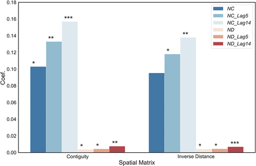
In Figure 3, 12 coefficients are positive while 11 of them is significant except NC by inverse distance matrix is not significant. The coefficients of NPD for confirmed case SDMs (NC, NC_Lag5, NC_Lag14) are higher than the death case SDMs (ND, ND_Lag5, ND_Lag14). Coefficients of both confirmed and death case SDMs for each spatial matrix grow with the increase of lag of days (nolag-lag5-lag14). For the contiguity matrix, the coefficients for SDMs of NC, NC_Lag5, and NC_ Lag14 by the contiguity matrix are 0.103 (p < 0.05), 0.133 (p < 0.01), 0.157 (p < 0.01), while the values for death case are 0.0038 (p < 0.05), 0.004,39 (p < 0.05), 0.007,62 (p < 0.001). For the inverse distance matrix, the values for new confirmed case SDMs are 0.0954 (p < 0.05), 0.118 (p < 0.05), 0.138 (p < 0.01), while for new death case SDMs are 0.00416 (p < 0.05), 0.00447 (p < 0.05), 0.00693 (p < 0.001).

4.5 Direct and indirect effects

However, the regression coefficient of the SDM model cannot directly reflect the degree of influence of independent variables on dependent variables, so it needs to calculate the direct and indirect effects to be specific. The results are shown in Table 4.

Table 4. Direct and indirect effects of variables on COVID-19 transmission

Indep. Var.	Eff.	Contiguity Matrix						Inverse Distance Matrix
		NC	NC_Lag5	NC_Lag14	ND	ND_Lag5	ND_Lag14	NC	NC_Lag5	NC_Lag14	ND	ND_Lag5	ND_Lag14
NPD	Dir.	0.101*	0.131**	0.154**	0.00366	0.00423*	0.00749***	0.0944*	0.118*	0.138**	0.00413*	0.00444*	0.00693***
	Ind.	−0.207**	−0.160*	−0.205**	−0.00787*	−0.00879**	−0.00739*	−0.712**	−0.337	−0.566*	−0.0212**	−0.0200**	−0.011
BN	Dir.	−0.235	−0.264	0.347	0.00123	−0.0101	0.0206	1.913	1.647	2.272	0.0884	0.0823	0.1
	Ind.	0.638	1.156	0.365	0.0212	0.0354	0.0285	−0.998	3.161	0.164	0.0575	0.0876	0.137
AO	Dir.	−0.356	−0.391	−0.472	−0.0118	−0.0146	−0.0223	−0.967	−0.734	−0.985	−0.0365	−0.0364	−0.0375
	Ind.	1.021	0.786	0.848	0.0357	0.0409	0.0296	3.701	1.715	2.388	0.0732	0.0748	0.00334
PM25	Dir.	0.0104	−0.00583	−0.0167	0.000307	−0.00009	−0.00077	−0.0154	−0.0465*	−0.0612**	−0.0003	−0.00111	−0.0025***
	Ind.	−0.0297	0.0686	0.0691	−0.00279*	−0.00137	0.000575	−0.0911	0.206	0.439***	−0.00843*	−0.00402	0.00942**
PM10	Dir.	−0.00296	8.03 $\times$ 10^−5	0.00335	−2 $\times$ 10^−7	6.92 $\times$ 10^−5	0.000196	0.00724	0.015	0.0186	0.000178	0.000437	0.000812**
	Ind.	−0.00393	−0.0444*	−0.0333	0.000908	0.000233	−0.00076	−0.0559	−0.166**	−0.189**	0.00340*	3.48 $\times$ 10^−5	−0.00544***
SO2	Dir.	0.0404	0.00786	−0.0527	0.00246	0.00167	−0.0003	−0.0564	−0.0953	−0.0946	−0.00133	−0.00265	−0.00394*
	Ind.	0.168	0.256	0.146	−0.00234	0.00234	0.00571	1.522***	1.384**	0.299	0.0468***	0.0537***	0.0377**
CO	Dir.	−0.156	1.916	2.531	−0.0338	0.012	0.0829	−2.113	−0.375	0.552	−0.0798	−0.0539	0.00599
	Ind.	7.607*	0.65	4.002	0.338***	0.222*	0.19	15.55	2.162	−2.616	0.548*	0.414	0.0532
NO2	Dir.	−0.0189	−0.0214	−0.00997	−0.00038	−0.00037	−0.00038	0.148***	0.155***	0.113**	0.00568***	0.00673***	0.00633***
	Ind.	−0.287***	−0.270***	−0.216***	−0.00744***	−0.00894***	−0.00842***	−0.717***	−0.630***	−0.339**	−0.0278***	−0.0287***	−0.0209***
O3	Dir.	0.0242	0.0208	0.0212	0.000358	0.000798	0.000783	0.0262	0.0245	0.0183	0.000545	0.00117*	0.0009
	Ind.	−0.0297	−0.0279	−0.0167	0.000501	−0.00084	−0.00024	0.0047	0.0385	0.0661	−0.00187	−0.00206	0.00146
TP	Dir.	−0.0609	−0.0738	−0.0577	−0.00105	−0.00084	−0.00052	−0.0479	−0.0678	−0.0408	−0.00079	−0.00057	−0.00024
	Ind.	0.159	−0.00123	0.573*	0.00442	0.00679	0.0152*	2.828	−1.053	3.277	0.126	0.0846	0.0755
DP	Dir.	0.0355	0.0407	0.037	0.000289	0.000323	7.62 $\times$ 10^−6	0.0277	0.0409	0.0222	0.00015	0.000189	−0.0002
	Ind.	−0.182	0.108	−0.580**	−0.0037	−0.00477	−0.0127*	−2.247	1.191	−3.234	−0.112*	−0.0623	−0.0718

Note: Indep. Var. refers to the Independent variable. Eff. Dir. and Ind. refers to the direct and indirect effects. * p <0.05, ** p <0.01, *** p <0.001.

In Table 4, the direct effects of NPD in all 12 SDMs are positive, while the coefficients in ND by contiguity matrix and NC in inverse distance matrix are not significant. In terms of the indirect effects, which are all negative, the p-values for all six SDMs by contiguity matrix are less than 0.05 which means they are significant. However, in terms of the inverse distance matrix, the coefficients of NPD in SDMs of NC, ND, ND_Lag5 are significant, while the other three are insignificant.

In terms of supplementary independent variables, the effects are varied. For example, the indirect effect of AO by contiguity matrix SDMs are all significantly positive, while for direct effect by both two spatial matrixes are not significant.

According to Equation (18)(18) $ln\left(\mathit{ATPD}+1\right)=0.0817\times ln\left(\mathit{EPD}+1\right)$(18) , the effects of dynamic estimated real population density on the transmission of COVID-19 are computed (Figure 4).

Figure 4. The relationship between EDPD and COVID-19.

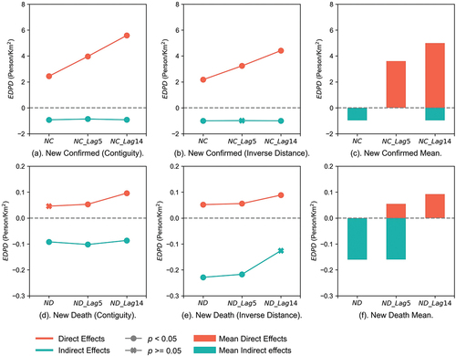
We determine that in the SDMs with the same dependent variables, for the results by using a contiguity and inverse distance matrixes, if both of them are significant (p < 0.05), then the impact of NPD on the dependent variables are significant. Otherwise, we state that there were no obvious effects of the NPD. Then, the mean effect values of the two spatial matrixes are computed. Thus, in Figure 4, according to (a) and (b), the mean and significant results are plotted in (c). While (d) and (c) determine the (f).

It is evident that in terms of the ND-SDM, the direct effect is not significant but significant indirect effects are plotted, while the other two NPD (i.e. EDPD) in Figure 4 (c) only have significant direct effects. In terms of the new death case-dependent variables, the coefficients in ND_Lag5-SDM have both significant direct and indirect effects, while the direct effects are positive but indirect effects are negative. However, the coefficient in ND_Lag14-SDM is only significantly positive for the direct effect, and ND is only significantly negative for the indirect effect.

4.6 Validation

This section illustrates the validation results using the two validation strategies.

4.6.1 VS1

$\mathit{R}{I}_{\mathit{coef}.}$ and $\mathit{R}{I}_{\mathit{sig}.}$ of the random experiment are shown in Table 5. In terms of the main results of SDE models, all RIs of the NPD coefficient are more than 60%, but the significance RIs can partly reach 100%, while others are much lower. The $\mathit{R}{I}_{\mathit{coef}.}$ of the direct effects for NPD are all more than 60% over the 12 SDE models as well, while the corresponding $\mathit{R}{I}_{\mathit{sig}.}$ has the same patterns as the main results. In terms of the indirect effects, except when the dependent variable is NC_Lag14, the $\mathit{R}{I}_{\mathit{coef}.}$ for others are all above 50%, while $\mathit{R}{I}_{\mathit{sig}.}$ for only three of them is less than 50%.

Table 5. $\mathit{R}{\mathit{I}}_{\mathit{coef}.}$ and $\mathit{R}{\mathit{I}}_{\mathit{sig}.}$ of VS1.

		Contiguity Matrix								Inverse Distance Matrix
	NC		NC_Lag5	NC_Lag14	ND	ND_Lag5	ND_Lag14		NC	NC_Lag5	NC_Lag14	ND	ND_Lag5	ND_Lag14
Main
$\mathit{R}{I}_{\mathit{coef}.}$	61.50%		61.68%	65.35%	94.16%	95.19%	83.82%		66.00%	64.30%	66.53%	97.60%	93.58%	88.31%
$\mathit{R}{I}_{\mathit{sig}.}$	40%		100%	100%	20%	20%	100%		20%	100%	100%	20%	20%	100%
Dir.
$\mathit{R}{I}_{\mathit{coef}.}$	62.59%		61.79%	65.06%	92.65%	94.02%	83.75%		65.53%	64.46%	67.39%	97.68%	93.81%	88.41%
$\mathit{R}{I}_{\mathit{sig}.}$	40%		100%	100%	20%	20%	100%		10%	100%	100%	20%	20%	100%
Ind.
$\mathit{R}{I}_{\mathit{coef}.}$	55.95%		60.06%	62.66%	58.35%	63.36%	73.86%		61.85%	62.29%	31.42%	83.63%	88.80%	66.96%
$\mathit{R}{I}_{\mathit{sig}.}$	100%		20%	100%	70%	100%	50%		80%	10%	90%	50%	50%	20%

Note: Dir. and Ind. refers to the direct and indirect effects.

The validation by using the random experiment strategy can compute the reliability of both coefficients and significance, which overall supports the main results based on all six dependent variables and the two spatial weights matrices.

Full regression results of the SDE models for the 10 random experiments are reported in Table A.5 to A.24 in Appendix 3.

4.6.2 VS2

Table 6 illustrates the results of the SDE model for VS2. The consistency comparison with the original results is shown as well, where the corresponding coefficients with significance are tabulated. The full regression results are shown in Table A.25 and A.26 in Appendix 4.

Table 6. SDE model results of VS2

	Contiguity Matrix				Inverse Distance Matrix
	NC	NC_Lag5	ND	ND_Lag5	NC	NC_Lag5	ND	ND_Lag5
Main	2.674***	1.689*	0.137***	0.102***	3.166***	2.114**	0.164***	0.121***
Cons.	+/+	+/+	+/+	+/+	+/+	+/+	+/+	+/+
Dir.	2.628***	1.659*	0.134***	0.0997***	3.123***	2.083**	0.161***	0.119***
Cons.	+/+	+/+	+/+	+/+	+/+	+/+	+/+	+/+
Ind.	−3.605*	−2.467	−0.183***	−0.139***	−30.84***	−23.22**	−1.687***	−1.201***
Cons.	+/+	+/-	+/+	+/+	+/+	+/-	+/+	+/+

Note: Dir. and Ind. refers to the direct and indirect effects. Cons. indicates the consistency. The left sign of the consistencies represents the consistency of positive/negative, while the right one represents the consistency of significance. “+” means they are consistent, while “-” means they are contrary. For example, “Cons.” under “Ind.” on the second column is “+/+”, which means the indirect effects coefficient of BMNI and NPD for NC_Lag5-SDE models are consistent (“+”), they are all positive, while the right one for the significance are inconsistent (“-”), the BMNI one is insignificant, while the NPD one is significant.

The consistency tuple of signs for each dependent variable based on two kinds of spatial weights matrices illustrates that only two tuples are inconsistent. While others, including the positive or negative of coefficients with their significance are all consistent, which means the results of VS2 are more than 95% consistent on a qualitative scale. These results validate our original qualitative results at a much high level of reliability and robustness.

5. Discussion

Overall, dynamic population density changes put a significant impact on the pandemic of COVID-19 based on the significant coefficients of NPD in all SDMs, which support similar opinions in other surveyed studies (Rader et al. 2020; Li et al. 2020; Kraemer et al. 2020). The most significant positive global Moran’s Is for monthly average-dependent variables show that the transmission of COVID-19 features spatial dependencies. Further, according to the results in Table 2, the spatial lag coefficients δ in all 12 SDMs are significantly positive. Thus, spatial features play a key role in the analysis of how dynamic population density can impact the transmission of COVID-19. This also shows that transmission of COVID-19 is impacted by the local dynamic population density changes, as well as the density changes in neighboring regions, and these relationships have a positive correlation.

In Table A.3 and A.4, the overall spatial lag coefficients δ using an inverse distance spatial matrix are higher than that using a contiguity matrix (the average coefficients are 0.292 and 0.122 respectively). This means the transmission varies as the spatial distance increase from the local region, and is not limited just to the adjacent regions. This result highlights that when detecting factors that impact the transmission of the COVID-19, we need to consider spatial regression models. However, because these two spatial matrices emphasize different significances, we explain the results, respectively.

When using a contiguity weights matrix, all the coefficients of NPD are significant except for ND-SDM (Table 4). This result illustrates that between two adjacent administrative units, there is an obvious effect of population density changes on the transmission of COVID-19, where we define this as the spatial contiguity effect. Dynamic population density changes directly and significantly influence the transmission of the virus. To be more specific, when NPD increases by 1 unit in quantity, the new confirmed case number of the day in a county grows by 0.101, while the number after 5 days grows by 0.131, and after 14 days increases by 0.154. This phenomenon relies on the mechanism of human-to-human contact. Meanwhile, under the condition that NPD increases the same unity quantity, the new confirmed case number increases with the time lags, which means the transmission of COVID-19 impacted by the dynamic population density changes is likely to take more than 14 days. However, when NPD increases by 1 unit in quantity in a county, the new confirmed cases in neighbor counties would decrease by 0.207, while the number after 5 days falls by 0.160, and after 14 days reduces by 0.205. There may be two reasons for these results. First, when the local new confirmed cases increase, governments would publish and strengthen strict intervention measurements to control the spread of cases and the virus, for example, to restrict road and foot travel using road blocks. These policies can reduce a neighbor (e.g. B county) being impacted by the confirmed cases (that have been found), while more potential cases that have not to be confirmed would spread to neighbor regions. This means local potential cases (not the locally confirmed cases) might increase the neighbor’s confirmed cases. Second, in terms of a neighbor B county, when more confirmed cases in A county are reported, the measures of B county would help protect the spread of the virus as well, which includes both the government’s control and the self-defense of citizens in B county (Zhu et al. 2021).

Similarly, the contiguity spatial effect of the impact of dynamic population density changes on the new death cases is intuitive as well. The insignificant coefficient of NPD in ND-SDM (0.00366, p ≥ 0.05) shows that the dynamic population density changes during a day would not result in death case of COIVD-19 rising on that day, because of the human immune system resistance and timely medical intervention measures. The infectee would not die in one day (the time between symptom onset and death ranged from about 2 weeks to 8 weeks (World Health Organization (WHO) 2020c)). However, 1 unit quantity increase of NPD can lead to 0.004,23 people dead after 5 days, and 0.007,49 deaths after 14 days, locally. But indirectly, the increase of people’s density can raise the probability of survival in neighbor regions, wherein neighbor B there are 0.007,87 people that survive from COVID-19 on a day when the NPD increases 1 unit quantity in local A, while after 5 days, 0.008,79 people survive in county B and after 14 days there are 0.007,39 fewer people dead. The reasons are similar to the explanation for the new confirmed case SDMs above.

When using an inverse distance weight matrix (Table 4), with the geographical distance reduces, the spatial effect of the dynamic population density changes impacts on the transmission of COVID-19 varies, and this effect is defined as the spatial attenuation effect. There are significant and insignificant coefficients of NPD (insignificant results are more than significant ones) when using the matrix, which means the spatial attenuation effect is weaker than a spatial contiguity effect in terms of the impact of people’s density on the transmission of COVID-19. To be more specific, when NPD increases 1 unit in quantity, the local new confirmed case number increases by 0.094,4, but after 5 days, the new confirmed case grows by 0.118, and increases by 0.138 after 14 days. Meanwhile, other regions that are not limited to the adjacency neighbor counties but are further away from nonadjacency counties, they decrease by 0.712 confirmed cases at the day and decrease by 0.566 after 14 days, but after 5 days the influence of dynamic population density changes is not clear. The reason is that a 5-day is too short a time slot to accurately register new COVID-19 infections. And as the spatial area is extended, the indirect spatial attenuation effect disappears as time goes on.

However, in terms of the spatial attenuation effect for the death case, when local NPD increases by 1 unit quantity in that first day, after 5 days and 14 days, the death case number increases by 0.004,13, 0.004,44, and 0.006,93, respectively. This means that when a direct spatial attenuation effect occurs, the change of people’s density impacts the local death case. But in terms of other regions, the indirect effects are only significant for ND-SDM (−0.0212, p < 0.01) and ND_Lag5-SDM (−0.02, p < 0.01). These results are further evidence that with the extension of the spatial impact the prolongation of the temporal impact, the influence of local dynamic population density changes on the transmission of COVID-19 in other regions, fades.

To compute the quantitative impact of the people’s density on the new confirmed and death cases of COVID-19 in China over the study period, we use Equation (18)(18) $ln\left(\mathit{ATPD}+1\right)=0.0817\times ln\left(\mathit{EPD}+1\right)$(18) , to transfer the NPD to a real people’s density (EDPD). At the same time, we calculate the mean values of the coefficients when using two different spatial matrixes to determine the overall quantitative impacts. Furthermore, the average $\mathit{R}{I}_{\mathit{coef}.}$ and $\mathit{R}{I}_{\mathit{sig}.}$ are also given, see below.

Figure 4(c), (f) give the detailed results. To be more specific, nationwide, on average, when the population density increases 1 Person/km² hourly in a county, after 5 days, the county would have 3.6 more new confirmed cases ($\mathit{R}{I}_{\mathit{coef}.}$ = 63.13%, $\mathit{R}{I}_{\mathit{sig}.}$ = 100%) and 0.054 new death cases ($\mathit{R}{I}_{\mathit{coef}.}$ = 93.92%, $\mathit{R}{I}_{\mathit{sig}.}$ = 20%), while after 14 days, there are 5 new confirmed cases ($\mathit{R}{I}_{\mathit{coef}.}$ = 66.25%, $\mathit{R}{I}_{\mathit{sig}.}$ = 100%) and 0.092 new death cases ($\mathit{R}{I}_{\mathit{coef}.}$ = 86.08%, $\mathit{R}{I}_{\mathit{sig}.}$ = 100%). But in terms of the neighboring regions, on the day and after 14 days, when population density changes, there are 0.960 ($\mathit{R}{I}_{\mathit{coef}.}$ = 58.9%, $\mathit{R}{I}_{\mathit{sig}.}$ = 90%) and 0.959 ($\mathit{R}{I}_{\mathit{coef}.}$ = 47.04%, $\mathit{R}{I}_{\mathit{sig}.}$ = 95%) fewer people to be confirmed to be infected by COVID-19, while 0.160 ($\mathit{R}{I}_{\mathit{coef}.}$ = 70.99%, $\mathit{R}{I}_{\mathit{sig}.}$ = 60%) and 0.159 ($\mathit{R}{I}_{\mathit{coef}.}$ = 76.08%, $\mathit{R}{I}_{\mathit{sig}.}$ = 75%) people survive on the day and after 5 days.

In terms of the influence of other supplementary dependent variables shown in Table 4, socioeconomic factors have not proved to have a significant impact on the transmission of COVID-19 in this study (for the reasons already given). For the environmental factors, NO₂ as a key pollutant of air pollution also plays a key role in the transmission of COVID-19. Because NO₂ is a diffusive gas whose concentration attenuates with distance (Massman 1998), a model using an inverse distance spatial matrix is more interpretable than using a contiguity matrix. Thus, according to the results of SDMs using an inverse distance matrix, the indirect effects of NO₂ concentration are significantly positive, but the indirect effects are significantly negative. This result is similar to the study of Ogen and Yaron (Ogen 2020), who explain that a high NO₂ concentration accompanied by a downwards airflow causes a NO₂ buildup close to the surface, which prevents the dispersion of air pollutants. This phenomenon can cause a high incidence of respiratory problems and inflammation in the local population, which contributes to the high COVID-19 fatality rates in these regions. Our study also provides evidence that NO₂ is likely to be one of the causes of higher local infections and even deaths due to COVID-19 (direct effect). Meanwhile, this kind of effect prevents the large-scale spread of NO₂, causing ab insignificant increase of NO₂ concentration around a county (indirect effect). This effect does not speed up the spread of the surrounding pandemic (the coefficients are negative).

In terms of other environmental factors including both air pollution and weather conditions, just like with NO₂, they all attenuate with increased distance. Thus, the results computed by using an inverse distance matrix are more interpretable. TP, DP, SO2, PM25, and PM10 all have a significant impact on the spread of the pandemic in certain SDMs. For example, five SDMs show that SO₂ has a significant positive indirect effect on the newly confirmed cases and on death cases. In addition, the significant results of TP, DP, SO2, PM25, and PM10 in certain models can also prove other relevant research results. However, this paper focuses on the impact of dynamic population density changes on the pandemic situation, so other supplementary variables are not discussed in depth here.

6. Conclusion

Dynamic population density changes which lead to the change of people’s density has a significant impact on the transmission of COVID-19, where the impact is spatiotemporal related and estimated quantitatively. To be more specific, dynamic population density changes in one county not only impact the daily new confirmed and death cases of the local county but also influence the transmission of COVID-19 in the neighboring counties. Further, dynamic population density changes on the day not only impacts the transmission of the virus on that day but also influence the situations in the future (e.g. 5 and 14 day lags). This study not only provides estimated quantitative values, but the reliability of these numbers is also quantified.

For the case that a pandemic, such as COVID-19 is still ongoing, even if more and more people are vaccinated, a new mutant strain may need to restart the same measures to try to contain the new pandemic strain in human society via restricting human mobility en masse in a measured way. Therefore, for such a pandemic laden world, this paper proposes some additional clear policy implications: from a public health perspective, for policymakers and governments all over the world that not only should citizens aim to maintain a social distance between individuals of a specific length, e.g. 2 m but that we also consider certain place restrictions on crowd activities with quantitative restrictions. These restrictions can cover a large region like a county or can include a smaller area, such as an indoor space, for example, limiting the number or density of people in shopping malls which can be computed by the historical dynamic population density data, to reduce the diagnosis rate and mortality rate on that day and in the future. Moreover, when any county-level government authority considers instigating COVID-19 related mobility policy restrictions, good cooperation with adjacent counties that can maximize the best interests of the population as a whole is needed, because both local and neighboring counties’ dynamic population density changes can impact the transmission of the virus, and these direct and indirect effects may be quite different. Furthermore, from the perspective of resource exploitation, access to open (spatial) data, such as volunteered GIS data, plays a more and more vital role than before, especially for the COVID-19 pandemic. Traditional governments need to set up a special policy research department to make available and exploit such datasets using state-of-the-art technology to be able to make more efficient policies that relate to such spatial and temporal quantitative measurements.

There are some limitations of this study that could be future work. First, the spatial and temporal resolutions of the dataset only reach the county level (in space) and hour level (in time). For more accurate pandemic prevention measures, higher spatial and temporal resolutions are still needed, such as population density changes at a kilometer and minute levels. Second, under the premise of a certain range of vaccination, the transmission mechanism of the pandemic situation may be significantly different from that of a non-vaccinated region. Therefore, projects that focus on vaccination should not only consider the temporal aspect; the spatial model needs to be improved too. Finally, different countries or regions have different pandemic environments, demographics, geographical topologies, transport links, and government measures. The quantitative results in this paper are not applicable equally to all regions or countries. Therefore, future research is needed to better understand the effect of such different national conditions and spatial-temporal population density changes in relation to pandemic situations.

Author contributions

Guangyuan Zhang: Experiment design and data curation, formal analysis, writing original draft; Stefan Poslad: Conceptualization, supervision, writing, reviews and editing; Yonglei Fan: Investigation, visualisation, software resources; Xiaoping Rui: Methodology, supervision, project administration.

Data Availability Statement

The authors confirm that the data and the code supporting the findings of this study are available within the article and its supplementary materials.

Disclosure statement

No potential conflict of interest was reported by the author(s).

Supplementary material

Supplemental data for this article can be accessed online at https://doi.org/10.1080/10095020.2022.2066576

Additional information

Funding

This research received funding from the National Science and Technology Major Project of the Ministry of Science and Technology of China [grant number 2017YFB0503605], the National Natural Science Foundation of China [grant number 41771478], the Fundamental Research Funds for the Central Universities [grant number 2019B02514], Natural Science Foundation of Beijing, China [grant number 8172046], the China Scholarship Council (CSC), and Queen Mary University of London.

Notes on contributors

Guangyuan Zhang

Guangyuan Zhang received BSc and MSc in Geographical Information Science, from Hefei University of Technology, and University of Chinese Academy of Sciences, China. He received the PhD degree in Computer Science from Queen Mary University of London, UK. His research interest includes Internet of Behaviors and Urban Computing.

Stefan Poslad

Stefan Poslad received the PhD from Newcastle University. He is currently an Associate Professor at Queen Mary University of London, UK, where he heads the IoT Lab. His research interests are Internet of Things, ubiquitous computing, semantic Web, and distributed system management.

Yonglei Fan

Yonglei Fan received BSc and MSc from South China Normal University and University of Chinese Academy of Sciences, China. He is currently pursuing a PhD degree in Computer Science at Queen Mary University of London, UK. His research interests are Geographical Information Science, indoor poisoning technique, human activity recognition and Internet of Things.

Xiaoping Rui

Xiaoping Rui received PhD degree in Cartography and Geographic Information System from the Graduate University of Chinese Academy of Sciences, Beijing, China, in 2004. He is currently a full professor with the School of Earth Sciences and Engineering, Hohai University. His research interests include geographical big data mining, 3D visualization of spatial data, and remote sensing image understanding.

References

- Alexander, N., A. Lenhart, K. Anaya-Izquierdo, and M.S. Carvalho. 2020. “Spatial Spillover Analysis of a Cluster-randomized Trial against Dengue Vectors in Trujillo, Venezuela.” PLoS Neglected Tropical Diseases 14 (9): e0008576. doi:10.1371/journal.pntd.0008576.
- Alin, A. 2010. “Multicollinearity.” Wiley Interdisciplinary Reviews. Computational Statistics 2 (3): 370–374. doi:10.1002/wics.84.
- Andersen, L.M., S.R. Harden, M.M. Sugg, J.D. Runkle, and T.E. Lundquist. 2021. “Analyzing the Spatial Determinants of Local Covid-19 Transmission in the United States.” Science of the Total Environment 754: 142396. doi:10.1016/j.scitotenv.2020.142396.
- Anselin, L., and D.A. Griffith. 1988. “Do Spatial Effects Really Matter in Regression Analysis?” Papers in Regional Science 65 (1): 11–34. doi:10.1111/j.1435-5597.1988.tb01155.x.
- Arif, M., and S. Sengupta. 2021. “Nexus between Population Density and Novel Coronavirus (COVID-19) Pandemic in the South Indian States: A Geo-statistical Approach.” Environment, Development and Sustainability 23 (7): 10246–10274. doi:10.1007/s10668-020-01055-8.
- Backer, J.A., D. Klinkenberg, and J. Wallinga. 2020. “Incubation Period of 2019 Novel Coronavirus (2019-ncov) Infections among Travellers from Wuhan, China, 20–28 January 2020.” Eurosurveillance 25 (5): 2000062. doi:10.2807/1560-7917.ES.2020.25.5.2000062.
- Bag, R., M. Ghosh, B. Biswas, and M. Chatterjee. 2020. “Understanding the Spatio‐temporal Pattern of COVID‐19 Outbreak in India Using GIS and India’s Response in Managing the Pandemic.” Regional Science Policy & Practice 12 (6): 1063–1103. doi:10.1111/rsp3.12359.
- Baidu Migration Data (accessed 1 June 2021). https://qianxi.baidu.com/.
- Bao, J., H. Lin, and Q. Zhou. 2020. “COVID-19 Epidemic Spatio-Temporal Dataset User Guide.” Accessed Feb 18. https://github.com/Estelle0217/COVID-19-Epidemic-Dataset.git .
- Bashir, M.F., B. Ma, M. A. Bashir, M.A. Bashir, M. Bashir, M. Bashir, and M. Bashir. 2020. “Correlation between Climate Indicators and COVID-19 Pandemic in New York, USA.” Science of the Total Environment 728: 138835. doi:10.1016/j.scitotenv.2020.138835.
- Baum, C.F., and M. Henry. 2020. “Socioeconomic Factors Influencing the Spatial Spread of COVID-19 in the United States.” Miguel, Socioeconomic Factors Influencing the Spatial Spread of COVID-19 in the United States (May 29, 2020). doi:10.2139/ssrn.3614877.
- Becker, S., and J.M. Soukup. 1999. “Exposure to Urban Air Particulates Alters the Macrophage-mediated Inflammatory Response to Respiratory Viral Infection.” Journal of Toxicology and Environmental Health. Part A 57 (7): 445–457. doi:10.1080/009841099157539.
- Berk, R.A. 1983. “An Introduction to Sample Selection Bias in Sociological Data.” American Sociological Review 48 (3): 386–398. doi:10.2307/2095230.
- Cai, Q., J. Lu, Q. Xu, Q. Guo, X. De, Q. Sun, H. Yang, G. Zhao, and Q. Jiang. 2007. “Influence of Meteorological Factors and Air Pollution on the Outbreak of Severe Acute Respiratory Syndrome.” Public Health 121 (4): 258–265. doi:10.1016/j.puhe.2006.09.023.
- Centers for Disease Control and Prevention (CDC). 2020. “Interactive Atlas of Heart Disease and Stroke.” https://nccd.cdc.gov/DHDSPAtlas/Reports.aspx .
- CEPI. 2021. ”CEPI Survey Assesses Potential COVID-19 Vaccine Manufacturing Capacity.” Accessed 1 June 2021.https://cepi.net/news_cepi/cepi-survey-assesses-potential-covid-19-vaccine-manufacturing-capacity/ .
- Chen, Y., F. Li, J. Chen, B. Du, -K.-K.R. Choo, and H. Hassan. 2017. “EPLS: A Novel Feature Extraction Method for Migration Data Clustering.” Journal of Parallel and Distributed Computing 103: 96–103. doi:10.1016/j.jpdc.2016.11.008.
- Chen, B., H. Liang, X. Yuan, Y. Hu, M. Xu, Y. Zhao, B. Zhang, F. Tian, and X. Zhu. 2020a. “Roles of Meteorological Conditions in COVID-19 Transmission on a Worldwide Scale.” medRxiv. doi:10.1101/2020.03.16.20037168.
- Chen, Z., Q. Zhang, Y. Lu, Z. Guo, X. Zhang, W. Zhang, C. Guo, C. Liao, Q. Li, and X. Han. 2020b. “Distribution of the COVID-19 Epidemic and Correlation with Population Emigration from Wuhan, China.” Chinese Medical Journal 133 (9): 1044–1050. doi:10.1097/CM9.0000000000000782.
- Elhorst, J.P. 2001. “Dynamic Models in Space and Time.” Geographical Analysis 33 (2): 119–140. doi:10.1111/j.1538-4632.2001.tb00440.x.
- Elhorst, J.P. 2014. Spatial Econometrics: From Cross-sectional Data to Spatial Panels. Vol. 479. Heidelberg: Springer.
- ESRI. “What Is a Shapefile?”. https://desktop.arcgis.com/en/arcmap/10.3/manage-data/shapefiles/what-is-a-shapefile.htm. Accessed 1 June 2021.
- European Centre for Disease Prevention and Control (ECDC). 2021. “COVID-19 Situation Update Worldwide.” https://www.ecdc.europa.eu/en/geographical-distribution-2019-ncov-cases. Accessed 1 June 2021.
- Fouillet, A., I. Pontais, and C. Caserio-Schönemann. 2020. “Excess All-cause Mortality during the First Wave of the COVID-19 Epidemic in France, March to May 2020.” Eurosurveillance 25 (34): 2001485. doi:10.2807/1560-7917.ES.2020.25.34.2001485.
- Ge, M., and Z. Feng. 2010. “Classification of Densities and Characteristics of Curve of Population Centers in China by GIS.” Journal of Geographical Sciences 20 (4): 628–640. doi:10.1007/s11442-010-0628-5.
- Goodchild, M.F. 1986. Spatial Autocorrelation. Vol. 47. Norwich, England, UK: Geo Books.
- Griffith, D.A. 1988. “Estimating Spatial Autoregressive Model Parameters with Commercial Statistical Packages.” Geographical Analysis 20 (2): 176–186. doi:10.1111/j.1538-4632.1988.tb00174.x.
- Griffith, D., and B. Li. 2021. “Spatial-temporal Modeling of Initial COVID-19 Diffusion: The Cases of the Chinese Mainland and Conterminous United States.” Geo-spatial Information Science 24 (3): 340–362. doi:10.1080/10095020.2021.1937338.
- Gross, B., Z. Zheng, S. Liu, X. Chen, A. Sela, J. Li, D. Li, and S. Havlin. 2020. “Spatio-temporal Propagation of COVID-19 Pandemics.” EPL (Europhysics Letters) 131 (5): 58003. doi:10.1209/0295-5075/131/58003.
- Guan, W., Z. Ni, Y. Hu, W. Liang, C. Ou, J. He, L. Liu, H. Shan, C. Lei, and D.S. Hui. 2020. “Clinical Characteristics of Coronavirus Disease 2019 in China.” New England Journal of Medicine 382 (18): 1708–1720. doi:10.1056/NEJMoa2002032.
- Guliyev, H. 2020. “Determining the Spatial Effects of COVID-19 Using the Spatial Panel Data Model.” Spatial Statistics 38: 100443. doi:10.1016/j.spasta.2020.100443.
- Hadjidemetriou, G.M., M. Sasidharan, G. Kouyialis, and A.K. Parlikad. 2020. “The Impact of Government Measures and Human Mobility Trend on COVID-19 Related Deaths in the UK.” Transportation Research Interdisciplinary Perspectives 6: 100167. doi:10.1016/j.trip.2020.100167.
- Hausman, J.A. 1978. “Specification Tests in Econometrics.” Econometrica: Journal of the Econometric Society 46 (6): 1251–1271. doi:10.2307/1913827.
- Horne, B.D., E.A. Joy, M.G. Hofmann, P.H. Gesteland, J.B. Cannon, J.S. Lefler, D.P. Blagev, E.K. Korgenski, N. Torosyan, and G.I. Hansen. 2018. “Short-term Elevation of Fine Particulate Matter Air Pollution and Acute Lower Respiratory Infection.” American Journal of Respiratory and Critical Care Medicine 198 (6): 759–766. doi:10.1164/rccm.201709-1883OC.
- Hsiao, C. 2005. “Why Panel Data?” The Singapore Economic Review 50 (2): 143–154. doi:10.1142/S0217590805001937.
- Hu, M., J.D. Roberts, G.P. Azevedo, and D. Milner. 2021. “The Role of Built and Social Environmental Factors in Covid-19 Transmission: A Look at America’s Capital City.” Sustainable Cities and Society 65: 102580. doi:10.1016/j.scs.2020.102580.
- Huang, J., H. Wang, M. Fan, A. Zhuo, Y. Sun, and Y. Li. 2020b. “Understanding the Impact of the COVID-19 Pandemic on Transportation-related Behaviors with Human Mobility Data.” Paper presented at the Proceedings of the 26th ACM SIGKDD International Conference on Knowledge Discovery & Data Mining. New York, United States, July 6-10.
- Huang, H., Y. Wang, Z. Wang, Z. Liang, S. Qu, S. Ma, G. Mao, and X. Liu. 2020a. “Epidemic Features and Control of 2019 Novel Coronavirus Pneumonia in Wenzhou, China.” China (3/3/2020). doi:10.2139/ssrn.3550007.
- James, G., D. Witten, T. Hastie, and R. Tibshirani. 2013. An Introduction to Statistical Learning. Vol. 112. New York: Springer.
- Jiang, P., X. Fu, Y. Van Fan, J.J. Klemeš, P. Chen, S. Ma, and W. Zhang. 2021. “Spatial-temporal Potential Exposure Risk Analytics and Urban Sustainability Impacts Related to COVID-19 Mitigation: A Perspective from Car Mobility Behaviour.” Journal of Cleaner Production 279: 123673. doi:10.1016/j.jclepro.2020.123673.
- Jiang, B., and C.D. Rijke. 2021. “A Power-law-based Approach to Mapping COVID-19 Cases in the United States.” Geo-spatial Information Science 24 (3): 333–339. doi:10.1080/10095020.2020.1871306.
- Kang, D., H. Choi, J.-H. Kim, and J. Choi. 2020. “Spatial Epidemic Dynamics of the COVID-19 Outbreak in China.” International Journal of Infectious Diseases 94: 96–102. doi:10.1016/j.ijid.2020.03.076.
- Kim, J.H., F. Marks, and J.D. Clemens. 2021. “Looking beyond COVID-19 Vaccine Phase 3 Trials.” Nature Medicine 27 (2): 205–211. doi:10.1038/s41591-021-01230-y.
- Kontis, V., J.E. Bennett, T. Rashid, R.M. Parks, J. Pearson-Stuttard, M. Guillot, P. Asaria, B. Zhou, M. Battaglini, and G. Corsetti. 2020. “Magnitude, Demographics and Dynamics of the Effect of the First Wave of the COVID-19 Pandemic on All-cause Mortality in 21 Industrialized Countries.” Nature Medicine 26 (12): 1919–1928. doi:10.1038/s41591-020-1112-0.
- Kraemer, M.U., T.A. Perkins, D.A. Cummings, R. Zakar, S.I. Hay, D.L. Smith, and R. Reiner Jr. 2015. “Big City, Small World: Density, Contact Rates, and Transmission of Dengue across Pakistan.” Journal of the Royal Society Interface 12 (111): 20150468. doi:10.1098/rsif.2015.0468.
- Kraemer, M.U., C.-H. Yang, B. Gutierrez, C.-H. Wu, B. Klein, D.M. Pigott, L. Du Plessis, N.R. Faria, R. Li, and W.P. Hanage. 2020. “The Effect of Human Mobility and Control Measures on the COVID-19 Epidemic in China.” Science 368 (6490): 493–497. doi:10.1126/science.abb4218.
- Lai, S., E. Erbach-Schoenberg, C. Pezzulo, N.W. Ruktanonchai, A. Sorichetta, J. Steele, T. Li, C.A. Dooley, and A.J. Tatem. 2019. “Exploring the Use of Mobile Phone Data for National Migration Statistics.” Palgrave Communications 5 (1): 1–10. doi:10.1057/s41599-019-0242-9.
- LeSage, J.P., and R.K. Pace. 2008. “Spatial Econometric Modeling of Origin‐destination Flows.” Journal of Regional Science 48 (5): 941–967. doi:10.1111/j.1467-9787.2008.00573.x.
- LeSage, J.P., and R.K. Pace. 2009. Introduction to Spatial Econometrics. New York, USA: Chapman and Hall/CRC.
- Li, H., C.A. Calder, and N. Cressie. 2007. “Beyond Moran’s I: Testing for Spatial Dependence Based on the Spatial Autoregressive Model.” Geographical Analysis 39 (4): 357–375. doi:10.1111/j.1538-4632.2007.00708.x.
- Li, Q., X. Guan, P. Wu, X. Wang, L. Zhou, Y. Tong, R. Ren, K.S. Leung, E.H. Lau, and J.Y. Wong. 2020. “Early Transmission Dynamics in Wuhan, China, of Novel Coronavirus–infected Pneumonia.” New England Journal of Medicine 382 (13): 1199–1207. doi:10.1056/NEJMoa2001316.
- Li, B., and L. Ma. 2020. “Migration, Transportation Infrastructure, and the Spatial Transmission of COVID-19 in China.” Journal of Urban Economics 15: 103351.
- Liu, J., J. Zhou, J. Yao, X. Zhang, L. Li, X. Xu, X. He, B. Wang, S. Fu, and T. Niu. 2020. “Impact of Meteorological Factors on the COVID-19 Transmission: A Multi-city Study in China.” Science of the Total Environment 726: 138513. doi:10.1016/j.scitotenv.2020.138513.
- Ma, Y., Y. Zhao, J. Liu, X. He, B. Wang, S. Fu, J. Yan, J. Niu, J. Zhou, and B. Luo. 2020. “Effects of Temperature Variation and Humidity on the Death of COVID-19 in Wuhan, China.” Science of the Total Environment 724: 138226. doi:10.1016/j.scitotenv.2020.138226.
- Massman, W. 1998. “A Review of the Molecular Diffusivities of H2O, CO2, CH4, CO, O3, SO2, NH3, N2O, NO, and NO2 in Air, O2 and N2 near STP.” Atmospheric Environment 32 (6): 1111–1127. doi:10.1016/S1352-2310(97)00391-9.
- Meade, M.S. 2014. “Medical Geography.” The Wiley Blackwell Encyclopedia of Health, Illness, Behavior, and Society 1375–1381. doi:10.1002/9781118410868.wbehibs204.
- Mollalo, A., B. Vahedi, and K.M. Rivera. 2020. “GIS-based Spatial Modeling of COVID-19 Incidence Rate in the Continental United States.” Science of the Total Environment 728: 138884. doi:10.1016/j.scitotenv.2020.138884.
- Murano, Y., R. Ueno, S. Shi, T. Kawashima, Y. Tanoue, S. Tanaka, S. Nomura, H. Shoji, T. Shimizu, and H. Nguyen. 2021. “Impact of Domestic Travel Restrictions on Transmission of COVID-19 Infection Using Public Transportation Network Approach.” Scientific Reports 11 (1): 1–9. doi:10.1038/s41598-021-81806-3.
- National Health Commission of the People’s Republic of China. “China Health Statistics Yearbook 2020 .” http://www.nhc.gov.cn/zwgk/tjnj1/ejlist.shtml. Accessed 1 June 2021.
- National Urban Air Quality Real Time Release Platform http://www.cnemc.cn/sssj/ . Accessed 1 June 2021.
- Nishiura, H., N.M. Linton, and A.R. Akhmetzhanov. 2020. “Serial Interval of Novel Coronavirus (COVID-19) Infections.” International Journal of Infectious Diseases 93: 284–286. doi:10.1016/j.ijid.2020.02.060.
- NOAA National Centers for Environmental Information https://www.ncdc.noaa.gov/ . Accessed 1 June 2021.
- Ogen, Y. 2020. “Assessing Nitrogen Dioxide (NO2) Levels as a Contributing Factor to Coronavirus (COVID-19) Fatality.” Science of the Total Environment 726: 138605. doi:10.1016/j.scitotenv.2020.138605.
- Parker, E.P., M. Shrotri, and B. Kampmann. 2020. “Keeping Track of the SARS-CoV-2 Vaccine Pipeline.” Nature Reviews. Immunology 20 (11): 650. doi:10.1038/s41577-020-00455-1.
- Poole, L. 2020. “Seasonal Influences on the Spread of SARS-CoV-2 (COVID19), Causality, and Forecastabililty (3-15-2020).” Causality, and Forecastabililty (3-15-2020)(March 15, 2020). doi:10.2139/ssrn.3554746.
- Qi, H., S. Xiao, R. Shi, M.P. Ward, Y. Chen, W. Tu, Q. Su, W. Wang, X. Wang, and Z. Zhang. 2020. “COVID-19 Transmission in Mainland China Is Associated with Temperature and Humidity: A Time-series Analysis.” Science of the Total Environment 728: 138778. doi:10.1016/j.scitotenv.2020.138778.
- Rader, B., S.V. Scarpino, A. Nande, A.L. Hill, B. Adlam, R.C. Reiner, D.M. Pigott, B. Gutierrez, A.E. Zarebski, and M. Shrestha. 2020. “Crowding and the Shape of COVID-19 Epidemics.” Nature Medicine 26 (12): 1829–1834. doi:10.1038/s41591-020-1104-0.
- Rocklöv, J., and H. Sjödin. 2020. “High Population Densities Catalyse the Spread of COVID-19.” Journal of Travel Medicine 27 (3): taaa038. doi:10.1093/jtm/taaa038.
- Saffary, T., O.A. Adegboye, E. Gayawan, F. Elfaki, M.A. Kuddus, and R. Saffary. 2020. “Analysis of COVID-19 Cases’ Spatial Dependence in US Counties Reveals Health Inequalities.” Frontiers in Public Health 728. doi:10.3389/fpubh.2020.579190.
- Sajadi, M.M., P. Habibzadeh, A. Vintzileos, S. Shokouhi, F. Miralles-Wilhelm, and A. Amoroso. 2020. “Temperature, Humidity, and Latitude Analysis to Estimate Potential Spread and Seasonality of Coronavirus Disease 2019 (COVID-19).” JAMA network open 3 (6): e2011834–e. doi:10.1001/jamanetworkopen.2020.11834.
- Sannigrahi, S., F. Pilla, B. Basu, A.S. Basu, and A. Molter. 2020. “Examining the Association between Socio-demographic Composition and COVID-19 Fatalities in the European Region Using Spatial Regression Approach.” Sustainable Cities and Society 62: 102418. doi:10.1016/j.scs.2020.102418.
- Shariati, M., T. Mesgari, M. Kasraee, and M. Jahangiri-Rad. 2020. “Spatiotemporal Analysis and Hotspots Detection of COVID-19 Using Geographic Information System (March and April, 2020).” Journal of Environmental Health Science and Engineering 18 (2): 1499–1507. doi:10.1007/s40201-020-00565-x.
- Sugg, M.M., T.J. Spaulding, S.J. Lane, J.D. Runkle, S.R. Harden, A. Hege, and L.S. Iyer. 2020. “Mapping Community-level Determinants of COVID-19 Transmission in Nursing Homes: A Multi-scale Approach.” Science of the Total Environment 752: 141946. doi:10.1016/j.scitotenv.2020.141946.
- Sun, Y., X. Hu, and J. Xie. 2021. “Spatial Inequalities of COVID-19 Mortality Rate in Relation to Socioeconomic and Environmental Factors across England.” Science of the Total Environment 758: 143595. doi:10.1016/j.scitotenv.2020.143595.
- Tang, W., H. Liao, G. Marley, Z. Wang, W. Cheng, D. Wu, and R. Yu. 2020. “The Changing Patterns of Coronavirus Disease 2019 (COVID-19) in China: A Tempo geographic Analysis of the Severe Acute Respiratory Syndrome Coronavirus 2 Epidemic.” Clinical Infectious Diseases 71 (15): 818–824. doi:10.1093/cid/ciaa423.
- Tencent “Tencent Positioning Big Data.” https://heat.qq.com/ . Accessed 1 June 2021.
- Tian, H., Y. Liu, Y. Li, C.-H. Wu, B. Chen, M.U. Kraemer, B. Li, J. Cai, B. Xu, and Q. Yang. 2020. “An Investigation of Transmission Control Measures during the First 50 Days of the COVID-19 Epidemic in China.” Science 368 (6491): 638–642. doi:10.1126/science.abb6105.
- Van Doremalen, N., T. Bushmaker, D.H. Morris, M.G. Holbrook, A. Gamble, B.N. Williamson, A. Tamin, J.L. Harcourt, N.J. Thornburg, and S.I. Gerber. 2020. “Aerosol and Surface Stability of SARS-CoV-2 as Compared with SARS-CoV-1.” New England Journal of Medicine 382 (16): 1564–1567. doi:10.1056/NEJMc2004973.
- van Oosterhout, C., N. Hall, H. Ly, and K.M. Tyler. 2021. “COVID-19 Evolution during the pandemic–Implications of New SARS-CoV-2 Variants on Disease Control and Public Health Policies.” Virulence 12 (1): 507–508. doi:10.1080/21505594.2021.1877066.
- Verhagen, M.D., D.M. Brazel, J.B. Dowd, I. Kashnitsky, and M.C. Mills. 2020. “Forecasting Spatial, Socioeconomic and Demographic Variation in COVID-19 Health Care Demand in England and Wales.” BMC Medicine 18 (1): 1–11. doi:10.1186/s12916-020-01646-2.
- Wang, J., K. Tang, K. Feng, and W. Lv. 2020. “High Temperature and High Humidity Reduce the Transmission of COVID-19.” Available at SSRN 3551767. https://www.scienceopen.com/document_file/ff8b579c-26ff-4c3c-9aa5-a141bc8e35f6/PubMedCentral/ff8b579c-26ff-4c3c-9aa5-a141bc8e35f6.pdf .
- Wei, J., Y. Liu, Y. Zhu, J. Qian, R. Ye, C. Li, X. Ji, H. Li, C. Qi, and Y. Wang. 2020. “Impacts of Transportation and Meteorological Factors on the Transmission of COVID-19.” International Journal of Hygiene and Environmental Health 230: 113610. doi:10.1016/j.ijheh.2020.113610.
- Wei, S., and L. Wang. 2020. “Examining the Population Flow Network in China and Its Implications for Epidemic Control Based on Baidu Migration Data.” Humanities and Social Sciences Communications 7 (1): 1–10. doi:10.1057/s41599-020-00633-5.
- Wesolowski, A., N. Eagle, A.J. Tatem, D.L. Smith, A.M. Noor, R.W. Snow, and C.O. Buckee. 2012. “Quantifying the Impact of Human Mobility on Malaria.” Science 338 (6104): 267–270. doi:10.1126/science.1223467.
- Wooldridge, J.M. 2009. “Econometrics: Panel Data Methods.” https://www.cemmap.ac.uk/wp-content/legacy/uploads/cemmap/programmes/Background%20reading%20May%202016.pdf. Accessed 1 June 2021.
- World Economic Forum (WEF). 2021. “How China Pays for Its COVID-19 Medical Bills.” https://www.weforum.org/agenda/2020/12/how-china-pays-for-its-covid-19-medical-bills/. Accessed 1 June 2021.
- World Health Organization (WHO). 2020a. “Transmission of SARS-CoV-2: Implications for Infection Prevention Precautions.” https://apps.who.int/iris/bitstream/handle/10665/333114/WHO-2019-nCoV-Sci_Brief-Transmission_modes-2020.3-rus.pdf. Accessed 1 June 2021.
- World Health Organization (WHO). 2020b. “World Health Organization Coronavirus Disease (COVID-19) Dashboard.” https://covid19.who.int/. Accessed 1 June 2021.
- World Health Organization (WHO). 2020c. “Report of the WHO-China Joint Mission on Coronavirus Disease 2019 (COVID-19).” https://www.who.int/docs/default-source/coronaviruse/who-china-joint-mission-on-covid-19-final-report.pdf. Accessed 1 June 2021.
- Wu, X., R.C. Nethery, B.M. Sabath, D. Braun, and F. Dominici. 2020. “Exposure to Air Pollution and COVID-19 Mortality in the United States.” medRxiv. doi:10.1101/2020.04.05.20054502.
- Xie, Z., Y. Qin, Y. Li, W. Shen, Z. Zheng, and S. Liu. 2020. “Spatial and Temporal Differentiation of COVID-19 Epidemic Spread in Mainland China and Its Influencing Factors.” Science of the Total Environment 744: 140929. doi:10.1016/j.scitotenv.2020.140929.
- Xie, J., J. Teng, Y. Fan, R. Xie, and A. Shen. 2019. “The Short-term Effects of Air Pollutants on Hospitalizations for Respiratory Disease in Hefei, China.” International Journal of Biometeorology 63 (3): 315–326. doi:10.1007/s00484-018-01665-y.
- XINHUANET. 2021. “Backgrounder: Nationwide Aid to Hubei’s Battle against Coronavirus.” http://www.xinhuanet.com/english/2020-03/17/c_138888353.htm. Accessed 1 June 2021.
- Xiong, Y., Y. Wang, F. Chen, and M. Zhu. 2020. “Spatial Statistics and Influencing Factors of the Novel Coronavirus Pneumonia 2019 Epidemic in Hubei Province, China.” Research Square. doi:10.21203/rs.3.rs-16858/v1.
- Xu, X. 2017. ““China Population Spatial Distribution Kilometer Grid Dataset.” [In Chinese.] Data Registration and Publishing System of Data Center of Resources and Environment Science.” Chinese Academy of Sciences. doi:10.1207/82017121101.
- Xu, H., A. Berres, G. Thakur, J. Sanyal, and S. Chinthavali. 2021. “EPIsembleVis: A Geo-Visual Analysis and Comparison of the Prediction Ensembles of Multiple COVID-19 Models.” Journal of Biomedical Informatics 124: 103941. doi:10.1016/j.jbi.2021.103941.
- Xu, G., W. Wang, D. Lu, B. Lu, K. Qin, and L. Jiao. 2021. “Geographically Varying Relationships Between Population Flows from Wuhan and COVID-19 Cases in Chinese Cities.” Geo-Spatial Information Science 1–11. doi:10.1080/10095020.2021.1977093.
- Zhan, C., C.K. Tse, Y. Fu, Z. Lai, H. Zhang, and S.A. Cheong. 2020. “Modeling and Prediction of the 2019 Coronavirus Disease Spreading in China Incorporating Human Migration Data.” Plos one 15 (10): e0241171. doi:10.1371/journal.pone.0241171.
- Zhang, G., H. Lu, J. Dong, S. Poslad, R. Li, X. Zhang, and X. Rui. 2020a. “A Framework to Predict High-resolution Spatiotemporal PM2. 5 Distributions Using A Deep-learning Model: A Case Study of Shijiazhuang, China.” Remote Sensing 12 (17): 2825. doi:10.3390/rs12172825.
- Zhang, G., S. Poslad, X. Rui, G. Yu, Y. Fan, X. Song, and R. Li. 2021. “Using an Internet of Behaviours to Study How Air Pollution Can Affect People’s Activities of Daily Living: A Case Study of Beijing, China.” Sensors 21 (16): 5569. doi:10.3390/s21165569.
- Zhang, X., H. Rao, Y. Wu, Y. Huang, and H. Dai. 2020c. “Comparison of Spatiotemporal Characteristics of the COVID-19 and SARS Outbreaks in Mainland China.” BMC Infectious Diseases 20 (1): 1–7. doi:10.1186/s12879-020-05537-y.
- Zhang, G., X. Rui, and Y. Fan. 2018. “Critical Review of Methods to Estimate PM2. 5 Concentrations within Specified Research Region.” ISPRS International Journal of Geo-Information 7 (9): 368. doi:10.3390/ijgi7090368.
- Zhang, G., X. Rui, S. Poslad, X. Song, Y. Fan, and B. Wu. 2020b. “A Method for the Estimation of Finely-grained Temporal Spatial Human Population Density Distributions Based on Cell Phone Call Detail Records.” Remote Sensing 12 (16): 2572. doi:10.3390/rs12162572.
- Zheng, Z., and G. Zhang. 2020. “The Prediction of Finely-Grained Spatiotemporal Relative Human Population Density Distributions in China.” IEEE Access 8: 181534–181546. doi:10.1109/ACCESS.2020.3027824.
- Zhou, C., F. Su, T. Pei, A. Zhang, Y. Du, B. Luo, Z. Cao, J. Wang, W. Yuan, and Y. Zhu. 2020. “COVID-19: Challenges to GIS with Big Data.” Geography and Sustainability 1 (1): 77–87. doi:10.1016/j.geosus.2020.03.005.
- Zhu, Y., J. Xie, F. Huang, and L. Cao. 2020. “Association between Short-term Exposure to Air Pollution and COVID-19 Infection: Evidence from China.” Science of the Total Environment 727: 138704. doi:10.1016/j.scitotenv.2020.138704.
- Zhu, Y., S. Zhao, B. Qu, and R.J. Soares Magalhaes. 2021. “China’s COVID-19 Response for the Protection of Rural Communities.” PLoS Neglected Tropical Diseases 15 (2): e0009018. doi:10.1371/journal.pntd.0009018.