A novel unsupervised deep learning method for the generalization of urban form

ABSTRACT

Accurate delineation of urban form is essential to understand the impacts that urbanization has on the environment and regional climate. Conventional supervised classification of urban form requires a rigidly defined scheme and high-quality sample data with class labels. Due to the complexity of urban systems, it is challenging to consistently define urban form types and collect metadata to describe them. Therefore, in this study, we propose a novel unsupervised deep learning method for urban form delineation while avoiding the limitations of conventional supervised urban form classification methods. The novelty of the proposed method is the Multiscale Residual Convolutional Autoencoder (MRCAE), which can learn the latent representation of different urban form types. These vectors can be further used to generalize urban form types by using Self-Organizing Map (SOM) and the Gaussian Mixture Model (GMM). The proposed method is applied in the metropolitan area of Guangzhou-Foshan, China. The MRCAE model along with SOM and GMM is used to generalize the urban form types from satellite images. The physical and functional properties of each urban form type are also analyzed using several auxiliary datasets, including building footprints, Points-of-Interests (POIs) and Tencent User Density (TUD) data. The results reveal that the urban form map generated based on the MRCAE can explain 55% of the building height distribution and 55% of the building area distribution, which are 2.1% and 3.3% higher than those derived from the conventional convolutional autoencoder. As the information of urban form is essential to urban climate models, the results presented in this study can become a basis to refine the quantification of urban climate parameters, thereby introducing the urban heterogeneity to help understand the climate response of future urbanization.

KEYWORDS:

• Convolutional autoencoder
• Self-Organizing Map (SOM)
• Gaussian Mixture Model (GMM)
• urban form clustering

1. Introduction

Cities are described as the most complex human inventions at the confluence of nature and artifact (Moudon 1997). Urban form, which refers to the physical structure, design, and arrangements of urban elements, plays an essential role in urban vitality (Crooks et al. 2015; Van de Voorde, Jacquet, and Canters 2011; Hladík et al. 2021), energy consumption (Leng et al. 2020; Zhao et al. 2020), and urban environment (Li et al. 2020; Lu et al. 2020). Therefore, accurate classification of urban form is essential to sustainable urban planning and management. In recent decades, many cities are experiencing radical changes, forming new kinds of urban fabrics with complex elements and manifestations (Xu et al. 2019; Chen and Chen 2021). Developing new approaches for urban form classification is thus important to monitor urban dynamics and their impacts (Vanderhaegen and Canters 2017).

With the increasing availability of satellite images, many studies have been devoted to the understanding of urban form from different perspectives, such as urban land use, urban structure types, and urban scenes, which consistently focus on the physical structure and arrangement of urban elements (Table 1). Urban land use reflects the location where industrial production, retailing, education, residence, and many other activities take place. As urban form is strongly affected by activities, indicators can be derived from the results of urban land use classification to represent and describe different types of urban forms (Liang and Weng 2018; Van de Voorde, Jacquet, and Canters 2011). Urban structure types classification, however, can directly reveal the distribution of surface materials (Heiden et al. 2012) and their spatial aggregation (Lehner and Blaschke 2019), which favor the generalization of urban form types. Urban scene analysis is similar to urban land use mapping, but focuses more on detecting spatial units that consist of heterogenous urban objects with specialized functions (Zhang, Du, and Zhang 2018).

Table 1. Examples of urban form categories in the literature

Reference	Perspective	Features/Representation	Classification scheme
Van de Voorde, Jacquet, and Canters (2011)	Impervious surface; Land use	The average impervious surface cover; Shape characteristics of the frequency distribution; Spatial configuration of impervious surface cover	Commercial areas; Residential continuous; Industrial areas; Residential discontinuous; Public and private services; Residential discontinuous; Green urban areas; Sports and leisure facilities; Arable land
Heiden et al. (2012)	Urban surface material; Urban objects	Urban land cover indicators	Residential: Detached and semidetached houses; Row house development; High rise buildings; Perimeter block development; High density block development Green: Urban green; Parks Industrial: Small halls and storage buildings; Large halls and storage buildings
Lehner and Blaschke (2019)	Spatial aggregation of urban objects	\	Perimeter blocks; Streets; Railway constructions; Single family-/semi-detached houses; Terraced houses; Linear blocks; Large industrial/retail; Extensive impervious surface; High-rise buildings; Street accompanying green; Multi-storey buildings; Bare soil; Special constructions; Shrubs; Trees; Body of flowing water; Standing water body; Agriculture; Open vegetated space
Zhang, Du, and Zhang (2018)	Urban scene; Spatial pattern of urban objects	Semantic and Spatial Co-occurrence Probability (SSCP) of spatial objects	Commercial zones; Residential districts; Shanty towns; Campuses; Parks and greenbelt; Industrial zones
Stewart, Oke, and Krayenhoff (2014)	Building structure; Land cover composition	\	Built series: Compact high-rise; Compact mid-rise; Compact low-rise; Open high-rise; Open mid-rise; Open low-rise; Lightweight low-rise; Large low-rise; Sparsely built; Heavy industry Land cover series: Dense trees; Scattered trees; Bush, scrub; Low plants; Bare rock or paved; Bare soil or sand; Water

Lehner and Blaschke (2019) and Stewart, Oke, and Krayenhoff (2014) do not provide any classification method, so there are no urban features for classification.

Another branch of studies aims at linking urban form and the dynamics of urban climate. To this end, a systematic classification scheme called “Local Climate Zones” (LCZs) had been developed (Stewart, Oke, and Krayenhoff 2014) to understand how urban form affects urban climate (Yang et al. 2019; Budhiraja, Agrawal, and Pathak 2020). In brief, LCZs represent different urban form types that vary in terms of building structure and land cover composition. Remote sensing images have become the mainstream data source to acquire LCZs through image classification (Huang, Liu, and Li 2021; Zhou et al. 2022). Among the existing classification methods, deep learning classifiers have been increasingly used in LCZs classification. For instance, Qiu et al. (2018) developed a method based on residual Convolutional Neural Network (CNN) to produce LCZ maps in several European cities. Similarly, Yoo et al. (2020) proposed a CNN classifier to delineate LCZs in Berlin and Seoul using Sentinel 2 images and incomplete building data.

While most of the research mentioned above adopt supervised approaches for urban form classification, in this work, we aim to develop a novel unsupervised deep learning method that generalizes urban form types from the bottom up using remote sensing images. Unlike the conventional supervised classification of urban form, which requires well-established class schemes, rules, and accurately labeled samples, the unsupervised approach directly learns urban form types from data without any prior knowledge (e.g. sufficient labeled data). The core of unsupervised learning is to capture the essential features that best represent each urban form type, thereby aggregating spatial units into several types according to their feature similarity/dissimilarity. In this sense, the proposed method has several advantages over the conventional supervised urban form classification:

1. It avoids the inconsistency of urban form definitions and schemes. The definitions of urban form types usually vary from one case study to another, depending largely on the classification scheme used. The vagueness and inconsistency in urban form classifications among empirical studies hamper a comprehensive understanding of urban systems. The unsupervised approach may help alleviate these issues because it learns and defines urban form types directly from spatial data.

2. It avoids the uncertainty due to inconsistent labeled data. Although some rigid urban form classification schemes exist, such as the LCZ system (Stewart, Oke, and Krayenhoff 2014), it is not easy to collect high-quality sample data with accurate labels due to the inherent complexity of urban spaces, as pointed out by Zhang et al. (2020). Inconsistent labeled data may affect the reliability of urban form classification. The unsupervised approach, however, does not require any labeled data as inputs.

3. It is highly flexible to either small scale or large-scale applications. The unsupervised learning approach can easily adapt to spatial data with different granularity, supporting the delineation of urban form at local, regional, and global scales.

Compared with conventional unsupervised approaches, the novelty of our method is the use of a modified Convolutional Autoencoder (CAE) along with a feature fusion module to better extract urban form features. CAE is the core component of an unsupervised deep learning model (Dong, Li, and Han 2019; Moosavi 2017), which is developed to learn the best representation (i.e. vectors) of input images based on convolutional neural network. A CAE consists of an encoder and a decoder. The encoder receives input images and transforms them into a set of dense vectors, while the decoder receives the outputs of the encoder and restores into the original input images. This study presents a novel CAE, namely the Multiscale Residual Convolutional Autoencoder (MRCAE). Compared with conventional CAEs, the major improvement of the proposed MRCAE is the incorporation of the Atrous Spatial Pyramid Pooling (ASPP) structure and residual blocks. The ASPP can effectively capture multiscale contextual information to facilitate semantic segmentation (Chen et al. 2018; Zhang et al. 2020). The use of residual blocks can also improve the network’s performance by deepening the network without the negative effects such as vanishing/exploding gradient and the degradation problem (He et al. 2016; He and Sun 2015). The ASPP structure and the residual blocks have been proven effective in autoencoder-based architecture for remote sensing image segmentation (Li 2019). Although the architecture we used is similar to that in Li (2019), our objective is to extract latent representations of urban forms instead of semantic segmentation. Besides the ASPP structure and the residential blocks, we develop a feature fusion module in our autoencoder that can aggregate different kinds of input features. While the conventional CAEs may not be able to fully reflect the complexity of urban form, the proposed MRCAE is expected to enhance the extraction of multiscale image information and hence better represent the layouts of urban elements.

The proposed unsupervised deep learning approach is applied in the Guangzhou-Foshan metropolitan area, China. As a highly urbanized area, the Guangzhou-Foshan metropolitan area has complex urban fabrics, and hence is an adequate testbed to evaluate the proposed method. With a high-resolution satellite image, the urban form types in the study area are first generalized based on the proposed method. The physical and functional properties of each urban form type are then analyzed. Finally, the implications of the results for research relevant to urban climate are discussed.

The rest of the article is organized as follows. Section 2 introduces our data and urban form clustering methods. Section 3 describes the interpretation and results of urban form clustering. Section 4 discusses some relative problems about urban form classification and our method. Section 5 concludes this article.

2. Materials and methods

2.1. Study area

We select the Guangzhou-Foshan metropolitan area, China, as our case study area (Figure 1). Guangzhou is the capital of Guangdong Province (South China) and has a population of 18.7 million, which is the largest in Guangdong. Foshan is a prefecture adjacent to Guangzhou with a population of 9.5 million. Due to the similar cultures and the integrated development agendas promoted by the two governments, the urban areas in Guangzhou and Foshan have been tightly interconnected and evolved to form a single metropolitan area. The economic structures of Guangzhou and Foshan are complementary to each other, with Guangzhou being more specialized in the tertiary industry and Foshan being more specialized in the secondary industry. The 2019 Gross Domestic Product (GDP) of Guangzhou and Foshan combined was approximately 500 billion U.S. dollars, which would rank the 3rd in China if they were considered as one single jurisdiction.

Figure 1. The twin-city metropolitan area of Guangzhou-Foshan (22.86°N~23.41°N, 112.97°E~113.56°E). The acquisition date of the Ziyuan-3 (ZY-3) image is 14 April 2015. The spatial resolution is 2 m. The black dots show the locations of the centers of Guangzhou and Foshan, which are delineated according to the official maps of these two cities.

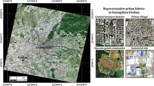
As a highly developed area, the Guangzhou-Foshan metropolitan area features a high diversity of urban fabrics (Chen et al. 2017c; Taubenböck et al. 2014; Tian, Liang, and Zhang 2017), such as the high-rise urban form in the central business district, the crowded multi-story buildings in the heavily populated “urban villages,” the low-density upscale gated communities, the concentration of large low-rise metal roofed buildings in industrial sites, and so on (Figure 1). Therefore, the Guangzhou-Foshan metropolitan area is an adequate testbed to evaluate our method that aims at delineating urban form types.

2.2. Data sources and pre-processing

The main research data is a 2m resolution remote sensing image derived by the Ziyuan-3 (ZY-3) satellites (Li, Wang, and Jiang 2021; Huang, Yang, and Yang 2021) (Figure 1). The image acquisition date is 14 April 2015. The selected image covers the Guangzhou-Foshan metropolitan area and the suburbs as well. We tessellate the image using blocks of 128 × 128 pixels (i.e. 256 m × 256 m per block), resulting in 39,470 blocks in total. The choice of this block size is based on the previous study of image processing for deep learning (Lerouge et al. 2015), and also aims to approximate the average size of local neighborhoods. The subsequent analysis of urban forms and functions is thus at the level of image blocks. In addition to the ZY-3 image, a Synthetic Aperture Radar (SAR) image derived by the Sentinel-1A satellite is also used. This is mainly because SAR images can capture and represent the building height information (Li et al. 2020a; Guida, Iodice, and Riccio 2010). The SAR image we selected was acquired on 15 June 2015. The spatial resolution of the image is resampled to 16 m. We also tesselate the image using the 256 m × 256 m blocks (Table 2).

Table 2. The technical information of dataset and model input requirement

Data sources	Resampled resolution (m)	Input feature type	Number of image blocks	Image block size (m^2)	Input size (pixels)
ZY-3	2	MBI	39,470	256 × 256	128 × 128
Sentinel-1 A	16	SAR	39,470	256 × 256	16 × 16

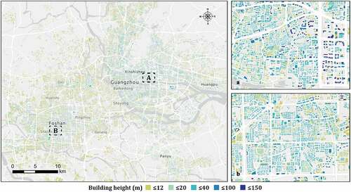
Furthermore, a dataset of building footprints is created using the Application Programming Interface (API) of Baidu Maps. This dataset provides the location, spatial coverage, and height for each individual building (Figure 2), which is useful to infer urban form types. Another two data sets, i.e. the POIs and the Tencent User Density (TUD) data, are used for urban functions analysis. The POIs data provide information on activity types (Li et al. 2022, 2021b), while the TUD data represent the intensity of urban activities. The POIs data are collected from Baidu Maps in 2015, representing the locations where five representative activity types take place: residence, office, shopping centers, hotel, and factory. The TUD data provide hourly location records of Tencent social media users. Since Tencent is the biggest social media platform in China, the TUD data are considered as an appropriate proxy of urban activity intensity. The hourly TUD data span from June 15 to 21, 2015, with 25-m resolution.

Figure 2. Building footprints data with the height attribute. Panels A and B are the zoom-in views of building footprints in two representative places.

2.3. Methods

As shown by Figure 3, we first tessellate the ZY-3 image and the Sentinel-1A SAR image into blocks of 256 × 256 m. Here, the Sentinel-1A SAR image blocks are used to enhance the information related to building height. We then calculate the Morphological Building Index (MBI) for each ZY-3 image block to highlight the distribution of buildings (Section 2.3.1). Then, we use MRCAE to transform the image blocks into urban vectors (i.e. urban form features) (Section 2.3.2). With these vectors, we sequentially apply Self-Organizing Map (SOM) and Gaussian Mixture Model (GMM) to group the image blocks into several urban form types (Section 2.3.3). Finally, we use the auxiliary data, including building footprints, POIs, and the TUD data, to analyze the physical and functional properties of each urban form type (Section 2.3.4).

Figure 3. The technical procedure for the extraction of urban form types and their properties.

2.3.1. MBI

MBI is an effective approach to strengthen the information of buildings in high-resolution remote sensing images (Huang and Zhang 2011). Buildings usually have high local contrasts in remote sensing images because of the relatively high reflectance of roofs. Therefore, the MBI calculation is based on the brightness values of image pixels. In our analysis, after tessellating the image into image blocks, each of the input image blocks is first converted to brightness values:

(1) $b(x)=\underset{1\le k\le K}{max}(M_k(x))$(1)

where $b\left(x\right)$ is the brightness of pixel $x$, and $M_k\left(x\right)$ is the spectral value of pixel $x$ at $k^{th}$ band. Next, the brightness values of each image block are reconstructed using Top-Hat Transformation (THR) (Soille 2013), which is defined as the difference between an input image and its morphological opening result:

(2) $TH{R}^{s,dir}(b)=b-{\gamma }_{RE}^{s,dir}(b)$(2)

where $TH{R}^{s,dir}\left(b\right)$ is the result of top-hat transformation for image block $b$, and ${\gamma }_{RE}^{s,dir}\left(b\right)$ is the morphological opening operation for image block $b$. The superscripts $s$ and $dir$ refer to the size and direction, respectively, of a linear Structural Element (SE) in the reconstruction. Here directions ($dir$) of 45°, 90°, 135°, and 180° are selected, as suggested by Huang and Zhang (2011). The THR values can reflect the difference of brightness between buildings and their neighborhood within the region of the SE. As buildings are relatively isotropic and have high THR values in all directions, an average operator is then used to integrate the multidirectional THR:

(3) ${\overline{THR}}^s\left(b\right)=\underset{dir}{\mathrm{m}\mathrm{e}\mathrm{a}\mathrm{n}}\left(TH{R}^{s,dir}\left(b\right)\right)$(3)

The multiscale THR on Differential Morphological Profiles (DMP) is needed to be calculated because buildings in high-resolution images have various spatial patterns with different shapes, sizes, and heights. It can be obtained by changing the SE size of THR at a regular interval.

(4) $TH{R}_{DMP}^s=|{\overline{THR}}^{s+\mathrm{\Delta }s}(b)-{\overline{THR}}^s(b)|$(4)

where $\mathrm{\Delta }s$ is the interval of the SE size. Here, the size range of SE is (2, 72) at intervals of seven. Then, the mean value of the multiscale THR is taken as MBI:

(5) $MBI=\underset{s}{mean}TH{R}_{DMP}^s$(5)

More details of the MBI calculation can be found in Huang and Zhang (2011).

The resulting MBI images are further transformed using a power-function with the transform parameter $\gamma$ set as 1.5:

(6) $PT(MBI)=c\times (\frac{MBI}{c}{)}^{\gamma }$(6)

where $PT$ is the power transformation function, $c$ is the maximum value in the MBI images. This procedure is used to reduce the interference of image blocks with low MBI values in the subsequent network training. By this means, the building information in each image block can be strengthened, thereby facilitating the subsequent generalization of urban form types. Finally, the values of all pixels are linearly rescaled to the range of (0, 1). The rescaled MBI image blocks are used to train a CAE at the next step.

2.3.2. MRCAE

In our analysis, we modify the conventional CAE structures by adding the ASPP structure and the shortcut connections, thereby forming a new network architecture called MRCAE (Figure 4(a,b)). First, we use an ASPP structure (Chen et al. 2018) in order to extraction of the multiscale features from the input images (Figure 4(e)). ASPP is the combination of atrous convolution and Spatial Pyramid Pooling (SPP). Here, the atrous convolution (Supplementary Figure S1), which operates by changing the resolution of features and adjusting the convolution filters’ field-of-view, favors the extraction of image information at a larger scale (Chen et al. 2017a). On the other hand, SPP captures different ranges of image contexts through replacing the conventional pooling layers with the pooling windows of different sizes (He et al. 2015).

Figure 4. (a) A conventional structure of CAE. (b) The structure of encoder used in the proposed MRCAE. The red arrows on the edge represent shortcut connections. (c) The structure of the decoder, which can be connected to the end of the architectures shown in (a) and (b). (d) The detailed feature fusion module. (e) The detailed structure of ASPP.

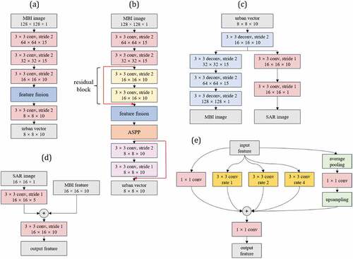
ASPP implements the atrous convolution with multiple atrous rates to replace the pooling windows in SPP whereby the outputs of the encoder can generate multiscale features without reducing the spatial resolution. In our analysis, we use atrous convolutions with the rates of 1, 2, and 4 (Chen et al. 2017b), and a 1 × 1 convolution layer (Figure 4(e)). To incorporate the global context information, we adopt the operations suggested by Chen et al. (2017), which include the average pooling of image-level features, and the 1 × 1 convolution and upsampling operations. In the end, another 1 × 1 filter is used to integrate the features of all scales.

The second modification of the proposed MRCAE is the use of the shortcut connections. A shortcut connection (Figure 4(b)) is to skip one or more layers and transmit the updated information from the high-level network to the low-level network through identity mapping. The network layers that are linked by the shortcut connections are called the residual block, as shown in Figure 4(b). By adding a few residual blocks, the network becomes deeper and performs better while avoiding the problems of vanishing/exploding gradient and degradation (He and Sun 2015; He et al. 2016; Li et al. 2021a). In the proposed MRCAE, we add two residual blocks to increase the depth of the network (Figure 4(b)).

We also design a feature fusion module to aggregate the features of the MBI images and the SAR images, as illustrated by Figure 4(d). We first use a 3 × 3 convolution layer to extract SAR image features. These features are then concatenated with the MBI features and forwarded together to another 3 × 3 convolution layer for the aggregation of these two different kinds of features. After the feature fusion procedure, the ASPP module is implemented to capture the multiscale information of building distribution and height. As shown in Figure 4(c), we use two 3 × 3 convolution layers after the first deconvolution layer to restore SAR images in the decoding network.

The full network architecture is shown in Figure 4(b,c). The convolution layers and the transposed convolution layers are used to construct the encoder and decoder, respectively. We set the stride to two in the convolution layers (and the transposed convolution layers as well) to achieve the same effects of the max-pooling layer and the up-sampling layer. Batch normalization, which refers to the normalization of the inputs to a layer for each mini-batch, is applied after each convolution operation to speed up network convergence (Ioffe and Szegedy 2015). Here mini-batch means that only a subset of training data instead of the full set are used to update the parameters in each iteration, which is a prevalent strategy for faster convergence. The commonly used Relu function is selected as the activation function. The loss function is based on the Mean Square Error (MSE) between the restored and the input images:

(7) $\mathcal{L}=\frac{1}{N}\sum _i^N\left({\parallel M_i}^{\prime }-M_i{\parallel }_2^2+\lambda \parallel {S_i}^{\prime }-S_i{\parallel }_2^2\right)$(7)

where $M$ and $M{ }^{\mathrm{\prime }}$ are the input and restored MBI images, respectively. $S$ and $S{ }^{\mathrm{\prime }}$ are the input and restored SAR images, respectively. $\lambda$ is a hyperparameter used to determine the MSE weights of MBI and SAR images. We consider building distribution and building height both take the same contribution to urban form. Therefore, $\lambda$ is set to 1 in our experiment. Adaptive Moment Estimation (Adam) (Kingma and Ba 2014) is selected as the optimization algorithm to minimize the loss function.

We implement the proposed network using the library of PyTorch 1.8.1 in Python 3.8. We set the batch size of the input images as 32 mainly according to the limitation of our Graphics Processing Unit (GPU) memory (10 GB). We train our models from scratch for 100 epochs until convergence. As suggested by Kingma and Ba (2014), we set the learning rate as 0.001 and the exponential decay rates as default.

Before the training, all image blocks are divided into three sets for training, validation, and testing with ratios of 64%, 16%, and 20%, respectively. After the training is finished, each MBI image block is transformed by the encoder into features with a size of 8 × 8 × 10. Here, the size of features is set according to a previous encoder experiment that yielded satisfactory results using global urban data (Moosavi 2017). The features are further flattened to a one-dimensional vector with a length of 640 (8 × 8 × 10 = 640), which store the latent characteristics of urban form in each image block. We refer to them as urban vectors, which are used for urban form clustering.

2.3.3. SOM and GMM

SOM is a kind of artificial neural network that can transform the high-dimensional input data points into a low-dimensional, discretized space while preserving the topology of the input data points (Kohonen 2013). The main superiority of the SOM is that it can support the clustering and visualization of high-dimensional multivariate data (Skupin and Hagelman 2005; Ling and Delmelle 2016). The output space consists of a set of connected nodes, each represented by a weight vector. Each input data point is assigned to one of the nodes, and each weight vector can be regarded as the general feature of all data points assigned to this node. In our analysis, the SOM as a pre-clustering process is used to handle the complex urban vectors and generalize urban form types.

A SOM model is composed of an input layer and a competition layer. The competition layer, which also is the output space of a SOM, is usually a two-dimensional square grid of nodes. According to empirical literature (Tian, Azarian, and Pecht 2014), the side length of the square grid can be set as $\sqrt{5\times \sqrt{N}}$, where N refers to the total number of data points and is 39,470 in our case. As a result, the side length of the square grid in the competition layer is 32, and the total number of nodes is 1024 (32 × 32). Each node in the competition layer will represent a cluster of input data. During the training, the similarity between the input vectors and the weights of each node is measured using Euclidean distance. Then, the node that is most similar to the input vectors is selected and regarded as the Best Matching Unit (BMU). After that the weights of the BMU and its neighboring nodes in the competition layer are adjusted toward the input vectors. Therefore, an important feature of SOM is that similar data points will be assigned to nodes close to each other, while dissimilar data points will be located in nodes far from one another in the grid.

The SOM nodes are usually applied to a certain clustering method to reveal the patterns of input data (Skupin and Hagelman 2005). In our case, the trained SOM will yield up to 1024 clusters of urban vectors, which are difficult to analyze and interpret. Therefore, to further generalize the results, we implement GMM to cluster the SOM nodes. The GMM clustering results will be the final label of the data points (image blocks) in each node. GMM assumes that the input data follow Gaussian distribution, and, therefore, the distribution of the input data can be regarded as a mixture of many unimodal Gaussian distributions. After setting the number of unimodal Gaussian distributions, denoted as $k$, GMM can divide the entire data set into different groups that correspond to the specified number of Gaussian distributions. The selection of $k$ is based on the Bayesian Information Criterion (BIC). The lower BIC scores, the better performance is the model to fit the distribution of the input data (Wit, Heuvel, and Romeijn 2012). Generally, BIC scores decrease as $k$ increases. This is straightforward because the use of more individual distributions can better fit the distribution of the input data, although the risk of overfitting also increases when increasing the value of k. To avoid this problem, we determine the value of k according to the difference of the BIC scores. The difference reflects to what extent the performances between two consecutive values of $k$ (i.e. $k$ vs. $k-1$). The reasonable setting of $k$ can be found once the difference of BIC scores plateau, which indicates that there is no much gain by increasing k.

2.3.4. Interpretation of urban form types and their functions

The interpretation of the clustering results has two procedures. The first procedure is to understand what those urban form clusters are according to their physical properties. Three indicators are used to characterize the resulting urban form clusters, including mean building density, mean building height and mean nearest neighbor distance. Specifically, for an urban form cluster $c$, its mean building density is the mean building count of all image blocks in c. Similarly, mean building height is the mean height overall image block in $c$. To acquire the mean nearest neighbor distance for $c$, the nearest neighbor distance is first calculated at the building level in each image block. Then, the mean nearest neighbor distance for each image block is calculated. Finally, the mean nearest neighbor distance for c is calculated as the mean of the block-level mean nearest neighbor distance.

The second procedure is to understand the functional properties of the resulting urban form clusters in terms of the composition of function types and activity intensity. To characterize the function composition, we apply the Enrichment Factors (EF) (Chen et al. 2017c; Verburg et al. 2004) to a set of POIs that represent the typical function types in a city:

(8) $E{F}_{i,l}=\frac{n_{l,i}/n_i}{N_l/N}$(8)

where $E{F}_{i,l}$ denotes the enrichment of POIs in the $l^{th}$ category in the $i^{th}$ unit (e.g. a block and an entire urban form cluster, depending on the enrichment of POIs in what kinds of units we want); $n_{l,i}$ is the number of POIs in the $l^{th}$ category located in the unit; $n_i$ is the number of blocks in the $i^{th}$ unit; $N_l$ is the total number of POIs in the $l^{th}$ category; and $N$ is the total number of POIs in the entire study area. Therefore, for unit $i$, $E{F}_{i,l}$ is a comparison of the abundance of POIs in the $l^{th}$ category against the global average. A larger $E{F}_{i,l}$ value indicates that POIs of the $l^{th}$ category are more concentrated in the $i^{th}$ unit. If $E{F}_{i,l}$ > 1, the concentration is more pronounced in the $i^{th}$ unit than the regional average, and vice versa.

Additionally, EF is also applied to analyze the spatial transition of urban form clusters. We delineate the buffer zones of city centers using the distance interval of 1500 m and assess the richness of urban form clusters in each buffer zone by calculating EF. In this case, $n_{l,i}$ is the area of urban form cluster $l$ in the $i^{th}$ buffer ring, $n_i$ is the total urban area in the $i^{th}$ buffer ring, and $N_l$ and $N$ are the total areas of urban form cluster $l$ and all urban form clusters, respectively.

The activity intensity of each urban form is measured using the TUD data. First, for each block, the mean TUD at each hour is calculated. Second, for each urban form cluster, the block-level mean TUD values at each hour are aggregated by averaging. Finally, the temporal curves of TUD for each urban form cluster are plotted to interpret their functional characteristics.

3. Implementation and results

3.1. MRCAE evaluation

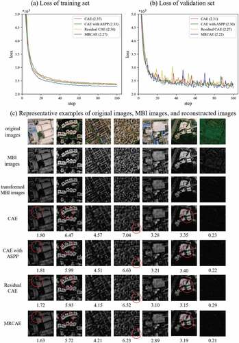
We first evaluate four CAE models, including the original CAE, CAE with ASPP, residual CAE (i.e. CAE with residual blocks), and MRCAE, to highlight the effectiveness of MRCAE in restoring the information of input images. To assess the uncertainty of the proposed method, we randomly divide our input data into training, evaluation, and test set several times, then repeatedly run the experiments. By this means, we obtain 30 outcomes for each model. Figure 5 shows the example of the loss function curves of the four CAE models for both the training and validation sets. The results reveal that the performances of the CAE models integrated with either an ASPP structure or the residual blocks are only slightly better than that of the standard CAE model. However, if both the ASPP structure and the residual blocks are combined (i.e. MRCAE), the improvement in model performance is much more evident. The overall testing error for the MRCAE model (MSE = 2.22 ± 0.08) is the smallest compared with those for the conventional CAE (MSE = 2.28 ± 0.08), CAE with ASPP (MSE = 2.25 ± 0.10), and residual CAE (MSE = 2.25 ± 0.07). The representative examples of the reconstructed images by the four CAE models are shown in Figure 5(c). By visually inspecting these examples, one can find that the results yielded by the MRCAE model have less noise than the results of the other three models.

Figure 5. (a) and (b) are the four CAE models’ loss function curves using the training and validation sets, respectively. The numbers in the legend represent the minimum average MSE in 100 epochs during the training or validation. (c) Representative examples of the reconstructed images generated by the four CAE models. The numbers below the images are the values of MSE. The units of the values are 1 × 10⁻³.

3.2. Urban form clustering

As we mentioned in Section 2.3.3, after SOM training we can get 1024 SOM nodes each represented by a weight vector. We can use the weight vector of each node to represent the urban form features of all the image blocks assigned to this node. The length of a weight vector is the same as any input urban vector. Therefore, we can decode the weight vector of each node by using the MRCAE’s decoder to find out the visual features of its image block members. Figure 6 shows the decoded weight images of seven representative nodes and their image block members. The resulting grid of the trained SOM is ordered spatially in such a way that similar nodes are close to each other (Figure 6(a)). Although the images of the decoded weights are not straightforward to recognize and understand, they in effect have captured the important features of the image block members (Figure 6(b)). The weights have revealed the distribution, density, and spatial layout of the buildings. Here, the red area of the decoded weights (Figure 6(a)) corresponds to the presence of highly urbanized image blocks, while the blue areas refer to the sub-urban areas that have less buildings.

Figure 6. (a) The resulting grid of the trained SOM with similar nodes being close to each other. Here the red area corresponds to the highly urbanized image blocks, while the blue areas represent the sub-urban areas that have fewer buildings. The green box, purple box, and the aqua green boxes correspond to nodes that represent sub-urban areas, highly urbanized areas, and urban areas with low building density. (b) The decoded images of seven representative nodes and their image block members. A and B represent highly urbanized areas. C, D, and E represent urban areas with low building density. F and G represent waterfront areas..

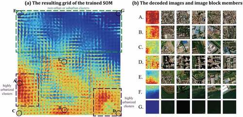
As shown in Figure 6, the nodes in the upper half of the grid represent sub-urban or non-urban areas (i.e. the nodes within the green box), while those in the lower half represent urbanized areas with more buildings. The nodes in the lower-left side and lower-right corner of the grid (i.e. the nodes within the purple box) correspond to image blocks that have high MBI values. They represent highly urbanized areas. The nodes in the lower center of the grid (i.e. the nodes within the aqua green boxes) correspond to urban areas with relatively low building density. Several representative image blocks are shown in Figure 6(b). The image blocks in the rows A and B of Figure 6(b) are examples of compactly built areas, which are almost fully covered by buildings. The image blocks in the rows C, D, and E are examples of urban areas with low building density and demonstrate similar spatial compositions and orientation. The image blocks in the row F represent building distribution in sub-urban areas. For any image block in this example, buildings are detected only in less than half of an image block, while the remaining part is the non-built area. Overall, the trained SOM can capture important information that distinguishes urban forms from one type to another.

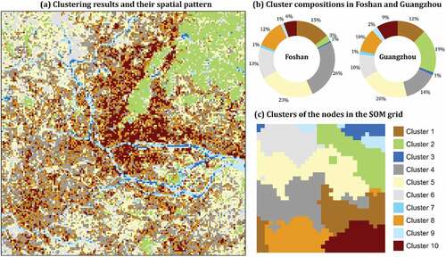
As the resulting SOM grid nodes are still too many to interpret, the GMM method is applied to the 1024 nodes to reduce the number of clusters. The different choices of cluster numbers are evaluated using the BIC scores and their gradient. Supplementary Figure S2(a) and (b) show the results of BIC scores and their gradient, respectively. According to the gradient, the gain of improvement reduces when the number of clusters increases and becomes stable at the cluster number of 10. Therefore, the final choice of cluster number is 10 for urban form clustering. Figure 7 shows the results of urban form clustering in both the geographical space and the SOM grid. By mapping the 10 urban form clusters to the SOM grid (Figure 7(c)), one can easily recognize that these clusters are basically the aggregation of neighboring nodes, mainly because the arrangement of a SOM grid is that similar nodes are close to each other.

Figure 7. The clustering results generated by GMM. (a) Distribution of urban form clusters in the geographical space. (b) Cluster compositions in Foshan and Guangzhou. (c) Distribution of urban form clusters in the SOM grid.

3.3. Physical and functional properties of each urban form cluster

The physical properties of each urban form cluster are acquired by analyzing the building footprints data. Table 3 explains the classification schemes for the resulting clusters according to the physical properties of mean nearest neighbor distance, mean building height, and mean building density. Each urban form cluster is named by the combination of classes (Table 4), such as Open low-rise with medium density (cluster #5). Figure 8 demonstrates the representative examples of each urban form cluster, and Table 4 summarizes the physical properties of each urban form cluster.

Figure 8. The representative examples of the resulting urban form cluster. The names of these clusters are interpreted according to the mean nearest neighbor distance, building height, and density.

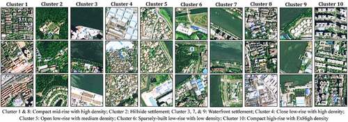
Table 3. The classification schemes of urban form clusters

Mean nearest neighbor distance (m)	Class	Mean building height (m)	Class	Mean building density	Class
<11	Compact	<11	Low-rise	<9	Low
11–15	Close	11–14	Mid-rise	9–12	Medium
15–26	Open	>14	High-rise	12–31	High
> 26	Sparsely-built			<31	ExHigh

ExHigh = Extremely high. The cutoff points are determined using the natural breaks method.

Table 4. The physical properties and image examples of each cluster (standard deviations are shown in the brackets)

Cluster	Mean nearest neighbor distance	Mean building height	Mean building density	Cluster name
1	9.94 (23.54)	12.69 (11.70)	30.25 (40.25)	Compact mid-rise with high density (+)
2	36.24 (64.60)	8.34 (11.43)	6.09 (8.02)	Sparsely-built low-rise with low density (Hillside settlement)
3	13.80 (22.32)	9.60 (11.07)	6.95 (10.14)	Close low-rise with low density (Waterfront settlement I)
4	13.58 (35.33)	10.29 (9.21)	28.21 (42.94)	Close low-rise with high density
5	25.41 (65.90)	9.15 (10.23)	11.87 (18.65)	Open low-rise with medium density
6	32.20 (62.53)	7.86 (8.04)	8.02 (11.47)	Sparsely-built low-rise with low density
7	19.85 (36.95)	11.01 (17.76)	5.95 (7.87)	Open mid-rise with low density (Waterfront settlement II)
8	10.21 (24.21)	12.51 (11.67)	29.07 (39.04)	Compact mid-rise with high density (-)
9	20.55 (48.15)	12.15 (15.75)	11.33 (15.68)	Open mid-rise with medium density (Waterfront settlement III)
10	7.65 (17.11)	17.73 (15.42)	37.79 (46.88)	Compact high-rise with ExHigh density

ExHigh = Extremely high.

For clusters #1 and #8, they share similar physical properties and hence both of them are classified as compact mid-rise with high density. Despite that, the major differences between clusters #1 and #8 lie in the morphology. As illustrated by the SOM grid in Figure 7(c), cluster #1 and cluster #8 are located in different parts of the grid, in which cluster #1 is in the left of cluster #10 and cluster #8 is on the top of cluster #10. With Figure 6(b), one can easily identify the different building layouts in the two regions that cluster #1 and cluster #8 cover. Nevertheless, an additional “+” sign is assigned to cluster #1 because cluster #1 has slightly shorter neighboring building distance, greater heights, and higher density than cluster #8. Similarly, clusters #2 and #6 are referred to as sparsely built low-rise with low density. However, cluster #2 covers the settlements that are built on the hillside, while cluster #6 includes low-rise buildings that are in the flatland. For clusters #3, #7, and #9, although they are different in terms of building characteristics (Table 4), they consistently belong to settlements along the waterfront, with cluster #3 featuring low-rise buildings and clusters #7 and #9 featuring mid-rise buildings. Clusters #4 and #5 are also low-rise urban forms. They collectively cover more than 38% of the study area, which are the two largest clusters in terms of the areal fractions. Cluster #10 is distributed mainly in the core of the Guangzhou-Foshan metropolitan area (Figure 7), with the shortest neighboring building distance, the tallest buildings, and the greatest density as compared to other clusters.

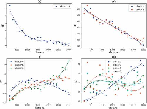
To understand the spatial transitions of the resulting urban form clusters, buffer zones of the city center are delineated using the distance interval of 1500 m (see Figure 1 for the locations of the two city centers). In each buffer zone, the abundance of a certain urban form cluster is measured using EF (Equation (6)(6) $PT(MBI)=c\times (\frac{MBI}{c}{)}^{\gamma }$(6) ). Figure 9 plots the spatial trends of EF values for all urban form clusters. The only high-rise urban form cluster (#10) demonstrates an evident downward trend of EF from the city center to the urban periphery (Figure 9(a)). The abundance of cluster #10 rapidly declines from the city center and reaches less than 1.0 after the buffer distance range of 12–16 km. The two compact mid-rise clusters (#1 and #8) show similar declining trends of EF values outward from the center of the city, although their trends are more linear than that of cluster #10 (Figure 9(b)). The three low-rise clusters (#4, #5, and #6), however, show relatively different trends (Figure 9(c)). The abundance of cluster #4 first gradually increases within the 12 km from the city center and slowly declines afterward. Clusters #5 and #6 consistently show the monotonous upward trends of abundance, although the abundance of cluster #6 increases more rapidly than cluster #5 after the buffer distance of 20 km. The spatial distribution of waterfront settlements (clusters #3, #7, and #9) relates mainly to rivers and lakes and hence their EF values show no relationships with the distance to city center (Figure 9(d)). While the mountainous areas are in the urban periphery (Figure 1), the spatial trend of the abundance of hillside settlement (cluster #2) is similar to those of the low-rise clusters (Figure 9(c)).

Figure 9. The spatial transition of urban form clusters from the city center. The y-axis indicates the EF values of urban form clusters in different buffer zones of the city center.

The functional properties of all urban form clusters are analyzed using POI and TUD data, of which the former reflects major activity composition while the latter represents activity intensity. For the five POI types, EF calculation is applied for each urban form cluster (Table 5). Additionally, the temporal profiles of mean TUD for each urban form cluster are summarized (Figure 10).

Figure 10. The temporal TUD profiles in hours for all urban form clusters.

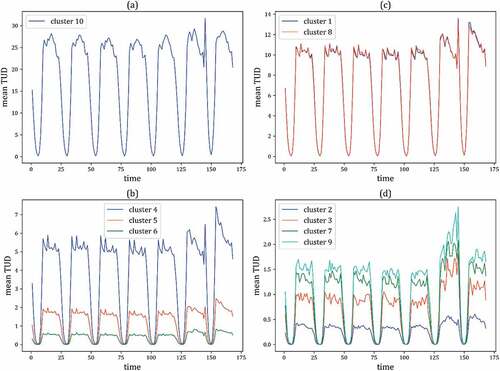
Table 5. The EF of POIs for each urban form cluster

Cluster	Factory	Hotel	Mall	Office	Residence
1	1.10	0.98	1.02	0.84	0.96
2	1.10	1.42	0.68	0.58	0.73
3	0.88	1.43	0.98	0.00	1.39
4	1.58	0.75	0.92	0.54	0.70
5	1.66	0.79	0.55	0.38	0.74
6	1.81	0.83	0.21	0.35	0.55
7	1.06	1.14	0.00	0.27	1.48
8	1.07	0.92	0.91	0.99	1.01
9	0.83	0.97	0.36	0.74	1.64
10	0.48	1.22	1.17	1.46	1.21

As shown by Table 5, the 10 urban form clusters show substantial differences in the composition of urban functions. The activity of industrial production concentrates in three low-rise urban form clusters, including clusters #4, #5, and #6, as they have the highest EF values of factory POIs. Notably, the collective proportion of these three urban form clusters in Foshan is as high as 62% (Figure 7(b)), mainly because manufacturing is at the heart of Foshan’s economy (more than 56% of GDP). Moreover, the building density levels are strongly correlated with the activity intensity within these three clusters. Cluster #4 has greater building density than clusters #5 and #6 and has a greater activity intensity than the other two low-rise clusters as well (Figure 10(c)). In addition, the activity profile of cluster #4 shows two evident peaks on Saturday and Sunday, partly because of the relatively greater abundance of shopping malls than the other two low-rise clusters (Table 5). The two compact mid-rise clusters (#1 and #8) show almost identical intensity profiles (Figure 10(b)). These two clusters consistently feature a relatively high concentration of industrial activities. Despite that, some differences still exist in the composition of other functions: Cluster #1 has greater abundance of malls while cluster #8 has greater abundance of offices (Table 5).

For the hotel POI, which relates to activities of business travel and touring, it is most abundant in the urban form types of hillside settlement (cluster #2), waterfront settlements (clusters #3 and #7), and compact high-rise form (cluster #10). This result reflects two different location preferences of hoteling, i.e. for better scenic views (clusters #2, #3, and #7) and for better accessibility (cluster #10). As depicted by Figure 10(d), the activity intensity of clusters #2, #3, #7, and #9, consistently reach the highest levels at the weekend, probably due to the increase in touring and hoteling activities. In addition to the concentration of hoteling activity, cluster #10 also features the concentration of malls and offices. This is easy to understand because the developments of malls are strongly influenced by density, while office-based businesses are also attracted to high-density areas that would increase job accessibility and create other benefits such as scale economy and cooperation. For residential areas, however, they concentrate in urban form clusters that have better scenic views or better proximity to jobs and services, such as the clusters of waterfront settlement (#3, #7, and #9) and the compact high-rise cluster (#10).

3.4. Method comparison

We carry out additional experiments to evaluate and compare the performances of the original CAE model, MRCAE model, and several other conventional image feature extraction methods. Here, we use Grey Level Co-occurrence Matrices (GLCM) (Soh and Tsatsoulis 1999) and Histograms of Oriented Gradients (HOG) (Dalal and Triggs 2005) to represent building features and further apply KMeans and GMM for clustering. In addition, we also evaluate our approach by directly applying GMM to the MRCAE urban vectors.

The aim of the comparison experiments is to explore to what extent the different features (or latent representations) generated by the selected methods of image feature extraction can influence the results of urban form clustering. However, it is difficult to directly compare urban vectors because they are in different domains. While all of these vectors are for urban form clustering, it is feasible to evaluate them by comparing the final clustering results. To this end, we use the Geodetector Q-statistic (Wang et al. 2010) that measures how well a categorical map can explain the spatial pattern of a geographical attribute. More specifically, we use the Q-statistic to evaluate how well the resulting urban form maps can explain the spatial patterns of building attributes, including building height and building area. The values of the Q-statistic range from 0 to 1, and a higher value of the Q-statistic indicates better performance of the urban form map. The calculation of the Q-statistic is also provided in the supplementary information.

As shown by Table 6, the clustering results based on the conventional CAE can explain 53% and 52% of the spatial distributions of building height and building area, respectively. The MRCAE model further improves the results by 2.1% and 3.3% in terms of explaining building height and building area, respectively. However, if we directly apply GMM to the urban vectors extracted by MRCAE, the corresponding q-statistic values are only 0.45 and 0.43. These results confirm the significance of SOM. The urban form clustering results obtained from the selected unsupervised methods consistently yield low q-static values. Nevertheless, with the same input features, the results of GMM are better than those of KMeans. The results also suggest that the clustering results using the HOG features are better than those using the GLCM features. Surprisingly, if the GLCM features and the HOG features are combined, the results are worse than those only using the HOG features.

Table 6. Comparison of the Geodetector Q-statistic for t results of urban form delineation obtained from the CAE-SOM-GMM, MRCAE-SOM-GMM, MRCAE-GMM, GLCM-GMM, HOG-GMM, GLCM+HOG-GMM, GLCM-KMeans, HOG-KMeans, and GLCM+HOG-KMeans

	CAE-SOM-GMM	MRCAE-SOM-GMM	MRCAE-GMM	GLCM-GMM	HOG-GMM	GLCM+HOG-GMM	GLCM-KMeans	HOG-KMeans	GLCM+HOG-KMeans
$q_{bh}$	0.530	0.551	0.449	0.427	0.466	0.459	0.367	0.435	0.412
$q_{ba}$	0.519	0.552	0.427	0.455	0.488	0.499	0.391	0.448	0.417

Q_bh = q-statistic of building height, q_ba = q-statistic of building area.

4. Discussion

Consistent classification of urban form can facilitate the understanding of how urbanization interacts with climate change. Conventional approaches of supervised classification require a rigidly defined scheme of urban form classes and high-quality sample data with class labels. Due to the complexity of urban systems, it is challenging to consistently define urban form classes and collect metadata to describe these classes (Eldesoky, Gil, and Pont 2021). Uncertainty arise from the inaccurately or inconsistently labeled training data may reduce the reliability of urban form classifications (Zhang, Du, and Zheng 2020). While the unsupervised deep learning approaches can avoid the problems mentioned above, they have not yet been well examined in the generalization of urban form types. A previous study had demonstrated the effectiveness of unsupervised deep learning in capturing the inherent similarity of urban street structures at local scales (Moosavi 2017). In our analysis, however, we developed a new architecture of autoencoder, namely the MRCAE, to delineate urban form types from the perspective of building layout using a high-resolution remote sensing image. The contribution of our work is therefore twofold: (1) our case study has demonstrated that it is feasible to learn urban form types directly from unlabeled data using high-resolution remote sensing images and (2) our study contributes methodologically with the proposed MRCAE that outperforms the conventional CAE models in the generation of deep features for images, which is important to clustering analysis and image classification as well.

The resulting urban form types are essential to help quantify the environmental impacts of urbanization. For instance, an immediate usage of urban form classification is to analyze the thermal behavior of different types of urbanization at neighborhood scales (Choudhury, Das, and Das 2021). Scenario simulations can then be implemented to trade-off the benefits of, for example, heat island mitigation gained by changing urban form and its economic costs (Despini et al. 2021; Khamchiangta and Dhakal 2021). Additionally, maps of urban form types also pertain to the input data of urban climate models such as the Urban Canopy Models (UCMs) (Masson et al. 2020). The presented spatial results of urban form types can further become a basis to refine and distinguish the setting of UCM parameters (e.g. sky view factor, mean building height, albedo, roughness, etc.) in different urban form types, thereby introducing the urban heterogeneity to help understand the climate response of future urbanization. A recent study has demonstrated that refining the UCM parameters can bring promising improvements to the simulations of wind and air temperature in highly urbanized areas (Chen et al. 2021).

While urbanization leads to increased imperviousness and human activities, which modify the urban heat balance (Guha et al. 2020; John et al. 2020), their impacts can be mitigated by other urban elements such as vegetation and water. In particular, the effective planning and use of “Green Infrastructure (GI)” as a means to improve urban life has gained increasing attention (Fuentes, Tongson, and Viejo 2021). GI refers to parks, water bodies, trees, and other vegetation systems that can help mitigate Urban Heat Islands (UHIs) (Santamouris 2015). Although our study focuses on the form of impervious areas, which are the source of UHIs, it is worth exploring the combined effects of urban form and GI with regard to UHIs in future research. As urban climate cannot be independently explained by individual factors, it is necessary to integrate the features of GI into urban form analysis for a holistic understanding of climate phenomena such as UHIs. To this end, fine and accurate land cover information of GI should be incorporated. The deep learning methods that map urban form using remote sensing images can also be modified and adapted to detect GI objects such as trees, grassland, parks, and their composition (Lumnitz et al. 2021). Additionally, likewise with the scheme of urban form classification, it is useful to develop a GI scheme that categorizes the patterns of GIs with respect to their spatial and compositional attributes (Bartesaghi-Koc, Osmond, and Peters 2019). The further integration of urban form and GI schemes thus can facilitate the understanding of the cumulative climate effects of the natural and man-made urban elements. By means of scenario simulations, it is also feasible to assess the performance of different GI types in temperature reduction in those densely built urban areas (Tiwari et al. 2021).

Our approach also suffers several limitations. First, as aforementioned, we mainly determine urban form types according to the spatial distribution, layouts, and heights of buildings, but do not consider the composition of land covers. It may limit the capability of urban forms generalization and also affect its validity. In future research, multi-band or hyperspectral remote sensing images, which contain abundant land cover information (Prins and Niekerk 2021), can be employed to extract the latent representation of land cover layouts and generalize more representative urban form types. Second, we set the image blocks with only one particular size as 128 × 128 pixels, which corresponds to the ground area of 256 m × 256 m. We chose this size according to the previous deep learning applications (Lerouge et al. 2015), for this image size is convenient for the training of deep learning models. By changing the input size of the autoencoder or using a sliding window approach, comprehensive analysis with different spatial units can be carried out in future research to understand the potential impacts of scales. Third, we applied the proposed method in Guangzhou-Foshan, therefore the results only reflect the urban form in this case study area and may not be compatible with other urban areas or existing schemes of urban form classification. Nevertheless, by using data of many urban areas that cover a large spatial scale, a more general scheme of urban forms can be derived using the proposed method. For instance, it is feasible to apply our method to remote sensing data at global scale such that the full spectrum of urban forms and their transition can be captured. In future research, therefore, we will focus on generalizing urban forms using global data and compare them with some existing schemes such as LCZ (Huang, Liu, and Li 2021).

5. Conclusion

Due to the complexity and diversity of urban form, it is challenging to develop a consistent classification system of urban form types in a top-down manner with well-established rules. This study proposed a new method to understand urban form types from the bottom up based on an unsupervised deep learning approach. We developed MRCAE, a novel convolutional autoencoder network, by integrating an ASPP module and residual blocks into the conventional autoencoder structure.

We applied the proposed method in the metropolitan area of Guangzhou-Foshan, China. Compared with the conventional CAE model, the MRCAE developed in this study can reduce the errors of image restoration by 3% (Figure 5). With the MRCAE model, a set of urban vectors were extracted from image blocks. They were further clustered using the SOM and GMM methods to generate 10 types of urban form. The urban form map generated based on the vectors learned by the MRCAE model can explain 55% of the building height distribution and 55% of building area distribution, which are 2.1% and 3.3% higher than those derived from the conventional CAE model, and much more higher than those derived from other unsupervised methods (Table 6). We further examined the inherent functional properties of the resulting urban form types by using POIs data and TUD data. Each identified urban form type reveals significant spatial transition and urban function mixture patterns, which can be related to its physical properties. In future studies, we will try to apply the unsupervised urban form extraction method to obtain more universal urban form types on larger scales, which can provide useful information to help mitigate the impacts of changing climate.

Disclosure statement

No potential conflict of interest was reported by the author(s).

Data availability statement

The data that support the findings of this study are available from the corresponding author upon reasonable request.

Supplemental data

Supplemental data for this article can be accessed online at https://doi.org/10.1080/10095020.2022.2068384

Additional information

Funding

This work is supported by the National Key R&D Program of China [grant number 2019YFA0607201 and 2017YFA0604401]; the National Natural Science Foundation of China [grant number 41871306]; the Guangdong Natural Science Funds for Distinguished Young Scholar [grant number 2021B1515020104]; and the Fundamental Research Funds for the Central Universities [grant number 20lgzd09].

Notes on contributors

Jihong Cai

Jihong Cai is currently working toward the MS degree in cartography and geographical information system with Sun Yat-sen University, Guangzhou, China. His research interests include urban remote sensing, image classification, and semantic segmentation.

Yimin Chen

Yimin Chen received the PhD degree in Cartography and GIScience from Sun Yat-sen University, Guangzhou, China, in 2014. He is currently an Associate Professor with the School of Geography and Planning, Sun Yat-sen University, Guangzhou, China. His research interests include remote sensing and urban analysis, including deep learning, classification, and sematic segmentation.

References

- Bartesaghi-Koc, C., P. Osmond, and A. Peters. 2019. “Mapping and Classifying Green Infrastructure Typologies for Climate-Related Studies Based on Remote Sensing Data.” Urban Forestry and Urban Greening 37: 154–167. doi:10.1016/j.ufug.2018.11.008.
- Budhiraja, B., G. Agrawal, and P. Pathak. 2020. “Urban Heat Island Effect of a Polynuclear Megacity Delhi–Compactness and Thermal Evaluation of Four Sub-Cities.” Urban Climate 32: 100634. doi:10.1016/j.uclim.2020.100634.
- Chen, X.Y., and Y.M. Chen. 2021. “Quantifying the Relationships between Network Distance and Straight-Line Distance: Applications in Spatial Bias Correction.” Annals of GIS 27 (4): 351–369. doi:10.1080/19475683.2021.1966503.
- Chen, Y.M., X.P. Liu, X. Li, X.J. Liu, Y. Yao, G.H. Hu, X.C. Xu, and F.S. Pei. 2017c. “Delineating Urban Functional Areas with Building-Level Social Media Data: A Dynamic Time Warping (DTW) Distance Based K-Medoids Method.” Landscape and Urban Planning 160: 48–60. doi:10.1016/j.landurbplan.2016.12.001.
- Chen, L.C., G. Papandreou, I. Kokkinos, K. Murphy, and A.L. Yuille. 2017a. “Deeplab: Semantic Image Segmentation with Deep Convolutional Nets, Atrous Convolution, and Fully Connected Crfs.” IEEE Transactions on Pattern Analysis and Machine Intelligence 40 (4): 834–848. doi:10.1109/TPAMI.2017.2699184.
- Chen, L.C., G. Papandreou, F. Schroff, and H. Adam. 2017b. “Rethinking Atrous Convolution for Semantic Image Segmentation.” In 2017 IEEE Conference on Computer Vision and Pattern Recognition (CVPR), Honolulu, July 21-26.
- Chen, B.Y., W.W. Wang, W. Dai, M. Chang, X.M. Wang, Y.C. You, W.X. Zhu, and C.G. Liao. 2021. “Refined Urban Canopy Parameters and Their Impacts on Simulation of Urbanization-Induced Climate Change.” Urban Climate 37: 100847. doi:10.1016/j.uclim.2021.100847.
- Chen, L.C., Y.K. Zhu, G. Papandreou, F. Schroff, and H. Adam. 2018. “Encoder-Decoder with Atrous Separable Convolution for Semantic Image Segmentation.” In European Conference on Computer Vision (ECCV), Munich, September 8–14.
- Choudhury, D., A. Das, and M. Das. 2021. “Investigating Thermal Behavior Pattern (TBP) of Local Climatic Zones (Lczs): A Study on Industrial Cities of Asansol-Durgapur Development Area (ADDA), Eastern India.” Urban Climate 35: 100727. doi:10.1016/j.uclim.2020.100727.
- Crooks, A., D. Pfoser, A. Jenkins, A. Croitoru, A. Stefanidis, D. Smith, S. Karagiorgou, A. Efentakis, and G. Lamprianidis. 2015. “Crowdsourcing Urban Form and Function.” International Journal of Geographical Information Science 29 (5): 720–741. doi:10.1080/13658816.2014.977905.
- Dalal, N., and B. Triggs. 2005. “Histograms of Oriented Gradients for Human Detection.” In 2005 IEEE Computer Society Conference on Computer Vision and Pattern Recognition, San Diego, June 20-26.
- Despini, F., C. Ferrari, G. Santunione, S. Tommasone, A. Muscio, and S. Teggi. 2021. “Urban Surfaces Analysis with Remote Sensing Data for the Evaluation of UHI Mitigation Scenarios.” Urban Climate 35: 100761. doi:10.1016/j.uclim.2020.100761.
- Dong, J., L. Li, and D. Han. 2019. “New Quantitative Approach for the Morphological Similarity Analysis of Urban Fabrics Based on a Convolutional Autoencoder.” IEEE Access 7: 138162–138174. doi:10.1109/ACCESS.2019.2931958.
- Eldesoky, A.H., J. Gil, and M.B. Pont. 2021. “The Suitability of the Urban Local Climate Zone Classification Scheme for Surface Temperature Studies in Distinct Macroclimate Regions.” Urban Climate 37: 100823. doi:10.1016/j.uclim.2021.100823.
- Fuentes, S., E. Tongson, and C.G. Viejo. 2021. “Urban Green Infrastructure Monitoring Using Remote Sensing from Integrated Visible and Thermal Infrared Cameras Mounted on a Moving Vehicle.” Sensors 21 (1): 295. doi:10.3390/s21010295.
- Guha, S., H. Govil, N. Gill, and A. Dey. 2020. “Analytical Study on the Relationship between Land Surface Temperature and Land Use/Land Cover Indices.” Annals of GIS 26 (2): 201–216. doi:10.1080/19475683.2020.1754291.
- Guida, R., A. Iodice, and D. Riccio. 2010. “Height Retrieval of Isolated Buildings from Single High-Resolution SAR Images.” IEEE Transactions on Geoscience and Remote Sensing 48 (7): 2967–2979. doi:10.1109/TGRS.2010.2041460.
- He, K.M., and J. Sun. 2015. “Convolutional Neural Networks at Constrained Time Cost.” In IEEE Conference on Computer Vision and Pattern Recognition (CVPR), Boston, June 7–12.
- He, K.M., X.Y. Zhang, S.Q. Ren, and J. Sun. 2015. “Spatial Pyramid Pooling in Deep Convolutional Networks for Visual Recognition.” IEEE Transactions on Pattern Analysis and Machine Intelligence 37 (9): 1904–1916. doi:10.48550/arXiv.1406.4729.
- He, K.M., X.Y. Zhang, S.Q. Ren, and J. Sun. 2016. “Deep Residual Learning for Image Recognition.” In IEEE Conference on Computer Vision and Pattern Recognition, Las Vegas, June 27–30.
- Heiden, U., W. Heldens, S. Roessner, K. Segl, T. Esch, and A. Mueller. 2012. “Urban Structure Type Characterization Using Hyperspectral Remote Sensing and Height Information.” Landscape and Urban Planning 105 (4): 361–375. doi:10.1016/j.landurbplan.2012.01.001.
- Hladík, J., D. Snopková, M. Lichter, L. Herman, and M. Konečný. 2021. “Spatial-Temporal Analysis of Retail and Services Using Facebook Places Data: A Case Study in Brno, Czech Republic.” Annals of GIS: 1–19. Online-First. doi:10.1080/19475683.2021.1921846.
- Huang, X., A.L. Liu, and J.Y. Li. 2021. “Mapping and Analyzing the Local Climate Zones in China’s 32 Major Cities Using Landsat Imagery Based on a Novel Convolutional Neural Network.” Geo-Spatial Information Science 24 (4): 528–557. doi:10.1080/10095020.2021.1892459.
- Huang, X., Q.Q. Yang, and J.J. Yang. 2021. “Importance of Community Containment Measures in Combating the COVID-19 Epidemic: From the Perspective of Urban Planning.” Geo-Spatial Information Science 24 (3): 363–371. doi:10.1080/10095020.2021.1894905.
- Huang, X., and L.P. Zhang. 2011. “A Multidirectional and Multiscale Morphological Index for Automatic Building Extraction from Multispectral GeoEye-1 Imagery.” Photogrammetric Engineering and Remote Sensing 77 (7): 721–732. doi:10.14358/PERS.77.7.721.
- Ioffe, S., and C. Szegedy. 2015. “Batch Normalization: Accelerating Deep Network Training by Reducing Internal Covariate Shift.” In 32nd International Conference on Machine Learning, Lille, July 6–11.
- John, J., G. Bindu, B. Srimuruganandam, A. Wadhwa, and P. Rajan. 2020. “Land Use/Land Cover and Land Surface Temperature Analysis in Wayanad District, India, Using Satellite Imagery.” Annals of GIS 26 (4): 343–360. doi:10.1080/19475683.2020.1733662.
- Khamchiangta, D., and S. Dhakal. 2021. “Future Urban Expansion and Local Climate Zone Changes in Relation to Land Surface Temperature: Case of Bangkok Metropolitan Administration, Thailand.” Urban Climate 37: 100835. doi:10.1016/j.uclim.2021.100835.
- Kingma, D.P., and J. Ba. 2014. “Adam: A Method for Stochastic Optimization.” In The 3rd International Conference on Learning Representations, San Diego, May 7–9.
- Kohonen, T. 2013. “Essentials of the Self-Organizing Map.” Neural Networks 37: 52–65. doi:10.1016/j.neunet.2012.09.018.
- Lehner, A., and T. Blaschke. 2019. “A Generic Classification Scheme for Urban Structure Types.” Remote Sensing 11 (2): 173. doi:10.3390/rs11020173.
- Leng, H., X. Chen, Y. Ma, N.H. Wong, and T. Ming. 2020. “Urban Morphology and Building Heating Energy Consumption: Evidence from Harbin, a Severe Cold Region City.” Energy and Buildings 224: 110143. doi:10.1016/j.enbuild.2020.110143.
- Lerouge, J., R. Hérault, C. Chatelain, F. Jardin, and R. Modzelewski. 2015. “IODA: An Input/Output Deep Architecture for Image Labeling.” Pattern Recognition 48 (9): 2847–2858. doi:10.1016/j.patcog.2015.03.017.
- Li, L. 2019. “Deep Residual Autoencoder with Multiscaling for Semantic Segmentation of Land-Use Images.” Remote Sensing 11 (18): 2142. doi:10.3390/rs11182142.
- Li, L.F., Y. Fang, J. Wu, J.F. Wang, and Y. Ge. 2021a. “Encoder-Decoder Full Residual Deep Networks for Robust Regression and Spatiotemporal Estimation.” IEEE Transactions on Neural Networks and Learning Systems 32 (9): 4217–4230. doi:10.1109/TNNLS.2020.3017200.
- Li, Z.H., L.M. Jiao, B. Zhang, G. Xu, and J.F. Liu. 2021b. “Understanding the Pattern and Mechanism of Spatial Concentration of Urban Land Use, Population and Economic Activities: A Case Study in Wuhan, China.” Geo-Spatial Information Science 24 (4): 678–694. doi:10.1080/10095020.2021.1978276.
- Li, T., Y.L. Liang, and B. Zhang. 2017. “Measuring Residential and Industrial Land Use Mix in the Peri-Urban Areas of China.” Land Use Policy 69: 427–438. doi:10.1016/j.landusepol.2017.09.036.
- Li, B., Y.F. Liu, H.F. Xing, Y. Meng, G. Yang, X.D. Liu, and Y.L. Zhao. 2022. “Integrating Urban Morphology and Land Surface Temperature Characteristics for Urban Functional Area Classification.” Geo-Spatial Information Science: 1–16. doi:10.1080/10095020.2021.2021786.
- Li, Y.F., S. Schubert, J.P. Kropp, D. Rybski, L. Wan, I. Younis, and Z. Cai. 2020b. “On the Influence of Density and Morphology on the Urban Heat Island Intensity.” Nature Communications 11 (1): 1–9. doi:10.1038/s41467-020-16461-9.
- Li, D.R., M. Wang, and J. Jiang. 2021. “China’s High-Resolution Optical Remote Sensing Satellites and Their Mapping Applications.” Geo-Spatial Information Science 24 (1): 85–94. doi:10.1080/10095020.2020.1838957.
- Li, X.C., Y.Y. Zhou, P. Gong, K.C. Seto, and N. Clinton. 2020a. “Developing a Method to Estimate Building Height from Sentinel-1 Data.” Remote Sensing of Environment 240: 111705. doi:10.1016/j.rse.2020.111705.
- Liang, B., and Q. Weng. 2018. “Characterizing Urban Landscape by Using Fractal-Based Texture Information.” Photogrammetric Engineering and Remote Sensing 84 (11): 695–710. doi:10.14358/PERS.84.11.695.
- Ling, C.J., and E.C. Delmelle. 2016. “Classifying Multidimensional Trajectories of Neighbourhood Change: A Self-Organizing Map and K-Means Approach.” Annals of GIS 22 (3): 173–186. doi:10.1080/19475683.2016.1191545.
- Lu, L.L., Q.H. Weng, D. Xiao, H.D. Guo, Q.T. Li, and W.H. Hui. 2020. “Spatiotemporal Variation of Surface Urban Heat Islands in Relation to Land Cover Composition and Configuration: A Multi-Scale Case Study of Xi’an, China.” Remote Sensing 12 (17): 2713. doi:10.3390/rs12172713.
- Lumnitz, S., T.H. Devisscher, J.R. Mayaud, V. Radic, N.C. Coops, and V.C. Griess. 2021. “Mapping Trees along Urban Street Networks with Deep Learning and Street-Level Imagery.” ISPRS Journal of Photogrammetry and Remote Sensing 175: 144–157. doi:10.1016/j.isprsjprs.2021.01.016.
- Masson, V., W. Heldens, E. Bocher, M. Bonhomme, B. Bucher, C. Burmeister, C.D. Munck, T. Esch, J. Hidalgo, and F. Kanani-Sühring. 2020. “City-Descriptive Input Data for Urban Climate Models: Model Requirements, Data Sources and Challenges.” Urban Climate 31: 100536. doi:10.1016/j.uclim.2019.100536.
- Moosavi, V. 2017. “Urban Morphology Meets Deep Learning: Exploring Urban Forms in One Million Cities, Town and Villages across the Planet.” In 2017 IEEE Conference on Computer Vision and Pattern Recognition (CVPR), Honolulu, July 21–26.
- Moudon, A.V. 1997. “Urban Morphology as an Emerging Interdisciplinary Field.” Urban Morphology 1 (1): 3–10.
- Prins, A.J., and A.V. Niekerk. 2021. “Crop Type Mapping Using LiDAR, Sentinel-2 and Aerial Imagery with Machine Learning Algorithms.” Geo-Spatial Information Science 24 (2): 215–227. doi:10.1080/10095020.2020.1782776.
- Qiu, C., M. Schmitt, L. Mou, P. Ghamisi, and X.X. Zhu. 2018. “Feature Importance Analysis for Local Climate Zone Classification Using a Residual Convolutional Neural Network with Multi-Source Datasets.” Remote Sensing 10 (10): 1572. doi:10.3390/rs10101572.
- Santamouris, M. 2015. “Regulating the Damaged Thermostat of the Cities—Status, Impacts and Mitigation Challenges.” Energy and Buildings 91: 43–56. doi:10.1016/j.enbuild.2015.01.027.
- Skupin, A., and R. Hagelman. 2005. “Visualizing Demographic Trajectories with Self-Organizing Maps.” GeoInformatica 9 (2): 159–179. doi:10.1007/s10707-005-6670-2.
- Soh, L.K., and C. Tsatsoulis. 1999. “Texture Analysis of SAR Sea Ice Imagery Using Gray Level Co-Occurrence Matrices.” IEEE Transactions on Geoscience and Remote Sensing 37 (2): 780–795. doi:10.1109/36.752194.
- Soille, P. 2013. Morphological Image Analysis: Principles and Applications. Berlin: Springer Science & Business Media.
- Stewart, I.D., T.R. Oke, and E.S. Krayenhoff. 2014. “Evaluation of the ‘Local Climate Zone’ Scheme Using Temperature Observations and Model Simulations.” International Journal of Climatology 34 (4): 1062–1080. doi:10.1002/joc.3746.
- Taubenböck, H., M. Wiesner, A. Felbier, M. Marconcini, T. Esch, and S. Dech. 2014. “New Dimensions of Urban Landscapes: The Spatio-Temporal Evolution from a Polynuclei Area to a Mega-Region Based on Remote Sensing Data.” Applied Geography 47: 137–153. doi:10.1016/j.apgeog.2013.12.002.
- Tian, J., M.H. Azarian, and M. Pecht. 2014. “Anomaly Detection Using Self-Organizing Maps-Based K-Nearest Neighbor Algorithm.” The European Conference of the Prognostics and Health Management Society, Nantes, July 8–10.
- Tiwari, A., P. Kumar, G. Kalaiarasan, and T. Ottosen. 2021. “The Impacts of Existing and Hypothetical Green Infrastructure Scenarios on Urban Heat Island Formation.” Environmental Pollution 274: 115898. doi:10.1016/j.envpol.2020.115898.
- Van de Voorde, T., W. Jacquet, and F. Canters. 2011. “Mapping Form and Function in Urban Areas: An Approach Based on Urban Metrics and Continuous Impervious Surface Data.” Landscape and Urban Planning 102 (3): 143–155. doi:10.1016/j.landurbplan.2011.03.017.
- Vanderhaegen, S., and F. Canters. 2017. “Mapping Urban Form and Function at City Block Level Using Spatial Metrics.” Landscape and Urban Planning 167: 399–409. doi:10.1016/j.landurbplan.2011.03.017.
- Verburg, P.H., T.C. de Nijs, J.R. van Eck, H. Visser, and K. de Jong. 2004. “A Method to Analyse Neighbourhood Characteristics of Land Use Patterns.” Computers, Environment and Urban Systems 28 (6): 667–690. doi:10.1016/j.compenvurbsys.2003.07.001.
- Wang, J.F., X.H. Li, G. Christakos, Y.L. Liao, T. Zhang, X. Gu, and X.Y. Zheng. 2010. “Geographical Detectors‐based Health Risk Assessment and Its Application in the Neural Tube Defects Study of the Heshun Region, China.” International Journal of Geographical Information Science 24 (1): 107–127. doi:10.1080/13658810802443457.
- Wit, E., E.V.D. Heuvel, and J.W. Romeijn. 2012. “‘All Models are Wrong …’: An Introduction to Model Uncertainty.” Statistica Neerlandica 66 (3): 217–236. doi:10.1111/j.1467-9574.2012.00530.x.
- Xu, G., L. Jiao, J. Liu, Z. Shi, C. Zeng, and Y. Liu. 2019. “Understanding Urban Expansion Combining Macro Patterns and Micro Dynamics in Three Southeast Asian Megacities.” Science of the Total Environment 660: 375–383. doi:10.1016/j.scitotenv.2019.01.039.
- Yang, J., S. Jin, X. Xiao, C. Jin, J.C. Xia, X. Li, and S. Wang. 2019. “Local Climate Zone Ventilation and Urban Land Surface Temperatures: Towards a Performance-Based and Wind-Sensitive Planning Proposal in Megacities.” Sustainable Cities and Society 47: 101487. doi:10.1016/j.scs.2019.101487.
- Yoo, C., Y. Lee, D. Cho, J. Im, and D. Han. 2020. “Improving Local Climate Zone Classification Using Incomplete Building Data and Sentinel 2 Images Based on Convolutional Neural Networks.” Remote Sensing 12 (21): 1–22. doi:10.3390/rs12213552.
- Zhang, X., S. Du, S. Du, and B. Liu. 2020. “How Do Land-Use Patterns Influence Residential Environment Quality? A Multiscale Geographic Survey in Beijing.” Remote Sensing of Environment 249: 112014. doi:10.1016/j.rse.2020.112014.
- Zhang, X., S. Du, and Y. Zhang. 2018. “Semantic and Spatial Co-Occurrence Analysis on Object Pairs for Urban Scene Classification.” IEEE Journal of Selected Topics in Applied Earth Observations and Remote Sensing 11 (8): 2630–2643. doi:10.1109/JSTARS.2018.2854159.
- Zhang, X.Y., S.H. Du, and Z.J. Zheng. 2020. “Heuristic Sample Learning for Complex Urban Scenes: Application to Urban Functional-Zone Mapping with VHR Images and POI Data.” ISPRS Journal of Photogrammetry and Remote Sensing 161: 1–12. doi:10.1016/j.isprsjprs.2020.01.005.
- Zhao, S., Y. Liu, S. Liang, C. Wang, K. Smith, N. Jia, and M. Arora. 2020. “Effects of Urban Forms on Energy Consumption of Water Supply in China.” Journal of Cleaner Production 253: 119960. doi:10.1016/j.jclepro.2020.119960.
- Zhou, L., Z.F. Shao, S.G. Wang, and X. Huang. 2022. “Deep Learning-Based Local Climate Zone Classification Using Sentinel-1 SAR and Sentinel-2 Multispectral Imagery.” Geo-Spatial Information Science: 1–16. doi:10.1080/10095020.2022.2030654.