Quality monitoring of real-time GNSS precise positioning service system

ABSTRACT

The Real-Time Global Navigation Satellite System (GNSS) Precise Positioning Service (RTPPS) is recognized as the most promising system by providing precise satellite orbit and clock corrections for users to achieve centimeter-level positioning with a stand-alone receiver in real-time. Although the products are available with high accuracy almost all the time, they may occasionally suffer from unexpected significant biases, which consequently degrades the positioning performance. Therefore, quality monitoring at the system-level has become more and more crucial for providing a reliable GNSS service. In this paper, we propose a method for the monitoring of real-time satellite orbit and clock products using a monitoring station network based on the Quality Control (QC) theory. The satellites with possible biases are first detected based on the outliers identified by Precise Point Positioning (PPP) in the monitoring station network. Then, the corresponding orbit and clock parameters with temporal constraints are introduced and estimated through the sequential Least Square (LS) estimator and the corresponding Instantaneous User Range Errors (IUREs) can be determined. A quality indicator is calculated based on the IUREs in the monitoring network and compared with a pre-defined threshold. The quality monitoring method is experimentally evaluated by monitoring the real-time orbit and clock products generated by GeoForschungsZentrum (GFZ), Potsdam. The results confirm that the problematic satellites can be detected accurately and effectively with missed detection rate $4\times {10}^{-6}$ and false alarm rate $1.2\times {10}^{-5}$. Considering the quality alarms, the PPP results in terms of RMS of positioning differences with respect to the International GNSS Service (IGS) weekly solution in the north, east and up directions can be improved by 12%, 10% and 27%, respectively.

KEYWORDS:

• Global Navigation Satellite System (GNSS)
• real-time precise positioning
• quality monitoring
• precise point positioning
• satellite product bias

1. Introduction

The Real-Time Global Navigation Satellite System (GNSS) Precise Positioning Service (RTPPS) can offer services with scalable accuracy for a stand-alone receiver by providing various products including real-time precise orbits and clocks, Uncalibrated Phase Delay (UPD) and regional augmentation information (Ge et al. 2012; Li et al. 2013). The real-time precise orbit and clock products are the prerequisite for preforming the centimeter-level real-time Precise Point Positioning (PPP) (Zumberge et al. 1997). In addition, PPP ambiguity fixing with UPD corrections can significantly shorten its convergence time and improve its accuracy (Ge et al. 2008; Laurichesse et al. 2009; Collins et al. 2010). The convergence time can be further reduced by using precise atmospheric delay corrections retrieved from a regional reference network (Li, Zhang, and Ge 2011; Ge et al. 2012), which is also called PPP-RTK (Real Time Kinematic) service. PPP-RTK has comparable performance to Network Real-Time Kinematic (NRTK) and has become a more attractive and efficient tool (Li et al. 2020; Hexagon 2021). Based on the above advantages, RTPPS is recognized as the most promising service mode in the future.

The core feature of RTPPS is to provide real-time precise orbit and clock products, which are generated by processing data from 50 to 100 globally distributed tracking stations (Laurichesse et al. 2013; Fu et al. 2019; Li et al. 2019). These stations are equipped with high-performance GNSS receivers and transfer data stream via the Internet. The products are sent to users using Networked Transport of Radio Technical Commission for Maritime Service (RTCM) via Internet Protocol (NTRIP) (Weber et al. 2007). At present, the real-time satellite products are available with high accuracy. For example, the assessment of the CLK93 products shows that in November 2019 the Signal-in-Space Ranging Error (SISRE) values for GPS, GLONASS, Galileo, BeiDou MEO and BeiDou IGSO satellites are 2.3, 5.2, 1.6, 5.5 and 3.9 cm, respectively (Kazmierski, Zajdel, and Sośnica 2020). Therefore, based on these real-time orbit and clock products, a centimeter-level accuracy can be achieved by real-time PPP, which meets the requirements of many applications (Blewitt et al. 2006; Defraigne, Baire, and Guyennon 2007; Liu et al. 2018).

However, it is inevitable that there are outliers and/or accuracy degradations in the real-time precise satellite products. On the one hand, the real-time orbit products are generated by orbit prediction based on the estimated orbits. The accuracy of real-time orbits is usually comparable to that of the estimated orbits, whereas the degradation in accuracy may occur due to unannounced orbit maneuvers and improper orbit modeling, such as an imperfect Solar Radiation Pressure (SRP) model for BeiDou satellites (Duan et al. 2019; Du et al. 2021). On the other hand, the satellite clock products are vulnerable to anomalies since they should be estimated precisely and updated in an interval of 5 s or less with well-distributed stations. The quality of the clock products can be affected by the availability and quality of tracking data, such as undetected cycle slips and bad station-satellite geometry (Du et al. 2021) or insufficient continuous observation due to internet problems. For example, the empirically derived probability of failure for the Trimble CenterPoint RTX satellite orbit and clock products is $1\times {10}^{-6}$ for GPS and Galileo and $1\times {10}^{-5}$ for GLONASS (Rodriguez-Solano et al. 2019). Thus, it is important to perform quality monitoring for the real-time satellite products.

The quality monitoring of the real-time precise satellite products at the system-level has not yet been widely discussed in the literature (Du et al. 2021), although its importance is well-known. Currently, none of the real-time products from International GNSS Service (IGS) real-time service or its Real-Time Analysis Center (RTAC) is provided along with quality information. Cheng et al. (2018) performed a preliminary analysis of the User Ranging Accuracy (URA), which is an important indicator for product quality, based on the real-time orbit and clock products provided by Center National d’Études Spatiales (CNES). Besides, Trimble CenterPoint RTX service constructed their own integrity monitoring system that uses the carrier phase observation residuals from 20 to 25 monitoring stations to check product quality both on newly generated corrections before broadcasting and on the already broadcast corrections (Weinbach et al. 2018). Wang and Shen (2020) proposed a real-time integrity monitoring method for the Wide Area Precise Positioning System (WAPPS) based on the satellite corrected residuals using ionosphere-free pseudorange and carrier-phase observations, which can monitor GPS and BeiDou orbit and clock corrections in real time. With more and more research interests in real-time PPP, it is necessary to provide comprehensive quality information of the real-time satellite orbit and clock products for guaranteeing a good real-time GNSS positioning services.

In this study, a method is proposed for quality monitoring of the real-time orbit and clock products in the state domain to fully consider different impacts of satellite orbit errors on ranges at different stations. This method and its processing procedure are developed based on PPP algorithm and the Quality Control (QC) theory and applied to a monitoring station network. The possible problematic satellites are detected according to the number of “outliers” votes based on the residuals from the parallel PPP processing lines. The product biases are represented by clock biases and orbit biases in the radial, along and cross directions, where the satellite clock bias can be assimilated by the radial component for better estimability. These parameters are estimated in the extended PPP model using data of the whole monitoring station network and the corresponding IUREs can be determined. A quality indicator can be calculated based on the IUREs in the monitoring station network and compared with the pre-defined threshold $\delta$. An alarm for the satellite products can be issued to users if the quality indicator is larger than the threshold $\delta$. This study is organized as follows: after this introduction, the mathematic model for identifying orbit and clock products is presented and a data processing procedure of the quality monitoring is developed and depicted in detail. Then, the monitoring network and processing strategy for experiments are described. The statistic results for the monitoring of the real-time products generated by the GFZ IGS RTAC are analyzed and a typical case is investigated carefully by comparing with the GeoForschungsZentrum (GFZ) final multi-GNSS product GBM (Deng et al. 2016) and comparing PPP with and without identified problematic satellites. Finally, the conclusions are summarized.

2. Method

2.1. Extended PPP model for quality monitoring

The raw observations of pseudorange and carrier phase can be expressed as:

(1) $\begin{array}{rl}& P_{j,f}^i={\rho }_j^i+c\left(\mathrm{\Delta }{t}_j-\mathrm{\Delta }{t}^i\right)+m_j^i{T}_j+I_{j,f}^i\\ & +b_{j,f}-b_f^i+{\epsilon }_{P,j,f}^i\hspace{0.17em}\\ & L_{j,f}^i={\rho }_j^i+c\left(\mathrm{\Delta }{t}_j-\mathrm{\Delta }{t}^i\right)+m_j^i{T}_j-I_{j,f}^i\\ & +{\lambda }_f\left(N_{j,f}^i+B_{j,f}-B_f^i\right)+{\epsilon }_{L,j,f}^i\end{array}$(1)

where the superscript $i$ represents the satellite number, and the subscripts j and f represent the station and frequency, respectively; ${\rho }_j^i$ denotes the geometric distance between satellite $i$ and station $j$; c denotes the speed of light in vacuum; $\mathrm{\Delta }{t}_i$ and $\mathrm{\Delta }{t}^i$ correspond to the receiver clock offset and satellite clock offset, respectively; $m_j^i$ and $T_j^i$ denote the tropospheric mapping function and Zenith Tropospheric Delay (ZTD), respectively; $I_{j,f}^i$ denotes the ionospheric delay with frequency $f$; $b_{j,f}$ and $b_f^s$ denote the receiver-side and satellite-side pseudorange hardware delays, respectively; $B_{j,f}$ and $B_f^i$ denote the receiver-side and satellite-side carrier-phase hardware delays, respectively; $N_{j,f}^i$ denotes the integer carrier phase ambiguity; ${\epsilon }_{P,j,f}^i$ and ${\epsilon }_{L,j,f}^i$ represent the noise of pseudorange and carrier-phase observations, respectively. Other error items, such as phase wind-up (Wu et al. 1993), Phase Center Offset (PCO), Phase Center Variation (PCV) and relativistic effect, should be precisely corrected to obtain high-accuracy solution (Petit and Luzum 2010).

In this study, the ionosphere-free observations are used and satellite orbits and clocks are fixed to the precise products provided by the service system, therefore, the linearized ionosphere-free observation equations read as:

(2) $\begin{array}{rl}& \mathrm{\Delta }{P}_j^i=u_j^i\mathrm{\Delta }{x}_j+c\mathrm{\Delta }{t}_j+m_j^i{T}_j++{\epsilon }_{P,j}^i\\ & \begin{array}{c}\mathrm{\Delta }{L}_j^i=u_j^i\mathrm{\Delta }{x}_j+c\mathrm{\Delta }{t}_j+m_j^i{T}_j+\lambda \cdot {\bar{N}}_j^i+{\epsilon }_{L,j}^i\end{array}\end{array}$(2)

where $\mathrm{\Delta }{L}_j^i$ and $\mathrm{\Delta }{P}_j^i$ denote the observed minus computed measurements for the ionosphere-free pseudorange and carrier-phase, respectively; $u_j^i$ is the unit vector from the satellite $i$ to the receiver $j$; $\mathrm{\Delta }{x}_j$ and $c\mathrm{\Delta }{t}_j$ denote the increments with respect to a priori station position vector and receiver clock offset, respectively; ${\bar{N}}_j^i$ is the new ambiguity parameters in unit of cycle contaminated by both the pseudorange and carrier-phase hardware delays and $\lambda$ the wavelength of the ionosphere-free carrier-phase observations; ${\epsilon }_{P,j}^i$ and ${\epsilon }_{L,j}^i$ represent the noise of ionosphere-free pseudorange and carrier-phase observations, respectively.

To deal with the orbit and/or clock products with possible biases for satellite $i$, the functional model of PPP is extended with additional orbit and clock parameters and can be written in the following matrix form:

(3) $\left[\begin{array}{c}\mathrm{\Delta }{L}_j^1\\ \mathrm{\Delta }{P}_j^1\\ \begin{array}{c}⋮\\ \mathrm{\Delta }{L}_j^i\\ \begin{array}{c}\mathrm{\Delta }{P}_j^i\\ ⋮\\ \begin{array}{c}\mathrm{\Delta }{L}_j^m\\ \mathrm{\Delta }{P}_j^m\end{array}\end{array}\end{array}\end{array}\right]=\left[\begin{array}{cccc}{u}_j^1& 1& m_j^1& \lambda \cdot e^1\\ u_j^1& 1& m_j^1& 0\\ ⋮& ⋮& ⋮& ⋮\\ u_j^i& 1& m_j^i& \lambda \cdot e^i\\ u_j^i& 1& m_j^i& 0\\ ⋮& ⋮& ⋮& ⋮\\ u_j^m& 1& m_j^m& \lambda \cdot e^m\\ u_j^m& 1& m_j^m& 0\end{array}\right]\cdot \left[\begin{array}{c}\mathrm{\Delta }{x}_j\\ c\mathrm{\Delta }{t}_j\\ T_w\\ {\bar{N}}_j^i\end{array}\right]+\left[\begin{array}{cc}0& 0\\ 0& 0\\ ⋮& ⋮\\ -u_j^i\cdot R_{rsw}^i& 1\\ -u_j^i\cdot R_{rsw}^i& 1\\ ⋮& ⋮\\ 0& 0\\ 0& 0\end{array}\right]\cdot \left[\begin{array}{c}\mathrm{\Delta }{r}^i\\ \mathrm{\Delta }{a}^i\\ \begin{array}{c}\mathrm{\Delta }{c}^i\\ c\cdot \mathrm{\Delta }{t}^i\end{array}\end{array}\right]$(3)

where $e^i$ is a unit vector for the $i$ th component, i.e. all the elements are zero except that the $i$ th component equals to 1; $R_{rsw}$ is the rotation matrix that converts coordinate in the radial, along and cross directions to the Earth-Centered, Earth-Fixed (ECEF) system; $\mathrm{\Delta }{r}^i$, $\mathrm{\Delta }{a}^i$ and $\mathrm{\Delta }{c}^i$ are the orbital biases in the radial, along and cross directions, respectively. $c\cdot \mathrm{\Delta }{t}^i$ is the bias in the satellite clock product in the unit of meter.

Because of the high correlation between the orbital radial bias and satellite clock bias, Equation (3)(3) $\left[\begin{array}{c}\mathrm{\Delta }{L}_j^1\\ \mathrm{\Delta }{P}_j^1\\ \begin{array}{c}⋮\\ \mathrm{\Delta }{L}_j^i\\ \begin{array}{c}\mathrm{\Delta }{P}_j^i\\ ⋮\\ \begin{array}{c}\mathrm{\Delta }{L}_j^m\\ \mathrm{\Delta }{P}_j^m\end{array}\end{array}\end{array}\end{array}\right]=\left[\begin{array}{cccc}{u}_j^1& 1& m_j^1& \lambda \cdot e^1\\ u_j^1& 1& m_j^1& 0\\ ⋮& ⋮& ⋮& ⋮\\ u_j^i& 1& m_j^i& \lambda \cdot e^i\\ u_j^i& 1& m_j^i& 0\\ ⋮& ⋮& ⋮& ⋮\\ u_j^m& 1& m_j^m& \lambda \cdot e^m\\ u_j^m& 1& m_j^m& 0\end{array}\right]\cdot \left[\begin{array}{c}\mathrm{\Delta }{x}_j\\ c\mathrm{\Delta }{t}_j\\ T_w\\ {\bar{N}}_j^i\end{array}\right]+\left[\begin{array}{cc}0& 0\\ 0& 0\\ ⋮& ⋮\\ -u_j^i\cdot R_{rsw}^i& 1\\ -u_j^i\cdot R_{rsw}^i& 1\\ ⋮& ⋮\\ 0& 0\\ 0& 0\end{array}\right]\cdot \left[\begin{array}{c}\mathrm{\Delta }{r}^i\\ \mathrm{\Delta }{a}^i\\ \begin{array}{c}\mathrm{\Delta }{c}^i\\ c\cdot \mathrm{\Delta }{t}^i\end{array}\end{array}\right]$(3) can be further simplified as:

(4) $\left[\begin{array}{c}\mathrm{\Delta }{L}_j^1\\ \mathrm{\Delta }{P}_j^1\\ \begin{array}{c}⋮\\ \mathrm{\Delta }{L}_j^i\\ \begin{array}{c}\mathrm{\Delta }{P}_j^i\\ ⋮\\ \begin{array}{c}\mathrm{\Delta }{L}_j^m\\ \mathrm{\Delta }{P}_j^m\end{array}\end{array}\end{array}\end{array}\right]=\left[\begin{array}{cccc}{u}_j^1& 1& m_j^1& \lambda \cdot e^1\\ u_j^1& 1& m_j^1& 0\\ ⋮& ⋮& ⋮& ⋮\\ u_j^i& 1& m_j^i& \lambda \cdot e^i\\ u_j^i& 1& m_j^i& 0\\ ⋮& ⋮& ⋮& ⋮\\ u_j^m& 1& m_j^m& \lambda \cdot e^m\\ u_j^m& 1& m_j^m& 0\end{array}\right]\cdot \left[\begin{array}{c}\mathrm{\Delta }{x}_j\\ c\mathrm{\Delta }{t}_j\\ T_w\\ {\bar{N}}_j^i\end{array}\right]+\left[\begin{array}{c}0\\ 0\\ ⋮\\ -u_j^i\\ -u_j^i\\ ⋮\\ 0\\ 0\end{array}\right]\cdot \left[R_{rsw}^i\right]\cdot \left[\begin{array}{c}\mathrm{\Delta }{r}^i\\ \begin{array}{c}\mathrm{\Delta }{a}^i\\ \mathrm{\Delta }{c}^i\end{array}\end{array}\right]$(4)

where $\mathrm{\Delta }{r}^i$ contains orbital radial biases and clock biases.

A monitoring station network with well-distributed stations is employed for the estimation of the product biases as well as the station parameters for quality monitoring purpose. In principle, the estimability of the parameters depends on the coverage of the monitoring network, in other words, the larger the geographical coverage of the monitoring network, the better the estimability. Although the radial orbital error dominates the line-of-sight ranging error, the effects of the other two directions are also not negligible according to the contribution factors of radial, along-track and cross-track errors to observations which are 0.98, 0.14 and 0.14, respectively (Heng et al. 2011; Montenbruck, Steigenberger, and Hauschild 2015). Furthermore, the along and cross biases can hardly be compensated by the estimated satellite clock parameter in a large or global network (Lou et al. 2014), as they are mapped differently into observations at different stations. That is why along and cross orbit biases must be monitored for RTPPS to reduced their impact on the PPP solution.

For the discussion of the estimation at a single epoch, the observation equations of the receiver $j$ expressed as Equation (4)(4) $\left[\begin{array}{c}\mathrm{\Delta }{L}_j^1\\ \mathrm{\Delta }{P}_j^1\\ \begin{array}{c}⋮\\ \mathrm{\Delta }{L}_j^i\\ \begin{array}{c}\mathrm{\Delta }{P}_j^i\\ ⋮\\ \begin{array}{c}\mathrm{\Delta }{L}_j^m\\ \mathrm{\Delta }{P}_j^m\end{array}\end{array}\end{array}\end{array}\right]=\left[\begin{array}{cccc}{u}_j^1& 1& m_j^1& \lambda \cdot e^1\\ u_j^1& 1& m_j^1& 0\\ ⋮& ⋮& ⋮& ⋮\\ u_j^i& 1& m_j^i& \lambda \cdot e^i\\ u_j^i& 1& m_j^i& 0\\ ⋮& ⋮& ⋮& ⋮\\ u_j^m& 1& m_j^m& \lambda \cdot e^m\\ u_j^m& 1& m_j^m& 0\end{array}\right]\cdot \left[\begin{array}{c}\mathrm{\Delta }{x}_j\\ c\mathrm{\Delta }{t}_j\\ T_w\\ {\bar{N}}_j^i\end{array}\right]+\left[\begin{array}{c}0\\ 0\\ ⋮\\ -u_j^i\\ -u_j^i\\ ⋮\\ 0\\ 0\end{array}\right]\cdot \left[R_{rsw}^i\right]\cdot \left[\begin{array}{c}\mathrm{\Delta }{r}^i\\ \begin{array}{c}\mathrm{\Delta }{a}^i\\ \mathrm{\Delta }{c}^i\end{array}\end{array}\right]$(4) is, for brevity, written as

(5) $\begin{array}{c}{l}_j=A_j{x}_j+C_j^i{b}^i\end{array}$(5)

where $l_j$ is the observation vector; $A_j$ is the design matrix of the station parameters; $x_j$ is the vector of the station parameters i.e. station coordinates, receiver clock offset, tropospheric wet delay and ambiguity parameters; $C_j^i$ is the design matrix of the additional orbit and clock parameters for satellite $i$; $b^i$ is the vector of the orbit and clock parameters for satellite $i$.

Involving all the stations for the estimation, the observation model with additional product bias parameters for satellite $i$ can be written as:

(6) $\left[\begin{array}{c}{v}_1\\ v_2\\ \begin{array}{c}⋮\\ v_n\end{array}\end{array}\right]=\left[\begin{array}{cc}{A}_1& \begin{array}{cc}& \end{array}0\\ & A_2& \begin{array}{cc}& \end{array}\\ \begin{array}{c}\\ 0\end{array}& \begin{array}{c}\\ \end{array}& \begin{array}{c}\begin{array}{cc}\ddots & \end{array}\\ \begin{array}{cc}& A_n\end{array}\end{array}\end{array}\right]\cdot \left[\begin{array}{c}{\hat{x}}_1\\ {\hat{x}}_2\\ \begin{array}{c}⋮\\ {\hat{x}}_n\end{array}\end{array}\right]+\left[\begin{array}{c}{C}_1^i\\ C_2^i\\ \begin{array}{c}⋮\\ C_n^i\end{array}\end{array}\right]\cdot \left[{\hat{b}}^i\right]-\left[\begin{array}{c}{l}_1\\ l_2\\ \begin{array}{c}⋮\\ l_n\end{array}\end{array}\right],P=\left[\begin{array}{cc}{P}_{11}& \begin{array}{cc}& \end{array}0\\ & P_{22}& \begin{array}{cc}& \end{array}\\ \begin{array}{c}\\ 0\end{array}& \begin{array}{c}\\ \end{array}& \begin{array}{c}\begin{array}{cc}\ddots & \end{array}\\ \begin{array}{cc}& P_{nn}\end{array}\end{array}\end{array}\right]$(6)

where the subscript (1, 2, …, n) indicates the index of the station. $v$ is residual vector. Assuming uncorrelated observations, the individual weight matrices $P_{nn}$ are diagonal matrices and consequently the entire weight matrix $P$ is also a diagonal matrix. It is worthwhile to point out that only the parameters representing orbital biases are common for different tracking ground stations.

From Equation (6)(6) $\left[\begin{array}{c}{v}_1\\ v_2\\ \begin{array}{c}⋮\\ v_n\end{array}\end{array}\right]=\left[\begin{array}{cc}{A}_1& \begin{array}{cc}& \end{array}0\\ & A_2& \begin{array}{cc}& \end{array}\\ \begin{array}{c}\\ 0\end{array}& \begin{array}{c}\\ \end{array}& \begin{array}{c}\begin{array}{cc}\ddots & \end{array}\\ \begin{array}{cc}& A_n\end{array}\end{array}\end{array}\right]\cdot \left[\begin{array}{c}{\hat{x}}_1\\ {\hat{x}}_2\\ \begin{array}{c}⋮\\ {\hat{x}}_n\end{array}\end{array}\right]+\left[\begin{array}{c}{C}_1^i\\ C_2^i\\ \begin{array}{c}⋮\\ C_n^i\end{array}\end{array}\right]\cdot \left[{\hat{b}}^i\right]-\left[\begin{array}{c}{l}_1\\ l_2\\ \begin{array}{c}⋮\\ l_n\end{array}\end{array}\right],P=\left[\begin{array}{cc}{P}_{11}& \begin{array}{cc}& \end{array}0\\ & P_{22}& \begin{array}{cc}& \end{array}\\ \begin{array}{c}\\ 0\end{array}& \begin{array}{c}\\ \end{array}& \begin{array}{c}\begin{array}{cc}\ddots & \end{array}\\ \begin{array}{cc}& P_{nn}\end{array}\end{array}\end{array}\right]$(6) , the observation contribution to the Least Square (LS) adjustment can be easily derived and the contribution of the state vector can be easily considered by accumulating the weight of the station parameters ${\tilde{P}}_{x_j}$ to current epoch:

(7) $\left[\begin{array}{cc}\begin{array}{ccc}{A}_1^T{P}_{11}{A}_1+{\tilde{P}}_{x_1}& 0& 0\\ & \ddots & 0\\ & A_n^T{P}_{nn}{A}_n+{\tilde{P}}_{x_n}\end{array}& \begin{array}{c}{A}_1^T{P}_{11}{C}_1\\ ⋮\\ A_n^T{P}_{nn}{C}_n\end{array}\\ \begin{array}{cc}sym& \end{array}& \sum _{k=1}^{n}C{{ }_k^i}^T{P}_{kk}{C}_k^i\end{array}\right]\cdot \left[\begin{array}{c}{\hat{x}}_1\\ ⋮\\ \begin{array}{c}{\hat{x}}_n\\ {\hat{b}}^i\end{array}\end{array}\right]=\left[\begin{array}{c}{A}_1^T{P}_{11}{l}_1\\ ⋮\\ \begin{array}{c}{A}_n^T{P}_{nn}{l}_n\\ \sum _{k=1}^{n}C{{ }_k^i}^T{P}_{kk}{l}_k\end{array}\end{array}\right]$(7)

The normal equation for estimating $b^i$ can be derived by eliminating the station parameters and written as:

(8) $\begin{array}{c}\sum _{k=1}^{n}C{{ }_k^i}^T{\tilde{P}}_{kk}{C}_k^i\cdot {\hat{b}}^i=\sum _{k=1}^{n}C{{ }_k^i}^T{\tilde{P}}_{kk}{l}_k\end{array}$(8)

with

(9) $\begin{array}{c}{\tilde{P}}_{kk}=P_{kk}-P_{kk}{A}_k{\left(A_k^T{P}_{kk}{A}_k+{\tilde{P}}_{x_k}\right)}^{-1}{A}_k^T{P}_{kk}\end{array}$(9)

Equations (8)(8) $\begin{array}{c}\sum _{k=1}^{n}C{{ }_k^i}^T{\tilde{P}}_{kk}{C}_k^i\cdot {\hat{b}}^i=\sum _{k=1}^{n}C{{ }_k^i}^T{\tilde{P}}_{kk}{l}_k\end{array}$(8) and (9(9) $\begin{array}{c}{\tilde{P}}_{kk}=P_{kk}-P_{kk}{A}_k{\left(A_k^T{P}_{kk}{A}_k+{\tilde{P}}_{x_k}\right)}^{-1}{A}_k^T{P}_{kk}\end{array}$(9) ) indicate that the components of normal equation for estimating $b^i$ can be calculated individually for each station and then accumulated together for the final estimation.

In addition, the satellite product biases can be estimated more precisely using observations over a certain time period. We assume that the product biases can be modeled by a random walk process as:

${\hat{b}}_t^i={\hat{b}}_{t-1}^i+w_t$

(10) $\begin{array}{c}E\left(w_t\right)=0,D\left(w_t\right)=q^2\mathrm{\Delta }t\end{array}$(10)

where $t$ denotes the epoch number; $w_t$ is the process noise; $q$ is the power spectral density of the process noise which should be selected fine-tuned according to the estimated time series. The state equation is introduced into the LS estimation as the following pseudo observation equation:

$v={\hat{b}}_t^i-{\hat{b}}_{t-1}^i$

(11) $\begin{array}{c}E\left(v\right)=0,D\left(v\right)=P_{{\hat{b}}_{t-1}^i}^{-1}+q^2\mathrm{\Delta }t\end{array}$(11)

In case that the residual $v$ is larger than 3 times of the $\sqrt{D\left(v\right)}$, which means that an abrupt orbit or clock jump may occur, the $D\left(v\right)$ can be set to a larger value, e.g. 3600 and the product bias can be re-estimated.

When the product bias of satellite $i$ is estimated, the calculation of the corresponding IURE for station j can be written as:

(12) $\begin{array}{c}IUR{E_{est}}_j^i=-u_j^i\cdot R_{rsw}^i\cdot {\hat{b}}^i\end{array}$(12)

where $IUR{E}_{est}$ represents the IURE calculated using the estimated product bias. In addition, the IURE calculated using the product bias ${\tilde{b}}^i$, which is generated from the comparison between the final product and the real-time product, can be written as:

(13) $\begin{array}{c}IUR{E_{ref}}_j^i=-u_j^i\cdot R_{rsw}^i\cdot {\tilde{b}}^i\end{array}$(13)

$IUR{E}_{ref}$ can be calculated when the final product is available and is used for the validation of the real-time quality monitoring results. The $IURE$ values differ for different tracking stations since the projection coefficients, i.e.$-u_j^i$, differ. A quality indicator $Q{I}^i$ is defined to represent the maximum absolute $IUR{E}_{est}$ for satellite $i$ among its tracking stations and its expression is as follow:

(14) $\begin{array}{c}Q{I}^i=\underset{j\in S^i}{max}\left(\left|IUR{E_{est}}_j^i\right|\right)+0.03\end{array}$(14)

where $S^i$ is a set which contains the indexes of all tracking stations for satellite $i$. To make sure that the $Q{I}^i$ is larger than the magnitude of actual IURE, additional 0.03 m, which is the SISRE value of this real-time GPS satellite product, is added. In case the $Q{I}^i$ exceeds the pre-defined threshold $\delta$, an alarm will be triggered and the corresponding satellite observations would be removed from the data processing at the user-end. The four possible situations of the quality monitoring for satellite $i$ are summarized in Table 1. On one hand, the first line of Table 1 indicates that when the maximum absolute $IUR{E}_{ref}$ is less than or equal to the $\delta$, the product of satellite $i$ is normal. Meanwhile, if the $Q{I}^i$ is less than or equal to the $\delta$, the quality monitoring result is correct. But if the $Q{I}^i$ is larger than the $\delta$, it means a false alarm occurs. On the other hand, the second line indicates that when the maximum $IUR{E}_{ref}$ is larger than the $\delta$, the product of satellite $i$ is biased. If the $Q{I}^i$ is larger than the $\delta$, an alarm is triggered correctly. But if the $Q{I}^i$ is less than or equal to the $\delta$, it means a missed detection occurs. The determination of the threshold $\delta$ will be discussed in Section 3.

Table 1. Full situations of the quality monitoring.

	$Q{I}^i\le \delta$	$Q{I}^i>\delta$
$\underset{j\in S^i}{max}\left(\left|IUR{E_{ref}}_j^i\right|\right)\le \delta$	Product normal & monitoring normal	Product normal & false alarm
$\underset{j\in S^i}{max}\left(\left|IUR{E_{ref}}_j^i\right|\right)>\delta$	Product biased & missed detection	Product biased & correct alarm

2.2. QC in PPP

As is well known, QC is a key component in GNSS data processing to detect observation outliers, especially for real-time precise positioning. In this study, the output of PPP QC is used as basic information for detecting possible problematic satellites according to their frequentness marked with outliers by the stations. There are several approaches of QC, in this study the well-known Baarda method is employed and will be introduced in this subsection for completeness.

The standard Gauss-Markov model can be written as (Yang et al. 2013):

(15) $\begin{array}{c}v=A\hat{x}-landE\left(l\right)=Ax,D\left(l\right)={\sigma }_0^{2}Q={\sigma }_0^2{P}^{-1}\end{array}$(15)

where ${\sigma }_0$ is the theoretical reference standard deviation and set to 1 in this study; $Q$ and $P$ are the cofactor and weight matrix, respectively.

If any misspecification occurs, such as outliers, the model must be adapted to consider such misspecifications properly. If there is an outlier in the $k$ th observation, the extended functional model takes the form (Teunissen 2000)

(16) $\begin{array}{c}E\left(l\right)=Ax+c^k{b}^k\end{array}$(16)

where $c^k$ is a m-dimensional unit vector with the k-th element equals to 1 and $b^k$ represents the bias. The significance of $b^k$ can be determined by the well-known w-test (Baarda 1968)

(17) $\begin{array}{c}{w}_k={{\hat{b}}^k}^T{Q}_{\hat{b}\hat{b}}^{-1}{\hat{b}}^k=\frac{{c^k}^{T}Pv}{\sqrt{{c^k}^{T}P{Q}_{vv}P{c}^k}}\end{array}$(17)

where $Q_{vv}$ is the cofactor matrix of the residuals. A robust estimation method is employed for PPP QC. A robust equivalent weight matrix ${\bar{P}}_k$ is used to adapt the weight of observations whose w-test value exceeds a threshold and its expression can be written as (Yang and Xu 2016):

(18) $\begin{array}{c}{\bar{P}}_k=\left\{\begin{array}{c}{p}_k,\left|w_k\right|<k_0\\ p_k\frac{k_0}{\left|w_k\right|}{\left(\frac{k_1-\left|w_k\right|}{k_1-k_0}\right)}^2,k_0<\left|w_k\right|<k_1\\ 0,\left|w_k\right|>k_1\end{array}\right.\end{array}$(18)

with

$k_0=1.5$

(19) $\begin{array}{c}{k}_1=3\end{array}$(19)

The satellite product biases can also be identified as outliers by PPP QC. For a single station, it is impossible to distinguish whether an identified outlier is from the observation itself or from the satellite orbit and clock products. Therefore, a voting method is used for the preliminary detection of the satellite product biases. Specifically, it is very likely that the outliers come from its orbit and clock product if the observations from one satellite are identified as outliers by several stations. It should be noted that once the w-test of the satellite exceeds $k_0$ it means this satellite is identified as outlier. This voting method will also be described in Section 2.3.

2.3. Procedure of the quality monitoring

Figure 1 shows the flow chart of the processing procedure for the system-level quality monitoring. First, PPP data processing is performed in parallel for all the stations by using a monitoring network with station coordinates fixed to IGS weekly solutions. The aforesaid QC approach is implemented in PPP to identify observation outliers and the detected observations will be down-weighted to eliminate their impacts on the PPP solutions. Then, the problematic satellite will be voted out according to the observation residuals from all the tracking stations. Specifically, if the observations of satellite $i$ are marked as outliers by most of its tracking stations, it is reasonable to assume that its orbit and clock products may contain biases. In this study, when one satellite is detected by PPP QC in more than 30% of its tracking stations, it will be marked as a problematic satellite. All the marked satellites will be sorted according to this percentage and the satellite with the highest percentage is the most likely to have problems and the estimation of its orbit and clock biases will be given very high priority. Before calculating the matrix ${\tilde{P}}_{kk}$ for estimating the product biases, the original observation weights of the problematic satellites need to be restored since they are likely to be down-weighted by PPP QC. Thereafter, with the $C$ matrix for specified problematic satellite(s), the normal equation for solving the product biases is constructed with ${\tilde{P}}_{kk}$ and $l_k$ from all the stations. Beware that the matrix ${\tilde{P}}_{kk}$ is accumulated over time which is denoted by using covariance matrix of the station parameters of the last epoch. The estimation of the satellite product biases can be achieved via Equation (8)(8) $\begin{array}{c}\sum _{k=1}^{n}C{{ }_k^i}^T{\tilde{P}}_{kk}{C}_k^i\cdot {\hat{b}}^i=\sum _{k=1}^{n}C{{ }_k^i}^T{\tilde{P}}_{kk}{l}_k\end{array}$(8) . Meanwhile, the QC should be employed again after the estimation of the satellite product biases in order to detect and exclude outliers. The quality indicator can be generated using the estimated product biases. If the quality indicator is smaller than the threshold $\delta$, the satellite will be excluded from the problematic satellites and the voting step will be restarted to find out another possible problematic satellite. Otherwise, the estimate product biases are used to update the observation residuals and this satellite would be kept in the estimator and estimated together with the next possible problematic satellite. This procedure will run iteratively until no satellite is selected by the voting step. Finally, the quality alarm information for the problematic satellites will be sent to users. The same procedure will be restarted at the next epoch.

Figure 1. Flow chart of the proposed quality monitoring procedure using a monitoring station network.

3. Processing strategy and statistics of 20-day solution

The proposed quality monitoring method is combined with the GFZ PPP software according to the processing procedure in Section 2.3 for the monitoring of real-time orbit and clock products. The real-time products generated at the GFZ IGS RTAC are selected as monitoring targets in this experimental evaluation. As one of the RTACs of the IGS real-time service, GFZ has been providing real-time products for years using its home-made software package (Ge et al. 2012). Recently, the real-time products of all four global GNSS systems including BDS-3 are generated and contributed. The orbits are processed in a batch mode and updated every 2 h using about 100 IGS stations, while the clocks are updated every 5 s using about 85 IGS real-time stations (Zuo et al. 2021).

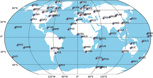
The monitoring network is shown in Figure 2, where data streams of all the stations are available in real-time via the internet from IGS Real-Time Service (RTS) caster. We intentionally select the monitoring stations that are not involved in the precise clock estimation. However, in Africa, South America and some marine areas, some overlapping stations are included for the quality monitoring as there are almost no redundant real-time stations available.

Figure 2. Monitoring station network with 70 globally distributed real-time stations.

Some details about the data and network, as well as the parameters of the observation model and data processing strategies used in our experiments are summarized in Table 2.

Table 2. Data and processing parameters used in the experimental evaluation.

Items	Description
Date	Day of Year (DOY): 204–225, 2021
Tracking data	70 globally distributed real-time stations
Observation	Ionosphere-free code and carrier phase combination
Positioning mode	Fix station coordinates to IGS weekly solution
Satellite system	GPS
Satellite product	GFZ real-time satellite products from caster: products.igs-ip.net:2101 with mountpoint SSRA00GFZ0
Sampling rate	1 s
Receiver clock bias	Estimated as white noise for every epoch
ZTD	Saastamoinen model correction and estimated as random-walk process
Mapping function	Global Mapping Function (GMF)
Carrier phase ambiguity	Estimated as a constant for an observation arc
Station/satellite phase center	igs14.atx
Phase wind-up	Corrected
Relativity effect	IERS conventions 2010
Station displacement	IERS conventions 2010

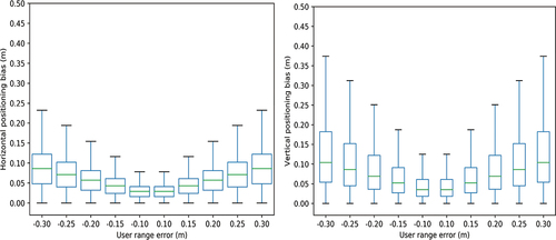
In order to determine the threshold $\delta$ beyond which an alarm should be triggered, the impacts of different user range errors caused by product biases on the positioning are investigated for each satellite at each station by adding a simulated error to the observed minus computed measurement $\mathrm{\nabla }l$, and the expression is shown below:

(20) $\begin{array}{rl}& \mathrm{\nabla }{x}_k^i={\left(A_k^T{P}_{kk}{A}_k+{\tilde{P}}_{x_k}\right)}^{-1}{A}_k^T{P}_{kk}\cdot \mathrm{\nabla }{l}_k^i,\\ & k=1,\dots ,n;i=1,\dots ,m\end{array}$(20)

Where $\mathrm{\nabla }{l}_k^i$ is the measurement vector with all members zero except for the members corresponding to the i-th satellite which is set to be the simulated error, i.e. the value in the horizontal axis of Figure 3, $\mathrm{\nabla }{x}_k^i$ is the positioning bias caused by the product bias of satellite $i$, the subscript, superscript and other symbols have the same meaning with Equation (6)(6) $\left[\begin{array}{c}{v}_1\\ v_2\\ \begin{array}{c}⋮\\ v_n\end{array}\end{array}\right]=\left[\begin{array}{cc}{A}_1& \begin{array}{cc}& \end{array}0\\ & A_2& \begin{array}{cc}& \end{array}\\ \begin{array}{c}\\ 0\end{array}& \begin{array}{c}\\ \end{array}& \begin{array}{c}\begin{array}{cc}\ddots & \end{array}\\ \begin{array}{cc}& A_n\end{array}\end{array}\end{array}\right]\cdot \left[\begin{array}{c}{\hat{x}}_1\\ {\hat{x}}_2\\ \begin{array}{c}⋮\\ {\hat{x}}_n\end{array}\end{array}\right]+\left[\begin{array}{c}{C}_1^i\\ C_2^i\\ \begin{array}{c}⋮\\ C_n^i\end{array}\end{array}\right]\cdot \left[{\hat{b}}^i\right]-\left[\begin{array}{c}{l}_1\\ l_2\\ \begin{array}{c}⋮\\ l_n\end{array}\end{array}\right],P=\left[\begin{array}{cc}{P}_{11}& \begin{array}{cc}& \end{array}0\\ & P_{22}& \begin{array}{cc}& \end{array}\\ \begin{array}{c}\\ 0\end{array}& \begin{array}{c}\\ \end{array}& \begin{array}{c}\begin{array}{cc}\ddots & \end{array}\\ \begin{array}{cc}& P_{nn}\end{array}\end{array}\end{array}\right]$(6) and (7(7) $\left[\begin{array}{cc}\begin{array}{ccc}{A}_1^T{P}_{11}{A}_1+{\tilde{P}}_{x_1}& 0& 0\\ & \ddots & 0\\ & A_n^T{P}_{nn}{A}_n+{\tilde{P}}_{x_n}\end{array}& \begin{array}{c}{A}_1^T{P}_{11}{C}_1\\ ⋮\\ A_n^T{P}_{nn}{C}_n\end{array}\\ \begin{array}{cc}sym& \end{array}& \sum _{k=1}^{n}C{{ }_k^i}^T{P}_{kk}{C}_k^i\end{array}\right]\cdot \left[\begin{array}{c}{\hat{x}}_1\\ ⋮\\ \begin{array}{c}{\hat{x}}_n\\ {\hat{b}}^i\end{array}\end{array}\right]=\left[\begin{array}{c}{A}_1^T{P}_{11}{l}_1\\ ⋮\\ \begin{array}{c}{A}_n^T{P}_{nn}{l}_n\\ \sum _{k=1}^{n}C{{ }_k^i}^T{P}_{kk}{l}_k\end{array}\end{array}\right]$(7) ). The statistical results in Figure 3 show that the positioning bias increases with the magnitude of the user range errors. When the magnitude of the user range error reaches 0.2 m, the median values of both the horizontal and vertical positioning biases are larger than 0.05 m and the maximum values are about 0.15 and 0.25 m, respectively. When the magnitude of the product bias is 0.15 m, most of the horizontal and vertical positioning biases are within 0.10 and 0.15 m, respectively. Considering the impacts of the different product biases and the sensitivity of the quality monitoring method, $\delta$ is set to be 0.2 m, which means a satellite product is seen as normal when the its product bias is less than 0.2 m.

Figure 3. Statistical analysis of the impacts of different user range errors caused by product biases on the positioning results in the horizontal (left) and vertical directions (right).

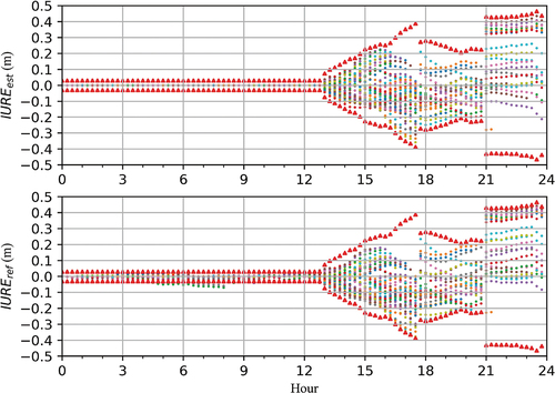
Before discussing the statistic results of the quality monitoring system, we take a look at an example of $IUR{E}_{est}$ and $IUR{E}_{ref}$ values as well as the corresponding quality indicators shown in Figure 4. When the satellite product can pass the detection of PPP QC for at least 70% of its tracking stations, the product bias of this satellite will not be estimated and their values are all zeros. Therefore, the quality indicator of this satellite is set to be 0.03 m according to Equation (14)(14) $\begin{array}{c}Q{I}^i=\underset{j\in S^i}{max}\left(\left|IUR{E_{est}}_j^i\right|\right)+0.03\end{array}$(14) . From Figure 4 we can find that before about 13:00 UTC the satellite product biases of G15 are not estimated and their $IUR{E}_{est}$ values are all zeros and the corresponding quality indicators are 0.03 m. Meanwhile, the $IUR{E}_{ref}$ values are smaller than 0.1 m, which means the satellite product is normal. After 13:00 UTC, the $IUR{E}_{ref}$ values of different stations get larger, which means the satellite products are biased. Meanwhile, the $IUR{E}_{est}$ values of different stations get larger and are close to the $IUR{E}_{ref}$, which means the product bias estimation is correct. In addition, the quality indicators based on the $IUR{E}_{est}$ can cover all the $IUR{E}_{ref}$ values when the satellite products are biased and thus the alarms can be triggered effectively.

Figure 4. An example of $IUR{E}_{est}$ (top) and $IUR{E}_{ref}$ (bottom) for G15, the red triangles represent the positive and negative quality indicators. The dots represent the $IUR{E}_{est}$ in the top plot and $IUR{E}_{ref}$ in the bottom plot, different colors represent different stations.

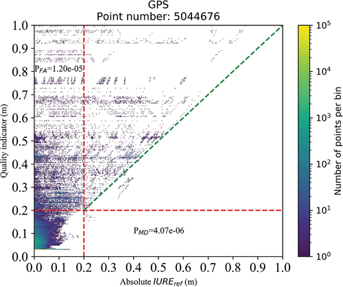
Figure 5 shows the 20-day quality monitoring results. One point corresponds to one GPS observation, whose abscissa value represents its absolute $IUR{E}_{ref}$ value and the ordinate value represents the quality indicator generated by the quality monitoring system. About 98.5% points located in the square area in the lower left corner, which means that both the satellite products and the monitoring results are normal. The points located in the square area in the upper right corner mean that the satellite products are biased and the alarms are triggered. In addition, because the quality indicators are larger than or equal to the absolute $IUR{E}_{ref}$ values, the points mainly locate in the upper triangle area. The points located in the rectangular area in the lower right corner mean that the satellite products are biased but no alarms are triggered. These points are classified as missed detections and the missed detection rate is $4\times {10}^{-6}$ for this experiment. The points located in the rectangular in upper left corner are not all false alarms, which depends on whether the $\underset{j\in S^i}{max}\left(\left|IUR{E_{ref}}_j^i\right|\right)$ is larger than the threshold $\delta$ or not. If the $\underset{j\in S^i}{max}\left(\left|IUR{E_{ref}}_j^i\right|\right)$ is larger than the $\delta$, these points are classified as correct alarms according to the definition in Table 1. Otherwise, these points are classified as false alarms and the false alarm rate is $1.2\times {10}^{-5}$ for this experiment. Furthermore, about 91.7% of satellite products can pass the detection of PPP QC for at least 70% of their tracking stations and the ordinate values of the corresponding points are 0.03 m.

Figure 5. Bivariate histogram showing the absolute $IUR{E}_{ref}$ compared to the corresponding quality indicators for GPS satellites from DOY 204 to 225, 2021.

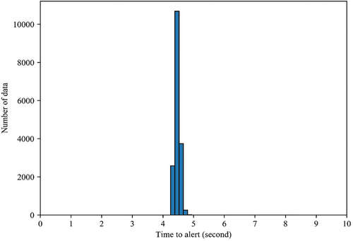
The TTA of the quality monitoring system is shown in Figure 6. The TTA is defined as the time elapsed from a quality event occurring to the alarm received by the users. It consists of three parts: 1) observation data and satellite products collection, 2) PPP data processing and product bias estimation, 3) uploading the quality information and sending to users. The three parts can run in parallel and the TTA values are mainly within 5 s and the mean value is 4.47 s as shown in Figure 6.

Figure 6. Histogram of the distribution of time to alarm (TTA).

4. An example of successful detection

For better understanding of the algorithm of the proposed method, we picked up a typical identified event for detailed investigation, for which large biases occur for both orbit and clock products.

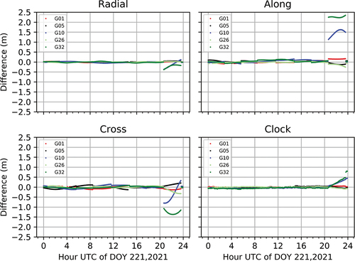
In the product comparison, since the most radial biases can be assimilated by the clock biases (Lou et al. 2014; Montenbruck, Steigenberger, and Hauschild 2015), the radial biases should be eliminated from the clocks before comparison. It should be noted that the good clock products should be stable over the time and the systematic bias can be assimilated by the carrier-phase ambiguity and thus hardly affect the positioning. From the product comparison result, G10 and G32 contain large biases, the differences are shown in Figure 7 with other three satellites with good agreement as example. The orbits of G10 and G32 have large jumps at 20:40 Coordinated Universal Time (UTC). From 20:40 to 23:40 UTC, the biases for the orbit of G10 range from −0.37 to 0.1 m, 1.1 to 1.6 m and −0.8 to 0.3 m for the radial, along and cross directions, respectively, and the clock bias has become a linear drift since 20:40 UTC and reaches to 0.47 m at 23:40 UTC. From 20:40 to 23:40 UTC, the biases for the orbit of G32 range from −0.38 to −0.18 m, 2.2 to 2.3 m and −1.3 to 1.1 m for the radial, along and cross directions, respectively, and the clock bias has become a linear drift since 20:40 UTC and reaches to 0.49 m at 23:35 UTC. After 23:40 UTC, the orbit biases of G10 and G32 become normal and are smaller than 5 cm, 10 and 10 cm for the radial, along and cross directions, respectively, the clock bias of G10 keeps stable with value of 0.47 m, while the clock bias of G32 has a jump at 23:40 UTC and reaches to 0.81 m.

Figure 7. Difference between the real-time satellite product and GBM final product on DOY 221, 2021, in the radial (top-left), along (top-right) and cross (bottom-left) directions, and that of clock offset (bottom-right) after eliminating orbit radial differences. Satellite G10 and G32 have large differences, whereas the others with good agreement are selected for comparison.

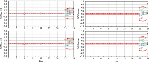
The quality monitoring procedure has detected the abnormal of products of G10 and G32 and the estimated satellite product biases are shown in Figure 8. The estimated radial biases for G10 have become larger since 20:37 UTC and reach 0.48 m at 23:40 UTC and then keep stable. The estimated along and cross biases for G10 have opposite large jumps with value of about 1 m at 20:37 UTC, and from 20:37 to 23:40 UTC the values of along and cross biases range from 1.08 to 1.75 m and from −1.01 to 0.24 m, respectively, and after 23:40 UTC the along and cross biases both become normal and are smaller than 10 cm. The estimated radial biases for G32 have become larger since 20:36 UTC and reach to 0.51 m at 23:35 and afterward increase to 0.90 m and keep stable. In addition, the estimated along and cross biases for G32 have opposite large jumps with values of about 2.2 and 1.09 m at 20:37 UTC, and afterward the biases range between 2.0 and 2.5 m for the along component and between −1.0 and −1.5 m for the cross component. The $IUR{E}_{est}$ generated using the estimated product biases are shown in the top part of Figure 9. The red triangles represent the positive and negative quality indicators calculated using Equation (14)(14) $\begin{array}{c}Q{I}^i=\underset{j\in S^i}{max}\left(\left|IUR{E_{est}}_j^i\right|\right)+0.03\end{array}$(14) . We can find that the quality indicators can cover all the $IUR{E}_{ref}$ value in the bottom part of Figure 9, which means that when the $IUR{E}_{ref}$ exceeds the $\delta$, an alarm can be triggered instantly.

Figure 8. Estimated satellite product errors of G10 (left) and G32 (right). The red dots represent that an alarm is issued.

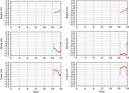
Figure 9. $IUR{E}_{est}$ and $IUR{E}_{ref}$ values for G10 (left) and G32 (right), the red triangles represent the positive and negative quality indicators. The dots represent the $IUR{E}_{est}$ in the top plot and $IUR{E}_{ref}$ in the bottom plot, different colors represent different stations.

5. PPP validation

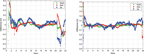
We further use PPP and some IGS reference stations to validate the contribution of the quality monitoring for the case shown in Section 4 by comparing the positioning performances of PPP solutions with and without the detected problematic satellites. The raw kinematic PPP results using GPS observations for station OUS2 and MAC1 are shown in Figure 10. We can see that the positioning results have become worse since 20:37 UTC. The maximum errors for the horizontal and vertical directions reach up to 0.26 m and 0.41 m, respectively. Such large positioning errors are not allowed for high accuracy applications.

Figure 10. Raw kinematic PPP results using GPS observations and GFZ real-time satellite products for station OUS2 (left) and WHIT (right) on DOY 221, 2021.

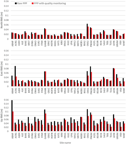
The kinematic results in Figure 11 represent that with the quality monitoring the large positioning errors caused by the biased satellite product are corrected to some extent. However, the positioning errors are still not good enough because the exclusion of observations from problematic satellites also causes the decrease of the observation number and leads to a poor satellite geometry. The statistic values in Figure 12 show that with the quality monitoring the RMS values in the north, east and up directions for 35 stations can be reduced from 2.5, 4.0 and 6.2 cm to 2.2, 3.2 and 4.5 cm with an improvement of 12%, 10% and 27%, respectively.

Figure 11. Kinematic PPP results using GPS observations and GFZ real-time satellite products for station OUS2 (left) and WHIT (right) with and without the quality monitoring on DOY 221, 2021. Black points are the raw results and red points are the results excluding the detected problematic satellites.

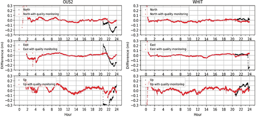
Figure 12. RMS of the difference between kinematic PPP results and the reference coordinates in the north (N), east (E) and up (U) directions for the entire day at 35 stations.

6. Conclusions

The RTPPS is recognized as the most promising system by providing various products including real-time precise orbits and clocks, UPD and regional augmentation information for users to achieving centimeter-level positioning with a stand-alone receiver in real-time. However, the unexpected biases in the real-time satellite orbit and clock products limit its practicability, especially for safety- and liability-critical applications. In this study, we propose a new method for quality monitoring of the real-time orbit and clock products in the state domain using a monitoring station network. The possible problematic satellites are first detected based on the results of PPP QC among their tracking stations. The product biases of these problematic satellites are represented by clock bias and orbital biases in the radial, along and cross directions, where the clock bias can be assimilated by the radial component for better estimability since they are highly correlated with each other. These parameters are estimated in the monitoring station network using the extended PPP model and the quality indicators can be calculated based on the estimated product biases. An alarm can be triggered when the quality indicator is larger than a pre-defined threshold. An iterative data processing procedure is employed to detect and identify any potentially problematic satellite until no satellite is voted out based on the observation residuals.

According to the 20-day experiment, the quality monitoring method can detect most problematic satellites effectively with missed detection rate $4\times {10}^{-6}$ and false alarm rate $1.2\times {10}^{-5}$ and the mean TTA is 4.47 s. A typical identified event is presented, where two satellites have large biases in both orbit and clock products. The product biases are investigated carefully by comparing the real-time product and GBM final product. The estimated product biases have a good agreement with the comparison results of the real-time and final product and the alarms are issued instantly when the quality indicators are larger than $0.2\mathrm{m}$. With the quality monitoring, the observations from the problematic satellite can be excluded in PPP data processing at the user-level. The PPP results in terms of RMS of position differences with respect to the ground true for 35 stations in the north, east and up directions can be reduced from 2.5, 4.0 and 6.2 cm to 2.2, 3.2 and 4.5 cm with an improvement of 12%, 10% and 27%, respectively.

Disclosure statement

No potential conflict of interest was reported by the author(s).

Data availability statement

The real-time satellite orbit and clock products used in this study are available from caster: products.igs-ip.net:2101 with mountpoint SSRA00GFZ0.

Additional information

Funding

This work is funded by the National Natural Science Foundation of China (42030109).

Notes on contributors

Run Ji

Run Ji is a Ph.D. candidate at German Research Centre for Geosciences (GFZ) and Technical University of Berlin. His current research focuses on real-time precise point positioning and multi-sensor fusion.

Xinyuan Jiang

Xinyuan Jiang is currently working toward the Ph.D. degree at Technical University of Berlin and working as a researcher at the German Research Centre for Geosciences (GFZ). His current research mainly involves real-time precise positioning services and its software development.

Xinghan Chen

Xinghan Chen is currently working at German Research Center for Geosciences (GFZ), Potsdam, Germany. His major research interests contain GNSS precise orbit determination, positioning, and GNSS applications.

Huizhong Zhu

Huizhong Zhu is a professor of Liaoning Technical University, China, and head of the School of Geomatics. His research activities focus on precise applications of GNSS such as RTK, PPP, real-time PPP, precise orbit determination.

Maorong Ge

Maorong Ge received his Ph.D. at the Wuhan University. He is now a senior scientist at GFZ, Potsdam, Germany. He has been in charge of the IGS Analysis Center at GFZ and is now leading the real-time software group. His research interests are GNSS data processing and related algorithms and software development.

Frank Neitzel

Frank Neitzel is professor of Geodesy and Adjustment Theory and managing director of the Institute of Geodesy and Geoinformation Science at Technische Universität Berlin, Germany. His current research focuses on rigorous solutions of nonlinear adjustment problems, filter methods, deformation monitoring, and measurement and model-based structural analysis.

References

- Baarda, W. 1968. “A Testing Procedure for Use in Geodetic Networks.” Netherland Geodetic Commission 2 (5): 53–65.
- Blewitt, G., C. Kreemer, W. Hammond, H. Plag, S. Stein, and E. Okal. 2006. “Rapid Determination of Earthquake Magnitude Using GPS for Tsunami Warning Systems.” Geophysical Research Letters 33 (11). doi:10.1029/2006GL026145.
- Cheng, C., Y. Zhao, L. Li, J. Cheng, and X. Sun. 2018. “Preliminary Analysis of URA Characterization for GPS Real-time Precise Orbit and Clock Products”. In 2018 IEEE/ION Position, Location and Navigation Symposium (PLANS), 615–621. IEEE. doi:10.1109/PLANS.2018.8373434.
- Collins, P., S. Bisnath, F. Lahaye, and P. Héroux. 2010. “Undifferenced GPS Ambiguity Resolution Using the Decoupled Clock Model and Ambiguity Datum Fixing.” NAVIGATION, Journal of the Institute of Navigation 57 (2): 123–135. doi:10.1002/j.2161-4296.2010.tb01772.x.
- Defraigne, P., Q. Baire, and N. Guyennon. 2007. “GLONASS and GPS PPP for Time and Frequency Transfer”. In 2007 IEEE International Frequency Control Symposium Joint with the 21st European Frequency and Time Forum, 909–913. IEEE. doi:10.1109/FREQ.2007.4319211.
- Deng, Z., M. Fritsche, M. Uhlemann, J. Wickert, and H. Schuh. 2016. “Reprocessing of GFZ multi-GNSS Product GBM”. In IGS Workshop, 8–12. http://acc.igs.org/workshop2016/presentations/Plenary_01_06.pdf
- Du, Y., J. Wang, C. Rizos, and A. El-Mowafy. 2021. “Vulnerabilities and Integrity of Precise Point Positioning for Intelligent Transport Systems: Overview and Analysis.” Satellite Navigation 2 (1): 1–22. doi:10.1186/s43020-020-00034-8.
- Duan, B., U. Hugentobler, J. Chen, I. Selmke, and J. Wang. 2019. “Prediction versus Real-time Orbit Determination for GNSS Satellites.” GPS Solutions 23 (2): 1–10. doi:10.1007/s10291-019-0834-2.
- Fu, W., G. Huang, Q. Zhang, S. Gu, M. Ge, and H. Schuh. 2019. “Multi-GNSS Real-time Clock Estimation Using Sequential Least Square Adjustment with Online Quality Control.” Journal of Geodesy 93 (7): 963–976. doi:10.1007/s00190-018-1218-z.
- Ge, M., J. Douša, X. Li, M. Ramatschi, T. Nischan, and J. Wickert. 2012. “A Novel Real-time Precise Positioning Service System: Global Precise Point Positioning with Regional Augmentation.” Journal of Global Positioning Systems 11 (1): 2–10. doi:10.5081/jgps.11.1.2.
- Ge, M., G. Gendt, M.A. Rothacher, C. Shi, and J. Liu. 2008. “Resolution of GPS Carrier-phase Ambiguities in Precise Point Positioning (PPP) with Daily Observations.” Journal of Geodesy 82 (7): 389–399. doi:10.1007/s00190-007-0187-4.
- Heng, L., G. Gao, T. Walter, and P. Enge. 2011. “Statistical Characterization of GPS Signal-in-space Errors.” In Proceedings of the 2011 international technical meeting of the Institute of Navigation, 312–319. https://www.ion.org/publications/abstract.cfm?articleID=9472
- Hexagon. 2021. “Global Breakthrough in PPP Technology: RTK from the Sky”. Available from https://bit.ly/35M8yDM
- Kazmierski, K., R. Zajdel, and K. Sośnica. 2020. “Evolution of Orbit and Clock Quality for Real-time multi-GNSS Solutions.” GPS Solutions 24 (4): 1–12. doi:10.1007/s10291-020-01026-6.
- Laurichesse, D., L. Cerri, J.P. Berthias, and F. Mercier. 2013. “Real Time Precise GPS Constellation and Clocks Estimation by Means of a Kalman Filter.” In Proceedings of the 26th international technical meeting of the satellite division of the institute of navigation (ION GNSS+ 2013), 1155–1163. https://www.ion.org/publications/abstract.cfm?articleID=11318
- Laurichesse, D., F. Mercier, J.P. BERTHIAS, P. Broca, and L. Cerri. 2009. “Integer Ambiguity Resolution on Undifferenced GPS Phase Measurements and Its Application to PPP and Satellite Precise Orbit Determination.” Navigation 56 (2): 135–149. doi:10.1002/j.2161-4296.2009.tb01750.x.
- Li, X., X. Chen, M. Ge, and H. Schuh. 2019. “Improving multi-GNSS Ultra-rapid Orbit Determination for Real-time Precise Point Positioning.” Journal of Geodesy 93 (1): 45–64. doi:10.1007/s00190-018-1138-y.
- Li, Z., W. Chen, R. Ruan, and X. Liu. 2020. “Evaluation of PPP-RTK Based on BDS-3/BDS-2/GPS Observations: A Case Study in Europe.” GPS Solutions 24 (2): 1–12. doi:10.1007/s10291-019-0948-6.
- Li, X., M. Ge, H. Zhang, T. Nischan, and J. Wickert. 2013. “The GFZ Real-time GNSS Precise Positioning Service System and Its Adaption for COMPASS.” Advances in Space Research 51 (6): 1008–1018. doi:10.1016/j.asr.2012.06.025.
- Li, X., X. Zhang, and M. Ge. 2011. “Regional Reference Network Augmented Precise Point Positioning for Instantaneous Ambiguity Resolution.” Journal of Geodesy 85 (3): 151–158. doi:10.1007/s00190-010-0424-0.
- Liu, T., B. Zhang, Y. Yuan, and M. Li. 2018. “Real-Time Precise Point Positioning (RTPPP) with Raw Observations and Its Application in Real-time Regional Ionospheric VTEC Modeling.” Journal of Geodesy 92 (11): 1267–1283. doi:10.1007/s00190-018-1118-2.
- Lou, Y., W. Zhang, C. Wang, X. Yao, C. Shi, and J. Liu. 2014. “The Impact of Orbital Errors on the Estimation of Satellite Clock Errors and PPP.” Advances in Space Research 54 (8): 1571–1580. doi:10.1016/j.asr.2014.06.012.
- Montenbruck, O., P. Steigenberger, and A. Hauschild. 2015. “Broadcast versus Precise Ephemerides: A multi-GNSS Perspective.” GPS Solutions 19 (2): 321–333. doi:10.1007/s10291-014-0390-8.
- Petit, G., and B. Luzum. 2010. IERS Conventions 2010, 179. IERS Technical Note, 36. Frankfurt am Main, Germany: Verlag des Bundesamts für Kartographie und Geodäsie.
- Rodriguez-Solano, C., M. Brandl, X. Chen, M. Herwig, A. Kipka, P. Kreikenbohm, H. Landau, et al., 2019. “Integrity Real-time Performance of the Trimble RTX Correction Service.” In Proceedings of the 32nd International Technical Meeting of the Satellite Division of The Institute of Navigation (ION GNSS+ 2019), 485–507. doi:10.33012/2019.16863.
- Teunissen, P.J.G.2000.Testing Theory.Delft: Delft University Press. An Introduction
- Wang, Y., and J. Shen. 2020. “Real-time Integrity Monitoring for a Wide Area Precise Positioning System.” Satellite Navigation 1 (1): 1–10. doi:10.1186/s43020-020-00018-8.
- Weber, G., L. Mervart, Z. Lukes, C. Rocken, and J. Dousa. 2007. “Real-time Clock and Orbit Corrections for Improved Point Positioning via NTRIP.” In Proceedings of the 20th international technical meeting of the satellite division of the institute of navigation (ION GNSS 2007), 1992–1998. https://www.ion.org/publications/abstract.cfm?articleID=7413
- Weinbach, U., M. Brandl, X. Chen, H. Landau, F. Pastor, N. Reussner, and C. Rodriguez-Solano. 2018. “Integrity of the Trimble® CenterPoint RTX Correction Service.” Proceedings of the 31st International Technical Meeting of The Satellite Division of the Institute of Navigation (ION GNSS+ 2018). doi:10.33012/2018.15971.
- Wu, J., S. Wu, G. Hajj, W. Bertiger, and S. Lichten. 1993. “Effects of Antenna Orientation on GPS Carrier Phase.” Astrodynamics 1991: 1647–1660.
- Yang, L., J. Wang, N.L. Knight, and Y. Shen. 2013. “Outlier Separability Analysis with a Multiple Alternative Hypotheses Test.” Journal of Geodesy 87 (6): 591–604. doi:10.1007/s00190-013-0629-0.
- Yang, Y., and J. Xu. 2016. “GNSS Receiver Autonomous Integrity Monitoring (RAIM) Algorithm Based on Robust Estimation.” Geodesy and Geodynamics 7 (2): 117–123. doi:10.1016/j.geog.2016.04.004.
- Zumberge, J.F., M.B. Heflin, D.C. Jefferson, M.M. Watkins, and F.H. Webb. 1997. “Precise Point Positioning for the Efficient and Robust Analysis of GPS Data from Large Networks.” Journal of Geophysical Research: Solid Earth 102 (B3): 5005–5017. doi:10.1029/96JB03860.
- Zuo, X., X. Jiang, P. Li, J. Wang, M. Ge, and H. Schuh. 2021. “Square Root Information Filter for multi-GNSS Real-time Precise Clock Estimation.” Satellite Navigation 2 (1): 1–14. doi:10.1186/s43020-021-00060-0.