“Hot street” of crime detection in London borough and lockdown impacts

ABSTRACT

In recent years, the police intervention strategy “Hot spots policing” has been effective in combating crimes. However, as cities are under the intense pressure of increasing crime and scarce police resources, police patrols are expected to target more accurately at finer geographic units rather than ballpark “hot spot” areas. This study aims to develop an algorithm using geographic information to detect crime patterns at street level, the so-called “hot street”, to further assist the Criminal Investigation Department (CID) in capturing crime change and transitive moments efficiently. The algorithm applies Kernel Density Estimation (KDE) technique onto street networks, rather than traditional areal units, in one case study borough in London; it then maps the detected crime “hot streets” by crime type. It was found that the algorithm could successfully generate “hot street” maps for Law Enforcement Agencies (LEAs), enabling more effective allocation of police patrolling; and bear enough resilience itself for the Strategic Crime Analysis (SCA) team’s sustainable utilization, by either updating the inputs with latest data or modifying the model parameters (i.e. the kernel function, and the range of spillover). Moreover, this study explores contextual characteristics of crime “hot streets” by applying various regression models, in recognition of the best fitted Geographically Weighted Regression (GWR) model, encompassing eight significant contextual factors with their varied effects on crimes at different streets. Having discussed the impact of lockdown on crime rates, it was apparent that the land-use driven mobility change during lockdown was a fundamental reason for changes in crime. Overall, these research findings have provided evidence and practical suggestions for crime prevention to local governors and policy practitioners, through more optimal urban planning (e.g. Low Traffic Neighborhoods), proactive policing (e.g. in the listed top 10 “Hot Streets” of crime), publicizing of laws and regulations, and installations of security infrastructures (e.g. CCTV cameras and traffic signals).

KEYWORDS:

• Hot street
• crime
• kernel density estimation
• spatial regression
• lockdown
• mobility change

1. Introduction

Crime has long been a social security issue of public concern. It does not occur randomly or evenly in the geographical environment, instead is inevitably related to local population, environment, and society context, with manifestation in a certain temporal and spatial pattern. Hence, a timely grasp of the distribution of crime and the trajectory of criminals could contribute to crime prevention and control. In recent years, the development of the Geographic Information System (GIS) and crime mapping techniques has gradually improved the public’s ability to understand and identify crimes, thus enabling Law Enforcement Agencies (LEAs) to carry out more effective crime reduction measures. Poulsen and Birchall (2002) claimed that GIS assisted analysts in investigating crime trends, highlighted areas for police patrolling, provided the government with crime deterrent evidence, and afforded the public better understanding of local crime situations. Amongst the literature of crime analysis methods, Hot Spots Analysis had been widely applied in real-life scenarios, such as the “Hot Spots Policing” strategy targeting the patrolling “hot spots” areas with more than average crime occurrences or unusually higher risks of victimization. By default, a “hot spot” is considered as a unit of area; but, in fact, crime hot spots could also be viewed in the form of points or lines (Harries 1999), representing places or street segments. To concentrate criminal investigations in recognized “hot” locations could hereafter provide higher accuracy. However, recognizing “hot spots” alone does not lead to effective utilization of the police resources for granted, considering the inconsistent observation duration and the effect lag. In light of these, crime pattern analysis down to street level would be more informative and accurate, since the street pattern was the main feature of criminals’ search behavior (Brantingham, and Brantingham 2010). In reality, various commercial buildings are normally located along a road between home and workplaces, where the large flow of people and numerous physical elements provide shelters for potential offenders, and create a lot of criminal opportunities. For example, Lowman, Rengert, and Wasilchick (1987)’s study on burglary in Delaware County found that the crime scene was significantly associated with the primary commuting route. Weisburd and Green (1995) suggested that a series of drug dealing activities and drug dens could be found along the streets with significant patterns, due to drug dealers’ preference on trading in hidden locations along the streets, which rendered academia’s focus on recognizing drug “hot spots” along street segments. Rosser et al. (2017) had justified the better performance of street network-based methods for property crimes prediction comparing to grid-based alternatives.

This study attempts to develop a street-based algorithm detecting the crime “hot streets” by type in Haringey Borough of London in 2020, and to further compare the changes with that of 2019. To begin with, the study introduces an improved spatial autocorrelation, namely network autocorrelation, to test whether crime incidents alongside street network are Complete Spatial Randomness (CSR) distribution, by adapting the research object and corresponding weights to street segments; it is taken as the premise for discussion on crime spillovers by rejecting the CSR. Secondly, Kernel Density Estimation (KDE) is integrated into the “hot street” detection algorithm to measure the influence from neighbors on a one-dimensional network, rather than on a conventional two-dimensional plane. Finally, GIS is adopted to map crimes against the street network and the crime “hot streets”, in expectation to facilitate strategies on police patrolling frequency as well as to reminder residents with alerting messages when appropriate. This study has involved six major crime types: property crimes, anti-social behavior, violence and sexual offenses, public order offenses, drug crimes, and possession of weapons. Besides, eight contextual features relating to crime “hot streets” are discussed, namely carriageway width, street length, the Index of Multiple Deprivation (IMD), average house price, average household income, mobility change, number of CCTV (closed-circuit television) cameras, and number of traffic signals. To investigate their relations to crime, Spatial Econometrics (SEs) models and the Geographically Weighted Regression (GWR) model are utilized in a comparative manner. In general, this project tries to explain the mechanism of crime-influential effects from aforementioned features at the case study borough, with a focus on discussing the lockdown impacts on crime change regarding to land use driven mobility change.

Following the introduction of the research motivation, aims and methods adopted above, Section 2 illustrated the background of the project by correlating it with the existing literature in the field; and Section 3 introduced the crime scenarios in the study area, data sources and methodologies, followed by results’ presentation and analyses in Section 6. Section 5 recognized the research limitations and Section 6 outlined the conclusions and future work.

2. Background and literature

Empirical studies have shown that the occurrence of criminal activities is not random. Crime Pattern Theory (Brantingham, and Brantingham 1984) suggests that crime only occurs when the victim’s trajectory or the location of the target object overlaps with the criminal’s activity area. The likelihood of crime occurring in a specific space-time is determined by convergence of potential offenders, appropriate targets, and the absence of effective guardianship (Cohen, and Felson 1979), which reveals the importance of environment in inducing crimes. The case study from La Vigne (1996) on crime prevention in the Washington Metro indicated that the supervision of station attendants is the sole crucial means of predicting an assault, whereas CCTV cameras could exert psychological pressure on potential criminals. As stated in the Geometry of Crime (Brantingham, and Brantingham 2016), people carry out daily activities in an environment where society, economy, and politics integrate, such as homes, office buildings, schools, and shopping malls, and regular pathways that connect these places. Such repeated trips on weekdays and weekends have gradually formed routine activity patterns for the majority, but also been followed by potential criminals looking for crime opportunities in their familiar awareness space.

Some in-depth criminological studies have found the non-uniform distribution of crimes in geographical space. For instance, the longitudinal study of crimes in Seattle from 1989 to 2002 (Weisburd et al. 2004) found that 50% of the cases occurred on only 4.5% of street segments. Weisburd and Mazerolle (2000) further conducted a survey with indication that 56 drug “hot spots” in Jersey City accounted for only 4.4% of the city’s area. Such crime distributions could refer to the Pareto principle (Eck, Clarke, and Guerette 2007) in that, the top 20% of crime “hot spots” are responsible for 80% of criminal cases in the target area. Most state-of-the-art crime detection methods involve analysis at the micro-level, hence play a crucial role in criminals arrests and the deployment of policing resources. Among such methods, hot spots analysis has been commonly utilized, but mostly be mapped at areal geographic unit. O’Brien (2018) raised that there were zero-crime and low-crime streets within identified crime “hot spots”, whilst streets with high crime rates falling in crime cold spots, resulting in the negligence of potential severe crimes. Therefore, it is worthwhile to address the analytical scale issue relating to the accuracy of crime detection. Besides of the areal “hot spots”, Eck et al. (2005) discussed “repeat places hot spots” and “repeat streets hot spots” when mapping crimes, in the form of dots and lines respectively. For instance, earlier explorations in criminology were mainly based on individual crime cases in the form of dots but rendered the neglections of criminal aggregation and corresponding social factors (Reiss, and Farrington 1991), leading to the recommendation on performing crime pattern analysis on street level. Empirical studies have proved that using street segment as the study unit in criminology is more stable than reviewing broader “hot spots” (Weisburd et al. 2004; Weisburd, Groff, and Yang 2013; Taylor, Gottfredson, and Brower 1984; Andresen, and Malleson 2010). Taylor (1997) put forward a persuasive argument that, using street segment as a unit of analysis that conforms to ecological theories can better explain the crime mechanism. The rationale is that local land use can form the social and physical environment in and along the street segments, thereby shifting human beings’ behavior patterns. In general, a street segment is a unit larger than a place to compensate for addressing errors (Weisburd, and Green 1995), but smaller than an area to avoid ignoring some important characteristics hidden in clusters (Weisburd, Groff, and Yang 2013). Specifically, it has a high degree of openness, carries people’s daily activities, and inevitably brings about some safety issues. As suggested by crime pattern theory, those easily accessible paths provided by the street network have become active spaces for offenders (Brantingham, and Brantingham 1984), and their familiarities had made them into criminals looking for crime opportunities. Furthermore, streets on the fringe of the city could be high-risk streets (Angel 1968), since criminals may identify potential victim targets in the city center but stalk until a remote street to commit predatory crimes. In addition, the structure of streets also contributes to crime occurrence as pointed out by Brantingham and Brantingham (1993) that, grid streets are more likely to host crimes than cul-de-sacs and dead-end streets, since the former are conducive to offenders’ escape; also owing to the decrease in traffic volumes of the latter types of streets, crime risks may increase compounding with the decline in natural surveillance (Wagner 1997).

“Hot Street” has been formulated normally by calculating the number or the rate of certain events on a street segment. It is a commonly used method to identify streets with frequent accidents in real life (Mitra 2009; Xie, and Yan 2008; Hauer 1997), but bear with biases. Hauer et al. (2002) pointed out two shortcomings applying this approach to assess road safety as references for crime research: (1) if a small number of accidents occur over a long period, the calculation of annual average incidence becomes inaccurate, with a much larger standard deviation than the mean value; (2) considering the preconceived prejudice that prevails among the public, citizens tend to focus more on streets with either too many or few accidents, inducing to subject individual perception of road safety. To address aforementioned cons, Empirical Bayes had been suggested to tackle with the mean-deviation problem, but the method itself has higher requirements on analysts’ capability in decision making process against real-life problems (Hauer et al. 2002); GIS-featured methods then became more recommended and superior, with several empirical street-based crime geoprocessing methods: (1) Getis Ord Gi* statistics. Paisley (2017) adopted Gi* clustering algorithm to develop a map application on identifying crime trend alongside the streets in Los Angeles, and observing the environmental conditions around high crime streets; a GIS-based geographic model for spatio-temporal analysis of street crime in Atlanta, Georgia, Houston and Texas (Tom-Jack, Bernstein, and Loyola 2019) applied Getis Ord Gi* statistics to classify “hot streets” of crime based on the confidence levels; (2) KDE. Milić et al. (2020) conducted a case study in New Belgrade, Serbia, to identify traffic accident street hot spots, and concluded that the network based KDE is more accurate in detecting linear hot spots than the planar KDE, hence could further benefit crime hot street analysis; (3) A new technique “Hot Routes”. Tompson, Partridge, and Shepherd (2009) proposed a GIS-based method “Hot Routes”, which only relied on street names and grid references to calculate the crime rate per meter of London bus routes, presenting the crime risk distribution in the street view; (4) A search-window technique. Shiode and Shiode (2013) developed a network-based space-time search-window technique for street-level crime detection, and effectively identified space-time hotspots of drug dealings and assaults in Buffalo, New York.

The Getis-Ord G* statistics calculates the G* statistics for each element in the dataset, and judge whether it is statistically significant by its z-value and p-value. Those with high values and surrounded by other high values are statistically significant “hot spots”. In addition to Getis-Ord G* statistics, KDE, a completely different non-parametric method, had been also commonly used to detect crime clusters (Parzen 1962). KDE performs density calculations according to user-defined search bandwidth and kernel functions, to estimate the probability density function from the characteristics of the data sample itself, rather than assuming its distribution pattern based on prior knowledge (such as exponential or chi-square distributed). Moreover, KDE utilizes neighborhood information when evaluating the probability density of each sample point, which was thought to be helpful in improving the function discontinuity problem. Although G* statistics can measure the significance of a cluster at a certain confidence level, KDE provides greater flexibility in practice, allowing users to customize the search radius and the size of the output grid, to meet the requirements of reality. For example, the Strategic Crime Analysis (SCA) team can determine the search radius by evaluating the size of the police force or by assessing on the scale of different crime types, in reflection of KDE’s widely adoption in hot spots algorithms. Similarly, one research in India and Bangalore cities utilized the news feed data and KDE to recognize crime hot spots in the planar level (Prathap, and Ramesha 2020). Milić et al. (2020) put forward the network-based KDE and demonstrated its higher accuracy than the planar KDE when analyzing traffic accidents’ data. In hope of filling the gap applying KDE onto network level in crime research, this study will build up the algorithm on basis of network-based KDE to detect crime “hot streets” in the target area.

In 2020, the COVID-19 incurred lockdowns in UK had limited people’s movements. As suggested by Caminha et al. (2017) that since human mobility could be regarded as an agent of criminal activities, the lockdown related surge of floating population in some nations could promote excessively many property crimes in a super linear way. Cheung and Gunby (2021) explored the crime rate during the COVID-19 pandemic in New Zealand and stated that the change in mobility patterns upon lockdown policy had a significant impact on the crime rate. They demonstrated that the reduction in the population flow in grocery stores, pharmacies and nonresidential areas has a strong association with the decline in crime. In addition, the stay-at-home policy restricted people’s travel hence reduced the flow of people, followed by the sharp drop of crime incidents. This has even been described as the largest criminology experiment in history (Stickle, and Felson 2020). On the other hand, local land uses can be an indicator for human mobility, since the land use function serves human requirements, such as housing, working, entertainment and other events that impact essential travels (Lee, and Holme 2015); so, this study tried to use the land-use simulated mobility change index as the proxy to observe lockdown’s impact.

3. Data and methods

3.1. Crimes in study area

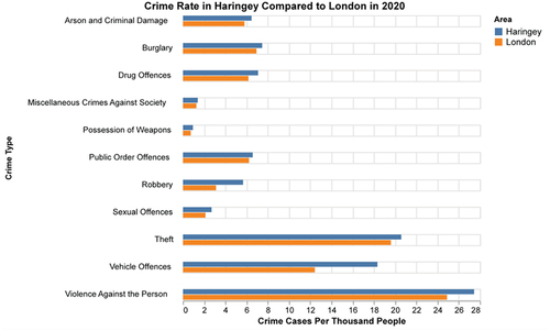
The study area, Haringey Borough of London, is a high-poverty borough in the north, straddling Inner London and Outer London, with a population of 275,900 and an area of 29.58 square kilometers. According to local government’s report, the BAME (Black, Asian and minority ethnic) group accounts for 38% of the local population, while other whites accounting for 26%. Haringey’s crime level is relatively high among London boroughs. For example, between October 2018 and September 2019, its domestic abuse crime rate was the third highest among all boroughs in London, with approximately 33 crimes per 10,000 people; and the knife crime rate ranked fourth at 6 per 10,000 people (https://www.met.police.uk/sd/stats-and-data/met/crime-data-dashboard/). In 2020, Haringey had about 105 crimes per 1000 people, which was almost 15% higher than the average in London (90 incidents per 1000 people). It could be seen from Figure 1 that, regardless of crime type, Haringey’s crime rate is higher than the average value in London; but the top three crime types, namely violence against the person, theft, and vehicle offenses, exhibited similar statistics with slight differences.

Figure 1. Crime rate in Haringey compared to London in 2020.

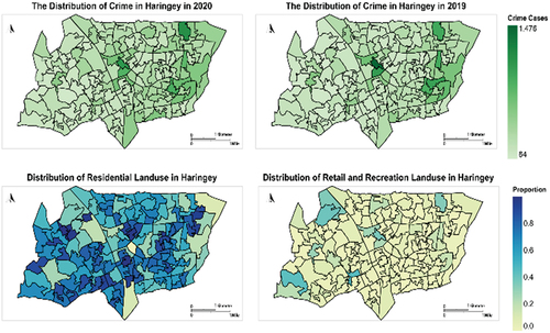
To further explore the crime incidents’ distribution in the borough (depicted in Figure 2), respective map on crimes in Haringey Borough of London in 2020 and 2019 had been drawn but with almost no change over time. It could be seen that the worst-hit area, Wood Green (located in the center of the borough), is a major commercial hub with more than 100 retail stores. In 2019, the number of crime cases in its corresponding Lower Layer Super Output Area (LSOA) reached at 1476, while other crime hot spots were scattered in the east of the borough. Comparatively, there were fewer crimes recorded in the western residential areas. It could be arrived at this stage that, there are more crimes in commercial areas, and less crimes in residential areas in the west and south of the borough. Stepping into 2020, some crime changes could be observed that, crimes overflowed from previous “hot spots” to their surrounding areas. This may be due to the COVID-19 pandemic related lockdown policy since 23 March 2020, when shops were asked to close and people’s travel was restricted, hence reducing the crime opportunities significantly.

Figure 2. Haringey’s crime distribution and land use distribution.

3.2. Data sources

3.2.1. Streetspace dataset

The street map had been derived from the work on London Streetspace Dataset shared by Nicolas Palominos from CASA UCL, including street attributes on name, code, classification, carriageway widths, and total widths. More detailed information could be obtained from the GitHub project (https://github.com/npalomin/streetspace_dataset_ldn).

3.2.2. Crime data

Referenced to report from Office for National Statistics (Flatley 2016), this study merged the 14 police recorded crimes into seven main types because that, property crime is taken as an illegal activity involving deprivation or destruction of property, which covers burglary, criminal damage and arson, vehicle crime, robbery, bicycle theft, theft from the person, shoplifting and other theft. The seven crime types of study are: 1) Anti-social behavior; 2) Drug crimes; 3) Violence and sexual offenses; 4) Property crimes: including Burglary, Criminal damage and arson, Vehicle crime, Robbery, Bicycle theft, Other theft, Shoplifting, Theft from the person; 5) Possession of weapons; 6) Public order offenses; and 7) Other crimes. Such data were collected from Met Police open data and local city council from 2017 to 2020.

3.2.3. Environment data

To identify the characteristics of “Hot Streets” of crime, environment data were collected from three aspects: road properties, the surrounding facilities, and the contextual background of the embracing LSOAs. Table 1 summarized the information and sources of the specific features, which are all objects with geospatial locations and other attributes, where the IMD is taken as the proxy for local poverty level, with higher value indicating for higher deprivation.

Table 1. Information of features.

Feature	Data Source
Street length, Carriageway width	Haringey street map
Park, Pub, Bus stop, CCTV cameras, Street lighting, Traffic signals, Zebra and pelican crossings [Note: These features refer to their counts.]	OpenStreetMap, the Haringey government
the Index of Multiple Deprivation (IMD), Average house price, Average household income, Mobility change	Ministry of Housing, London Datastore, GoogleCommunityReport,Open Street Map

3.3. Methods

3.3.1. “Hot street” algorithm design

The “Hot Street” algorithm was designed in the assumptions that: (1) crimes occur on the street, and (2) streets with crimes will not be affected by nearby crime-free streets; on the contrary, streets without crimes will be affected by neighboring streets with crimes. Kernel Gaussian function had been applied in the algorithm design as depicted in flowchart in Figure 3.

Figure 3. Flowchart of the crime hot street map.

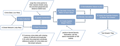
1. Ensure the assigned street network and cleaned crime data are in the same projected coordinate reference system.

2. Map crime incidents data in point format onto the corresponding nearest streets, using the shortest perpendicular distance.

3. Count the number of crimes on each street segment and divide it by the corresponding street’s length.

4. Set the search bandwidth at 100 meters, and use kernel function to calculate the weights of the shortest distance, between the center of each street segment and the centers of other street segments within the search bandwidth, to finally create a spatial weight matrix for each street (diagonal weights were set to 1).

5. The crime density calculations for streets are different. Set the default values of crime density of each street segment as 0.

• For crime street, the crime density is determined by itself and other crime streets within 100 meters, calculating in below formula:

(1) $D_c\left(S_i\right)={\sum }_{j=1}^n\mathit{K}\left(\frac{{\mathit{d}}_{\mathit{ij}}}{\mathit{h}}\right)\cdot C_j={\sum }_{j=1}^n\frac{1}{\sqrt{2\mathit{\pi }}}\mathit{exp}\left(-\frac{d_{ij}^2}{2h^2}\right)\cdot C_j$(1)

where D_c(S_i) is the crime density at crime street i (S_i), K is the weight of street j at distance d_ij to street i, h is the search bandwidth, C_j is crime per meter at street j, and n is the number of neighboring streets within h (including itself).

• For crime-free street, the crime density is determined by its neighboring crime streets within search bandwidth, the calculation is as below:

(2) $D_{\mathit{cf}}\left(S_a\right)={\sum }_{i=1}^m\frac{1}{\sqrt{2\mathit{\pi }}}\mathit{exp}\left(-\frac{d_{ai}^2}{2h^2}\right)\cdot D_c\left(S_i\right)$(2)

where D_cf (S_a) is the crime density at crime-free street a (S_a), d_ai is the distance between street a and street i, and m is the number of neighboring crime streets within h.

6) After calculating the crime densities of all streets, normalized all values by scaling them in the range of [0, 1]:

(3) $D_{\mathit{nor}}\left(S_t\right)=\frac{D\left(S_t\right)-D_{\mathit{min}}}{D_{\mathit{max}}-D_{\mathit{min}}}\mathit{\hspace{0.17em}}$(3)

where D_nor(S_t) and D(S_t) are the normalized and original crime densities of street t(S_t), respectively, D_min and D_max are the minimum value and maximum value of all crime densities.

7) Since the number of different crime types may vary greatly, setting a fixed value as the threshold of “Hot Street” may not be reliable. Hence, the quartile scheme is applied to generate the “Hot Street” map of crimes. Crime-free streets are not included but are classified as a separate category.

3.3.2. Network autocorrelation

Network Autocorrelation is spatial autocorrelation in nature, but refers to the correlation of a variable on itself according to the positions of different arcs observed in the network; to examine the events’ distribution on the arcs of a network, whether it is clustered, dispersed, or random, such as traffic accidents events (Black 2010). The mathematical equation and interpretation of the results are the same as spatial autocorrelation, but with different analyzing objects and spatial weights. This study utilized the most used spatial autocorrelation measure, Moran’s I, onto street level crime distribution detection, to gain insight into crime “hot streets” as follows.

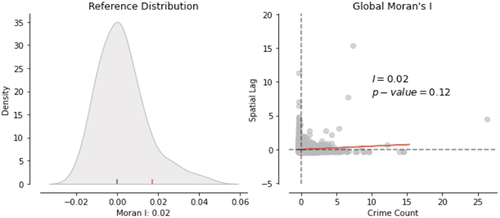
Under the null hypothesis of no existence of network autocorrelation, Global Moran’s I had been calculated as:

(4) $\mathit{I}=\frac{n}{{\sum }_i{\sum }_j{w}_{\mathit{ij}}}\frac{{\sum }_i{\sum }_j{w}_{\mathit{ij}}\left(x_i-\bar{x}\right)\left(x_j-\bar{x}\right)}{{\sum }_i{\left(x_i-\bar{x}\right)}^2},\mathit{i}\ne \mathit{j}\mathit{\hspace{0.17em}}$(4)

while Local Indicators of Spatial Association (LISA) had been calculated as:

(5) $I_i=\left(x_i-\bar{x}\right)\sum _i{w}_{\mathit{ij}}\left(x_j-\bar{x}\right),\mathit{i}\ne \mathit{j}\mathit{\hspace{0.17em}}$(5)

where n is the number of arcs, x_i is the value of feature x on arc i, $\bar{x}$ is the mean of feature x across all arcs, w_ij is a weight (if arc i and arc j are connected, the weight is 1, otherwise it is 0).

3.3.3. Spatial regression

Regression models are usually applied to investigate potential factors that lead to a phenomenon (Wisniewski, and Rawlings 1990). Ordinary Least Squares (OLS) regression model is one of the most utilized regression models, featured by its minimizing the sum of squared residuals. The hypothesis is the normality of residuals, but is not as always satisfied if any spatial effects are observed (Anselin 1988). Hence spatial effect properties like spatial dependence and spatial heterogeneity brought in the development of spatial regression models. For example, spatial dependence refers to the situation in which the value of one feature in a region relies on the values of that feature in neighboring areas (Basile et al. 2014), so SEs models, like Spatial Lag (SL) model and Spatial Error (SE) model, could incorporate such dependence into either the dependent variable or the error term. Spatial heterogeneity, on the other hand, highlights the lack of spatial stability (Brunsdon, Fotheringham, and Charlton 2002) hence will result in varied parameters in the model by geographic locations. To address the localized geographical heterogeneity issue, Geographically Weighted Regression (GWR) model aims to establish a personalized model for each sub-region and turns out to be capable of explaining the varied characteristics of target phenomenon in each sub-area. In general, SEs models evaluate the global relationship between factors of interest and the outcome variable, while GWR model considers more the local relationship (as illustrated in Table 2). So, this study will compare aforementioned four regression models to identify factors contributing to a riskier crime place on the street level.

Table 2. Comparison of spatial regression models.

Models	Formula
Spatial Lag	${\gamma }_i=\mathit{\rho }\sum _{\mathit{j}=1}^n{W}_{\mathit{ij}}{\gamma }_j+\sum _{\mathit{q}=1}^Q{X}_{\mathit{iq}}{\beta }_q+{\epsilon }_i,\mathit{i}\ne \mathit{j}$
Spatial Error	${\gamma }_i=\mathit{\lambda }\sum _{\mathit{j}=1}^n{W}_{\mathit{ij}}{\epsilon }_j+\sum _{\mathit{q}=1}^Q{X}_{\mathit{iq}}{\beta }_q+{\mu }_i,\mathit{i}\ne \mathit{j}$
Geographically Weighted Regression	$Y_i\left(\mathit{u},\mathit{v}\right)={\beta }_0\left(\mathit{u},\mathit{v}\right)+\sum _{\mathit{k}=1}^p{\beta }_k\left(\mathit{u},\mathit{v}\right)X_{\mathit{ik}}+{\epsilon }_i\left(\mathit{u},\mathit{v}\right)$

${\gamma }_i$, $Y_i$ are the dependent variables in area $\mathit{i},$ $W_{\mathit{ij}}$ is the n × n spatial weights matrix of the features in area $\mathit{i}$ and its neighborhood $\mathit{j}$ , $\mathit{\rho }$ and λ are the spatial autoregressive parameters. W_ijy_j is the “spatial lag” of ${\gamma }_i$, $W_{\mathit{ij}}{\epsilon }_j$ is the values of the residuals in neighboring locations, also namely “spatial error”. $X_{\mathit{iq}}$ is an observation of the explanatory variable, Q is the number of explanatory variables, ${\beta }_q$ and ${\beta }_k$ are the corresponding regression coefficients, ${\epsilon }_i$ and ${\mu }_i$ are the error terms. (u, v) is the coordinates, $X_{\mathit{ik}}$ is the observed value of the explanatory variable X_k at the coordinate (u, v), ${\beta }_0$ is the geographically weighted expression.

3.3.4. Mobility change

On basis of the Google’s Community Mobility Report, mobility change data in this study are compounded by building on the varied mobility on six types of land use (i.e. retail and recreation, supermarket and pharmacy, parks, public transport, workplaces, residential), to describe Haringey’s monthly mobility changes at the LSOA level from February to December 2020. The essential land use data had been collocated from OpenStreetMap Data Extracts. Detailed steps are below:

1. Calculate the area proportion LU_ix of each land use in each LSOA.

2. Take the mean value of mobility change in target month for each land use category as the weights W_im of the corresponding land use.

3. Calculate the monthly mobility change MC of each LSOA,

   (6) $C_{\mathit{mx}}={\sum }_{i=1}^6\left(W_{\mathit{im}}\cdot \mathit{L}{U}_{\mathit{ix}}\right)$(6)

where i = 1, 2, 3, 4, 5, 6 represents six categories of land use, m = 2, 3, … , 11, 12 refers to the month, and x is the unique id of each LSOA.

4. Results and analysis

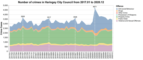
As depicted in Figure 4, Haringey’s crime composition and changes from 2017 to 2020 stayed similarly with three major types: property crimes, violence and sexual offenses, and anti-social behavior; the peak month from 2017 to 2019 was July, with crime volume at 3606, 3517, and 3548 respectively. In 2020, April saw the highest number of crimes at 4671, rising about 30% from the year-on-year peak values, which might be attributed to the surge of anti-social behaviors; but ironically, it also experienced the lowest number of property crimes. The general fluctuating trends in public order offenses, possession of weapons, and violence and sexual offenses had been consistent throughout the four years, with 2020 experiencing the greatest crime volatility apart from previous years’ trends. This study will take 2019, a typical normal year, as the benchmark, to analyze its crime data with that in 2020 for comparison.

Figure 4. Number of crimes in Haringey from 2017.01 to 2020.12.

4.1. Network autocorrelation of Haringey’s crime

Network autocorrelation considers the proximity and the similarity or disparity of values between two arcs, to evaluate the significance of the spatial dependence of the same variable. Since this study aims to detect crime patterns projected onto street network, the arc-based contiguity weight had been used to represent spatial closeness. From the scatter plot in Figure 5, a positive spatial autocorrelation had been observed, indicating that street segments with similar crime values tend to cluster. The p-value of Global Moran’s I is 0.12 (larger than 0.05), which means that the assumption of CSR cannot be rejected. It has been justified by the statistical value of the actual data (the red line) as reference for distribution.

Figure 5. The results of global Moran’s I.

LISA cluster maps based on local Moran’s I statistics (Figure 6), had presented the relationship between target location and its surrounding environment, and highlighted the crime “hot street” and “cold streets”. The “HH” streets (red segments in the left map) are streets with high crimes and surrounded by neighboring streets with high crimes; “LH” (legend in light blue) streets are those with low crimes but surrounded by neighbors with high crimes. Streets in gray (with the value of “ns”) had been taken as with spatially random distributed crimes.

Figure 6. The results of local spatial autocorrelation.

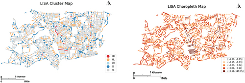
It is obvious that, crime patterns on certain streets had presented spatial autocorrelation, which further emphasized the importance to investigate crime patterns against street segments rather than areas, aiming for more accurate strategies and decision making on policing.

4.2. “Hot street” of crime

This study took all 4,923 street segments in Haringey as the targets, and assumed that (1) the crime density of a crime street is determined by both itself and the surrounding crime streets, (2) the crime-free street is only affected by the crime spillovers from neighboring crime streets. Upon applying the proposed algorithm, local crime “hot street” map could be 3D visualized in Figure 7. Note: the values of being “hot street” had been standardized from 0 to 1, to avoid magnitude variations by crime type. It had been interpreted that, a larger value on the street indicates a higher crime density.

Figure 7. Three-Dimensional visualisation of crime density in Haringey (2020 compared to 2019, zoom in on the value at a scale of 1 mile).

As presented in Figure 7, some street segments had experienced significant crime density changes in 2020 from 2019. For example, Brownlow Road (Area 1) had seen the most obvious crime decrease in 2020 by 68.75% comparing to 2019; High Road in Wood Green commercial center (Area 2) had seen crime reduction by 47.45%, while High Road in Northumberland Park (Area 4) saw crime reduction at 52.00% during 2020. Although most streets in Area 4 and Area 5 experienced similar crime drop trends in 2020, they presented unique feature in that, high crime streets incorporate roundabouts. Details on crime “hot streets” by crime type (six types) in 2020 and their year-on-year change to 2019 will be discussed hereafter, while the derived information on top ten crime “hot streets” in 2020 had been summarized in Table 5. In Figure 8, crime “hot streets” in Haringey in 2020 had been presented by type using the quartile scheme, while keeping those crime-free streets as a separate category; the corresponding counts of crime-free category and densest crime segments (“Hottest Street”) had been summarized in Table 3 for comparison. The crime changes against 2019 had also been drawn in Figure 9 by type, with most “hot streets” located to the east of the East Coast Main Line (an electrified railway). Property crimes had been found to be centered in the borough where the most notable “hot street” (High Road) is, which is also well-known as the home to local shopping center (The Mall Wood Green) attracting disrupting public order crimes. In parallel, violence and sexual offenses exhibited similar crime change pattern in Figure 9. Comparatively, antisocial behaviors were more dispersed distributed with the top 5 “hot streets” (Factory Lane, Stoneleigh Road, Wilson’s Avenue, Dowsett Road, and Honeysett Road) all located in the eastern of Haringey, namely Tottenham Hale area. It is one of the 11 wards in Haringey applying enforced alcohol control zones due to its most concerned anti-social behavior -street drinking -, which could not only cause public nuisances such as littering, noise, and urination, but also bring troubles to residents. Drug crimes were also found more stretched in the east, with two noticeable “hot streets”: (1) Wood Green High Road in the center, extending south from Green Lanes to Turnpike Lane; (2) High Road, borders with Bruce Grove and Tottenham Hale and crosses Tottenham Green. These two streets share the feature of being the main roads of traffic, as well as being the home to two drug markets (Wood Green Drug Market and Ducketts Common Drug Market) along the Wood Green High Road. As such, it could be inferred that Wood Green had experienced a significant number of drug offenses. Criminal behaviors of possessing offensive weapons are uncommon in Haringey, in the reflection of insignificant change at 76% of street segments. But the northeast ward (Northumberland Park) turned out to have several extremely “hot streets” for possessing offensive weapons, which are adjacent to each other and located in its retail and recreation region (Figure 2).

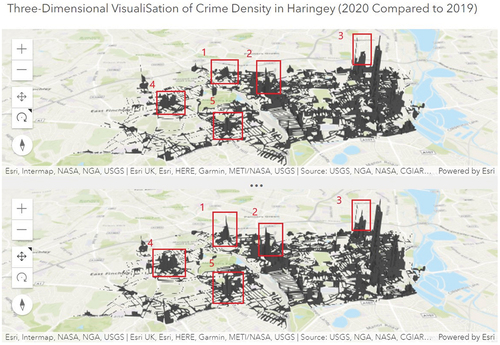
Figure 8. “Hot street” maps of different crimes in Haringey in 2020.

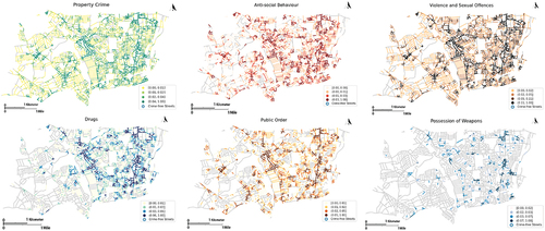
Figure 9. Crime change of different crimes in Haringey (2020 VS 2019).

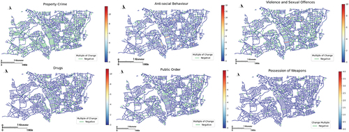
Table 3. Haringey’s number of street segments by different crime types.

Crime Type	Crime-free	“Hottest Street” of Crime
Property crimes	461	1116
Anti-social behaviour	680	1061
Violence and sexual offences	619	1076
Drug crimes	1845	770
Public order offences	1697	807
Possession of weapons	3767	289

4.3. Characteristics of “Hot street”

In recognition of “hot streets”, it is essential to investigate the features playing influential roles; hence 13 suggested variables consisting of 3 aspects, road properties, surrounding facilities, and contextual information, had been considered in the regression analysis. Upon applying the Backward Stepwise (BS) Regression technique (Smith 2018) to screen exposure variables, independent variables finally included in the models are: street length, carriageway width, CCTV cameras, traffic signals, IMD, average house price, average household income, and mobility change. Results for four regression models, the OLS model, the SL model, the SE model, and the GWR model, are shown in undefined 4. It is obvious that, the OLS model could only explain 16.89% of the variance of crime density using all independent variables, with Akaike’s Information Criterion (AIC) valued at 19,958.92. Since the smaller the AIC value is, the better the model fits, it could be found that the SL model or the SE model is better with a smaller AIC value (16,144.44 and 16,235.08 respectively). Such indication emphasized the importance of spatial effect on local crimes development, but also brought the attention to understand such a complicated topic against varied neighborhood features that substantially affect the crimes’ spatial patterns (Darmofal 2015), which requires discussing multivariate relations rather than only bivariate correlations. Comparing the four models’ performance in Table 4, the GWR model has been found the best fitted with a R-square at 0.744 and the AIC value at 11,483.71, especially incorporated the local perspectives in evaluating the spatial relations.

Table 4. Comparison of the results of four regression models.

Ordinary Least Squares Regression
Sum squared residual:		8852.566
Mean dependent var:	0.8495	R-squared:		0.1689
S.D. dependent var:	1.3042	Adjusted R-squared:		0.1679
Akaike info criterion:	19958.923	Schwarz criterion:		20,019.605
Maximum Likelihood Spatial Lag
Mean dependent var:	0.8495	Pseudo R-squared:		0.6184
S.D. dependent var:	1.3042	Spatial Pseudo R-squared:		0.0023
Akaike info criterion:	16,144.448	Schwarz criterion:		16,211.872
Maximum Likelihood Spatial Error
Mean dependent var:	0.8495	Pseudo R-squared:		0.1653
S.D. dependent var:	1.3042
Akaike info criterion:	16235.083	Schwarz criterion:		16,295.765
Geographically Weighted Regression
Spatial kernel:	Adaptive bisquare Bandwidth used:			59.000
Residual sum of squares:		1 602.686
R-squared:	0.744	AIC:		11,483.712
Adjusted R-squared:	0.688	AIC c:		11,975.162

Table 5. Top 10 “Hot street” of crime in 2020.

Property Crime	Anti-social Behaviour	Violence and Sexual Offence	Drugs	Public Order	Possession of Weapons
High Road (Wood Green)	Factory Lane	Reform Row	Neville Place	Reform Row	Fitzwarren Gardens
Cannon Road	Stoneleigh Road	Factory Lane	Bennetts Close	Dowsett Road	Grovelands Road
Factory Lane	Wilson’s Avenue	Dowsett Road	High Road (Wood Green)	Factory Lane	Bennetts Close
Reform Row	Dowsett Road	Hale Gardens	Cooperage Close	High Road (Tottenham)	The Hale
Dowsett Road	Honeysett Road High Road	The Hale	Roebuck Close	Stamford Hill	Hale Gardens
Gladstone Mews	(Bruce Grove/Tottenham)	Nevile Place	Northumbert and Park	Bennetts Close	Hale Road
Pelham Road	Bramble Close	High Cross Road	Portree Close	Portree Close	High Cross Road
Bennetts Close	Reform Row	Cannon Road	The Hale	Roebuck Close	Monument Way
Stoneleigh Road	White Hart Lane	Bennetts Close	Roebuck Close	Cooperage Close	High Road (Tottenham)
Ferry Lane	Bruce Grove	Monument Way	The Avenue	Neville Place	West Green Road

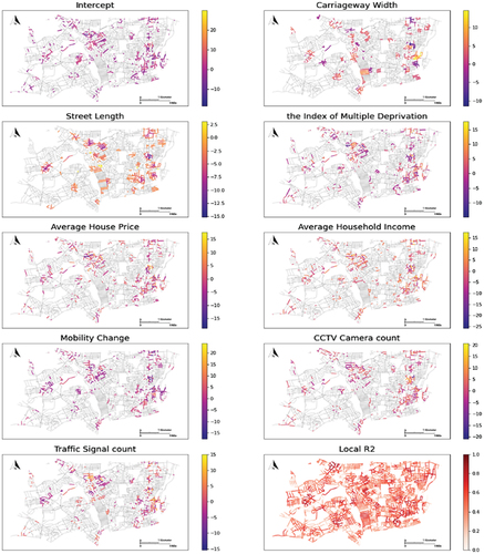
Results from GWR model in Figure 10 presented the impacts from each of the eight factors on local crime, where statistically insignificant street segments had been colored in gray, and brighter colors indicated significant crime influences. It is apparent that factor’s impacts on crime “hot streets” vary spatially in the target area, but with regional clustering patterns. It could hereafter be of reference to make targeted crime prevention strategies and corresponding crime deterrent measures. For instance, the “hot streets” being positively affected by carriageway width or street length indicators, could be suggested to introduce the Low Traffic Neighborhoods (LTN) (Goodman, and Aldred 2021) strategy, in order to restraint pedestrian and traffic flows to some extent toward the crime reduction purpose. Those hot streets overlapped with neighborhoods featured by low-income level, high unemployment rate and increased poverty, should call the attention from local police forces on implementing strengthened patrols and promoting more frequently on relevant laws and regulations. Security infrastructures, such as CCTV cameras and traffic lights, can also act as visible deterrents because their scientific installation alongside hot streets could provide extra surveillance locally.

Figure 10. Estimates of parameters and R-square of streets in Haringey estimates of parameters and R-square of streets in Haringey.

4.4. Lockdown impacts

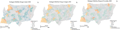
As discussed, the crime patterns in Haringey in 2020 averted from 2019 against COVID-19 pandemic, when the UK government has formulated regulations to prevent people from engaging in non-essential contact and travel. Such measures like maintaining social distance, restricting gatherings, and limiting the use of public transportation, had induced significant mobility change as depicted in Figure 11 (mobility change of Haringey’s main commercial and residential areas in April, August, and November 2020). As expected, the human mobility in retail and recreation areas decreased by between 11% and 21% in April, when rigid closure of non-essential stores implemented. In August, when the government eased travel restrictions up and encouraged dining out, a relatively less decrease in mobility by 8.2% had been witnessed; but it became severe again in November, when the second lockdown was implemented, while the mobility decreased by 15.1% to 10%. A polar phenomenon on mobility change had been emerged in residential areas as expected, being consistent with the encouragement of stay at home and work from home schemes since late March 2020. As such, most human activities had been restricted to the residential areas, resulting in the mobility increases up to 30%. In August, when travel control was at its most relaxed, the mobility change in residential areas saw a milder increase owing to people’s being more active in the commercial center, rather than around residential areas. In November, since residents more adapted to the lockdown policy, the mobility change did not vary too much from August’s pattern.

Figure 11. Haringey’s mobility change in April, August, and November 2020.

Despite of the spatial disparities among Haringey streets, it is also worthwhile to explore the temporal pattern of crime change from 2020 to 2019 against the lockdowns. Figure 12 had displayed the monthly crime changes on a year-on-year basis by crime type and indicated a clear lockdown timeline impact from the exhibited peaks and troughs of recorded crime incidents. For example, the property crimes had decreased from January to July, with more pronounced effects from first lockdown (took effect on 26 March 2020) in April by 38.04% and in May by 41.91%. These reductions had been attributed to the mobility reduces in the retail and recreation area, and the increase of mobility in residential area; in the fact of local measures on closing shopping malls, pubs, and other entertainment venues, which had been found to considerably reduce the opportunities for potential criminals committing crimes such as shoplifting, personal theft, and robbery.

Figure 12. Crime changes in Haringey (2020 VS 2019).

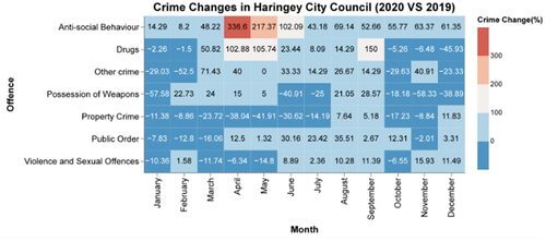
At the same time, people tend to spend more time at home, which contributed to the increased surveillance of their properties hence leading to less burglaries. Street crimes like violence and sexual offenses, public order offenses also saw declines about 10% during the lockdown periods (i.e. the former crime decreased by 11.4%, 6.34%, and 14.8% from March to May on monthly basis; the latter crime decreased by 16.06% in March but increased in the following months). The outbreak of anti-lockdown protests from April onwards was taken as being attributable to such crime shifts. The monthly anti-social behavior crimes increased in 2020 comparing with that in 2019, especially in April and May (about 3.4 times), which had related by academia to ethnicity and racial hate crimes, the Black Lives Matters campaigns fueled by the pandemic (Yeh 2020), as well as the surge in community complaints and quarrels among neighbors (Corry 2021). Drug-related crimes rocketed during the observation period, with approximately doubled in April and May, when self-isolation policy was well implemented, which was owed to those habitual drug users or groups with psychological problems (Williams 2021). Since the dine-out scheme rolled out in August, the number of all types of crime grew comparing to that in 2019, due to the ease up of travel restriction and the mobility increases’ enrichment of more potential crime targets. Although the second national lockdown was imposed in November, only possession of weapons crime had valued at the offenses experienced the largest increase at 15.93%.

5. Limitations

There are several limitations that should be noted for this research: (1) Time lag in crime recording and crime data missing: not only because of the nature of criminal legal procedures, but also due to the dark figure of crimes rendering less crimes been recorded than the actual occurrence. (2) Incomplete contextual data: the locational information on CCTV cameras and traffic signals had been distorted to ballpark values avoiding the geo-location privacy issue, which may result in some surveillance cameras being double counted. (3) Definition of street segments: a single street may be divided into several segments due to forks in the road. Moreover, in the crime “hot street” algorithm, the relationship between one street segment and other segments within the range may not be strictly “neighboring”, if there is no intersection between the two roads. (4) Data processing: the point-based crime data might be repeatedly counted when snapping crimes on the street, making a single crime case be counted by two nearest streets. (5) Hypothesis not convincing enough: some crimes, such as shoplifting, never being recorded on the streets by definition. Although we can figure out streets closest to such criminal activities, which may still carry out effective street patrols, it should be reconsidered in future research. (6) Co-integration issue: the BS method of screening the characteristics of crime “hot streets” may ignore the explanatory variables’ statistical significance when the confounding variables happened to be significant. This makes it possible for the model to fit well in-sample but not perform well out-of-sample (Smith 2018). (7) In addition, since the area studied in this paper is Haringey borough with an area at 29.58 square kilometers only, the sample size was relatively small, which in return limited the representativeness and capability to arrive at meaningful conclusions on finer scaled streets, as well as the impact of the national lockdown policy on specific crime hot streets.

6. Conclusions and future work

This study explored Haringey’s crime on individual streets in 2019 and 2020 and evaluated the impacts from lockdowns on crime patterns. The most prevalent types of crime were anti-social behavior (15932, 37%), property crimes (15555, 36%), violence and sexual offenses (7708, 18%), drug crimes (1803, 4%), public order offenses (1735, 4%), and possession of weapons (221, 1%). Their occurrence exhibited obvious local spatial autocorrelation. Factory Lane, Dowsett Road, Reform Row in the east, and High Road Wood Green in the center, were major crime “hot streets”, where the crimes accounting for the largest proportions were anti-social behaviors, public order offenses, violence and sexual offenses, and property crimes. To identify the characteristics of crime “hot streets”, eight factors are verified as significant independent variables: street length, carriageway width, CCTV cameras, traffic signals, IMD, average house price, average household income, and mobility change. Upon conducting GWR model to identify their relationships with crime, it had suggested that only certain factors had significant impacts on crimes at street level. Such findings were expected to provide more tailored guidance to local governors on localized crime deterrent measures, such as increasing the number of CCTV cameras and traffic signals on the streets of Factory Lane and Reform Row. Ever since the outbreak of the coronavirus pandemic in 2020, the crime density of “hot streets” had fluctuated along with the imposition and lifting of the lockdown policies. The most fundamental reason was that travel restrictions have led to people’s mobility change, reducing a lot of crime opportunities. With the introduction of the first lockdown policy at the end of March, property crimes in April decreased by about 38% comparing to 2019, and such shift could be observed clearly on streets located in commercial and residential areas. Upon encouraging the public to return to restaurants in August, the densities of all crimes had increased; when the second lockdown policy was enforced in November 2020, the crimes of possession of weapons (−58.33%), property crimes (−8.84%), and drug crimes (−6.48%) declined, but with increase of violence and sexual offenses by about 16%. Anti-social behavior in 2020 had increased monthly throughout the year, especially in April by about 3.4 times higher.

This study’s main contribution to literature is the crime hot streets algorithm, applying KDE and taking crime spillover effect into account on the assumption that, crimes along the streets are affected by themselves and the spillover effects from neighboring streets (within 100 meters) with crime presence; while those crime-free streets are only affected by crime streets within defined range. Such findings can be visualized as “hot street” maps by crime type, and further providing LEAs with more precise instructions on street patrolling, as well as more efficient policing assignments. Moreover, it has high flexibility for future toning in that, parameters can be adjusted easily, and the coupling is reduced to increase its maintainability. For example, the spatial matrix can instead use the driving distance or walking time to redefine “neighboring” streets. In practice, local government or the SCA team can modify the scope of crime spillovers from neighboring streets. Needless to say, the algorithm could be applied in multiple research fields, e.g. to identify roads with more frequent traffic accidents, to measure the impact on air quality from street trees.

In the future, there are still some areas for improvement. (1) The current research develops the algorithm only using one London borough as case study. It is worthwhile to apply and test the algorithm in varied contexts and cities. (2) Although current research is street-based, KDE method in this algorithm had been conducted on the network plane; if any future searching method in KDE can determine which neighboring streets are directly from street lengths, the algorithm would be more accurate. (3) In addition, this study attempted to build a new algorithm using Getis-Ord G* statistics, bearing importance with the comparison of two algorithms’ outcomes for practical crime-combating. (4) Finally, such research in relevant field could benefit more upon classifying the streets, in order to receive more detailed findings on specific crime types. For example, applying it onto the dominating crimes on motorways-smuggling and robberies-to suggest more applicable measures for transportation policing and avoiding potential crime spillovers.

Highlights

The novelty of the work can be summarised as follows.

1. A crime ”Hot Streets” algorithm using network-based KDE to analyse crime by types in one London Borough.

2. This is a timely and practical work for the local city council in formulating effective policies to conquer crime change in the short term, especially during the lockdown periods.

3. An attempt linking crime changes with human mobility changes during the lockdown periods, and a new calculation of human mobility change at the micro-level of different land uses.

Acknowledgements

The authors would like to thank Mr Broca Sandeep, the Intelligence Analysis Manager from the Haringey local authority, for providing valuable suggestions in this research.

Disclosure statement

No potential conflict of interest was reported by the author(s).

Data Availability Statement

Data available on request from the authors. The data that support the findings of this study are available from the corresponding author, upon reasonable request.

Additional information

Funding

This work is partly supported by King’s Global Engagement Partnership Fund [2020-2021 #PF2021_Mar_005].

Notes on contributors

Yuying Wu

Yuying Wu received her Master’s degree on Urban Informatics from CUSP London, Dept. of Informatics, King’s College London.

Yijing Li

Yijing Li is an Assistant Professor in CUSP London, Dept. of Informatics, King’s College London. She received the PhD degree from University of Cambridge. Her research interests are Geography of Crime, Spatial Analysis & Visualisation and Urban Data Mining.

References

- Andresen, M.A., and N. Malleson. 2010. “Testing the Stability of Crime Patterns: Implications for Theory and Policy.” The Journal of Research in Crime and Delinquency 48 (1): 58–82. doi:10.1177/0022427810384136.
- Angel, S. 1968. Discouraging Crime Through City Planning. Institute of Urban and Regional Development. Berkeley, CA: University of California: Center for Planning and Development Research.
- Anselin, L. 1988. “The Scope of Spatial Econometrics.” Spatial Econometrics: Methods and Models. Studies in Operational Regional Science, vol 4. 7–15. Springer, Dordrecht. https://doi.org/10.1007/978-94-015-7799-1_2
- Basile, R., M. Durbán, R. Mínguez, J.M. Montero, and J. Mur. 2014. “Modeling Regional Economic Dynamics: Spatial Dependence, Spatial Heterogeneity and Nonlinearities.” Journal of Economic Dynamics & Control 48: 229–245. doi:10.1016/j.jedc.2014.06.011.
- Black, W.R. 2010. “Network Autocorrelation in Transport Network and Flow Systems.” Geographical Analysis 24 (3): 207–222. doi:10.1111/j.1538-4632.1992.tb00262.x.
- Brantingham, P.J., and P.L. Brantingham. 1984. Patterns in Crime. New York: Macmillan.
- Brantingham, P.L., and P.J. Brantingham. 1993. “Nodes, Paths and Edges: Considerations on the Complexity of Crime and the Physical Environment.” Journal of Environmental Psychology 13 (1): 3–28. doi:10.1016/S0272-4944(05)80212-9.
- Brantingham, P.L., and P.J. Brantingham. 2010. “Notes on the Geometry of Crime (1981).” In Andresen, M.A., Brantingham, P.J., and Kinney, J.B., eds. Classics in Environmental Criminology (1st ed.), 247–272. Routledge. https://doi.org/10.4324/9781439817803
- Brantingham, P.J., and P.L. Brantingham. 2016. “The Geometry of Crime and Crime Pattern Theory.” In R. Wortley and M. Townsley, M. (eds). Environmental Criminology and Crime Analysis (2nd ed.), 117–135. London: Routledge. https://doi.org/10.4324/9781315709826
- Brunsdon, C., A.S. Fotheringham, and M. Charlton. 2002. “Geographically Weighted Summary Statistics–a Framework for Localised Exploratory Data Analysis.” Computers, Environment and Urban Systems 26 (6): 501–524. doi:10.1016/S0198-9715(01)00009-6.
- Caminha, C., V. Furtado, T.H. Pequeno, C. Ponte, H.P. Melo, E.A. Oliveira, and J.S. Andrade. 2017. “Human Mobility in Large Cities as a Proxy for Crime.” Plos One 12 (2): e0171609. doi:10.1371/journal.pone.0171609.
- Cheung, L., and P. Gunby. 2021. “Crime and Mobility During the Covid-19 Lockdown: A Preliminary Empirical Exploration”. New Zealand Economic Papers, 1–8.
- Cohen, L.E., and M. Felson. 1979. “Social Change and Crime Rate Trends: A Routine Activity Approach.” American Sociological Review 44 (4): 588–608. doi:10.2307/2094589.
- Corry, K. 2021. “Surge in Noise Complaints in London During the First Lockdown”. Accessed 21 September 2021. https://www.ucl.ac.uk/news/2021/may/surge-noise-complaints-london-during-first-lockdown
- Darmofal, D. 2015. Spatial Analysis for the Social Sciences. New York: Cambridge University Press.
- Eck, J.E., S. Chainey, J.G. Cameron, M. Leitner, and R.E. Wilson. 2005. Mapping Crime: Understanding Hotspots. USA: U.S. Department of Justice Office of Justice Programs National Institute of Justice.
- Eck, J.E., R.V. Clarke, and R.T. Guerette. 2007. “Risky Facilities: Crime Concentration in Homogeneous Sets of Establishments and Facilities.” Crime Prevention Studies 21: 225.
- Flatley, J. 2016. “Focus on property crime: Year ending March 2016”. Accessed 21 September 2021. https://www.ons.gov.uk/peoplepopulationandcommunity/crimeandjustice/bulletins/focusonpropertycrime/yearendingmarch2016
- Goodman, A., and R. Aldred. 2021. “The Impact of Introducing a Low Traffic Neighbourhood on Street Crime, in Waltham Forest, London”. Findings.
- Harries, K. 1999. Mapping Crime: Principle and Practice. National Institute of Justice, US Dept. of Justice Office of Justice Programs, Washington DC.
- Hauer, E. 1997. Observational Before–after Studies in Road Safety: Estimating the Effect of Highway and Traffic Engineering Measures on Road Safety. Oxford: Elsevier Science Ltd.
- Hauer, E., D.W. Harwood, F.M. Council, and M.S. Griffith. 2002. “Estimating Safety by the Empirical Bayes Method: A Tutorial.” Transportation Research Record: Journal of the Transportation Research Board 1784 (1): 126–131. doi:10.3141/1784-16.
- La Vigne, N.G. 1996. “Safe Transport: Security by Design on the Washington Metro.” Preventing Mass Transit Crime 6: 163–197.
- Lee, M., and P. Holme. 2015. “Relating Land Use and Human Intra-City Mobility.” Plos One 10 (10): e0140152. https://doi.org/10.1371/journal.pone.0140152
- Lowman, J., G. Rengert, and J. Wasilchick. 1987. “Suburban Burglary: A Time and a Place for Everything.” Economic Geography 63 (1): 96. doi:10.2307/143863.
- Milić, N., Z. Ðurđević, S. Mijalković, and E. Erkić. 2020. “Identifying Street Hotspots Using a Network Kernel Density Estimation.” Revija Za Kriminalistiko in Kriminologijo/ljubljana 71 (4): 257–272.
- Mitra, S. 2009. “Spatial Autocorrelation and Bayesian Spatial Statistical Method for Analyzing Intersections Prone to Injury Crashes.” Transportation Research Record: Journal of the Transportation Research Board 2136 (1): 92–100. doi:10.3141/2136-11.
- O’-Brien, D.T. 2018. “The Action is Everywhere, but Greater at More Localized Spatial Scales: Comparing Concentrations of Crime Across Addresses, Streets, and Neighborhoods.” The Journal of Research in Crime and Delinquency 56 (3): 339–377. doi:10.1177/0022427818806040.
- Paisley, J. 2017. “Use Spatial Sciences Students Analyze Crime Patterns in L.A.” Accessed 21 September 2021. https://news.usc.edu/115324/usc-spatial-sciences-students-analyze-crime-patterns-in-l-a/
- Parzen, E. 1962. “On Estimation of a Probability Density Function and Mode.” The Annals of Mathematical Statistics 33 (3): 1065–1076. doi:10.1214/aoms/1177704472.
- Poulsen, E., and G. Birchall. 2002. “Designing a Database for Law Enforcement Agencies.” In Leipnik, M.R., and Albert, D.P., eds. GIS in Law Enforcement: Implementation Issues and Case Studies (1st ed.), 85–96. Routledge. https://doi.org/10.1201/9780203217955
- Prathap, B.R., and K. Ramesha. 2020. “Geospatial Crime Analysis to Determine Crime Density Using Kernel Density Estimation for the Indian Context.” Journal of Computational and Theoretical Nanoscience 17 (1): 74–86. doi:10.1166/jctn.2020.8632.
- Reiss, A.J., and D.P. Farrington. 1991. “Advancing Knowledge About Cooffending: Results from a Prospective Longitudinal Survey of London Males.” The Journal of Criminal Law & Criminology 82 (2): 360. doi:10.2307/1143811.
- Rosser, G., T. Davies, K.J. Bowers, S.D. Johnson, T. Cheng, et al. 2017. ”Predictive Crime Mapping: Arbitrary Grids or Street Networks?” Journal of Quantitative Criminology 33 (3): 569–594. https://doi.org/10.1007/s10940-016-9321-x
- Shiode, S., and N. Shiode. 2013. “Network-Based Space-Time Search-Window Technique for Hotspot Detection of Street-Level Crime Incidents.” International Journal of Geographical Information Science 27 (5): 866–882. doi:10.1080/13658816.2012.724175.
- Smith, G. 2018. “Step Away from Stepwise.” Journal of Big Data 5 (1). doi:10.1186/s40537-018-0143-6.
- Stickle, B., and M. Felson. 2020. “Crime Rates in a Pandemic: The Largest Criminological Experiment in History.” American Journal of Criminal Justice 45 (4): 525–536. doi:10.1007/s12103-020-09546-0.
- Taylor, R.B. 1997. “Social Order and Disorder of Street Blocks and Neighborhoods: Ecology, Microecology, and the Systemic Model of Social Disorganization.” The Journal of Research in Crime and Delinquency 34 (1): 113–155. doi:10.1177/0022427897034001006.
- Taylor, R.B., S.D. Gottfredson, and S. Brower. 1984. “Block Crime and Fear: Defensible Space, Local Social Ties, and Territorial Functioning.” The Journal of Research in Crime and Delinquency 21 (4): 303–331. doi:10.1177/0022427884021004003.
- Tom-Jack, Q.T., J.M. Bernstein, and L.C. Loyola. 2019. “The Role of Geoprocessing in Mapping Crime Using Hot Streets.” ISPRS International Journal of Geo-Information 8 (12): 540. doi:10.3390/ijgi8120540.
- Tompson, L., H. Partridge, and N. Shepherd. 2009. “Hot Routes: Developing a New Technique for the Spatial Analysis of Crime.” Crime Mapping: A Journal of Research and Practice 1 (1): 77–96.
- Wagner, A.E. 1997. “A Study of Traffic Pattern Modifications in an Urban Crime Prevention Program.” Journal of Criminal Justice 25 (1): 19–30. doi:10.1016/S0047-2352(96)00048-7.
- Weisburd, D., S. Bushway, C. Lum, and S.M. Yang. 2004. “Trajectories of Crime at Places: A Longitudinal Study of Street Segments in the City of Seattle.” Criminology 42 (2): 283–322.
- Weisburd, D., and L. Green. 1995. “Policing Drug Hot Spots: The Jersey City Drug Market Analysis Experiment.” Justice Quarterly 12 (4): 711–735. doi:10.1080/07418829500096261.
- Weisburd, D., E. Groff, and S.M. Yang. 2013. The Criminology of Place Street Segments and Our Understanding of the Crime Problem. Oxford, UK: Oxford University Press.
- Weisburd, D., and L.G. Mazerolle. 2000. “Crime and Disorder in Drug Hot Spots: Implications for Theory and Practice in Policing.” Police Quarterly 3 (3): 331–349. doi:10.1177/1098611100003003006.
- Williams, N. 2021. “How Has the Covid-19 Pandemic Affected Recreational Drug Use”. Accessed 21 September 2021. https://www.news-medical.net/health/How-has-the-COVID-19-Pandemic-affected-Recreational-Drug-Use.aspx.
- Wisniewski, M., and J.O. Rawlings. 1990. “Applied Regression Analysis: A Research Tool.” The Journal of the Operational Research Society 41 (8): 782. doi:10.1057/jors.1990.106.
- Xie, Z., and J. Yan. 2008. “Kernel Density Estimation of Traffic Accidents in a Network Space.” Computers, Environment and Urban Systems 32 (5): 396–406. doi:10.1016/j.compenvurbsys.2008.05.001.
- Yeh, D. 2020. “Covid-19, Anti-Asian Racial Violence, and the Borders of Chineseness.” British Journal of Chinese Studies 10. doi:10.51661/bjocs.v10i0.117.