Mapping of cropland, cropping patterns and crop types by combining optical remote sensing images with decision tree classifier and random forest

ABSTRACT

Mapping and monitoring the distribution of croplands and crop types support policymakers and international organizations by reducing the risks to food security, notably from climate change and, for that purpose, remote sensing is routinely used. However, identifying specific crop types, cropland, and cropping patterns using space-based observations is challenging because different crop types and cropping patterns have similarity spectral signatures. This study applied a methodology to identify cropland and specific crop types, including tobacco, wheat, barley, and gram, as well as the following cropping patterns: wheat-tobacco, wheat-gram, wheat-barley, and wheat-maize, which are common in Gujranwala District, Pakistan, the study region. The methodology consists of combining optical remote sensing images from Sentinel-2 and Landsat-8 with Machine Learning (ML) methods, namely a Decision Tree Classifier (DTC) and a Random Forest (RF) algorithm. The best time-periods for differentiating cropland from other land cover types were identified, and then Sentinel-2 and Landsat 8 NDVI-based time-series were linked to phenological parameters to determine the different crop types and cropping patterns over the study region using their temporal indices and ML algorithms. The methodology was subsequently evaluated using Landsat images, crop statistical data for 2020 and 2021, and field data on cropping patterns. The results highlight the high level of accuracy of the methodological approach presented using Sentinel-2 and Landsat-8 images, together with ML techniques, for mapping not only the distribution of cropland, but also crop types and cropping patterns when validated at the county level. These results reveal that this methodology has benefits for monitoring and evaluating food security in Pakistan, adding to the evidence base of other studies on the use of remote sensing to identify crop types and cropping patterns in other countries.

KEYWORDS:

• Sentinel-2
• Random Forest
• cropland
• crop types
• cropping patterns
• Decision Tree Classifier

1. Introduction

Food security is a key problem the world is facing due to a rapidly increasing population and climate change. According to a Report published by the Food and Agriculture Organization (FAO), approximately 815 million people worldwide were undernourished in 2016, an 11% increase from the previous year (FAO 2017). Moreover, the global population is projected to grow to over 7.9 billion, 9.7 billion, and 11.2 billion people by 2030, 2050, and 2100, respectively (UN 2015). This population growth will put further pressure on natural resources, notably to meet the growing demand for food (Lambert, Waldner, and Defourny 2016). Technological development for mapping and monitoring croplands will become essential to overcome the challenge of food security and thus to address the United Nations Sustainable Development Goal of no poverty and zero hunger, with the latter organization encouraging the use of available technologies to meet this purpose (UN 2015).

Monitoring crop conditions is central to agricultural policies and decision-making, but this requires high-quality and up-to-date datasets. Remote sensing has been used for this purpose, notably for allocating farm subsidies in Europe, forecasting crop yields in Europe and North Africa, and developing early warning systems for food security (Bellón et al. 2017). In Pakistan, the agricultural production has increased significantly in the past three decades (Hamza et al. 2021), and the agricultural sector is now an indispensable part of the economy, employing about 40% of the population (Al-Qaness et al. 2022; Hussain et al. 2022). Several studies have previously been conducted to map the distribution of agricultural activities in Pakistan (Das, Zhang, and Ren 2022; Imran et al. 2022; Tariq et al. 2021), but a monitoring system is still needed, and remote sensing could facilitate its development.

Satellite images together with phenological information have previously been used to retrieve information on the extent of cropland and the type of crops and cropping patterns across different regions (Sanyal and Lu 2004; Yang, Zhao, and Chan 2018). The Landsat satellite images, in particular, are widely used for crop mapping because they are freely available, their spatial resolution is reasonably good, and they have been available since 1972 (Kulkarni 2017). Landsat images, however, are only available every 16 days, plus some of them cannot be used due to the presences of clouds; consequently, they are not the best remote sensing product for continuous monitoring of crops during their growth period. Alternatively, some studies have used images from the Moderate Resolution Imaging Spectroradiometer (MODIS) or a combination of Landsat and MODIS data given the high temporal frequency albeit low horizontal resolution of the latter (Kumar and Parikh 2001; Samboko et al. 2020; Thenkabail and Gamage 2004). In recent studies, Sentinel-2 makes the probability of relating Decision Tree Classification (DTC) and Random Forest (RF) to extract crop types from time-series data of sentinel-2 data. Moreover, crop classification has also been done using the Sentinel-2 Enhanced Vegetation Index (EVI) and the Normalized Difference Vegetation Index (NDVI) time-series data (DeFries and Townshend 1994; Gu et al. 2007; Han, Wang, and Zhao 2010) using either subpixel and pixel-based methods. These researches have all concentrated on classifying multi-temporal images at the pixel level as their primary objective.

Machine Learning (ML) techniques have become more widely used in agriculture, particularly to improve the productivity and quality of crops. Random Forest (RF), for instance, is an ensemble learning classifier (Chen et al. 2018) that has achieved excellent results in cropland mapping (Hou, Wang, and Murayama 2019; Novelli et al. 2017; Youssef et al. 2016). The latter was used by (Pelletier et al. 2016) for land cover mapping, including the delineation of agricultural fields using pan-sharpened Pléiades images at a 0.5-m resolution. Additional information such as altitude and slope were used to classify the fields using reflectance and spectral indices calculated with Sentinel-2 (artificially constructed images from SPOT-5) and Landsat 8 (OLI/TIRS images) and DEM-based auxiliary information. In order to categorize greenhouse segments from WorldView-2 images, (Novelli et al. 2017) utilized single-date Sentinel-2 and Landsat 8 data. (Liu et al. 2014; Nicolaou and Shane 2010) described a multi-temporal object-based technique for mapping cereal crops using Landsat SLC-off ETM+ images (without using gap-filling schemes). There were no mixed-crop classifications of fields due to the salt-and-pepper effect associated with a pixel-based technique, which is common when classifying fields using multiple data sources.

The above-mentioned studies focused on classifying time-series images using RF and DTC methods. According to Petitjean et al. (2012), the increasing spatial resolution of available space-borne sensors, such as the Multispectral Imager sensor (MSI) on Sentinel-2, allows for RF analysis to derive crop types from many series of data. RF is a tree-based classifier, which means that many trees are constructed, and then those trees are joined based on an equally weighted majority vote. When training a certain tree, it is typical practice to leave out one-third of the original training dataset on a purely random basis.

This study presents a methodology using the Sentinel-2 and Landsat-8 data along with ML techniques to first map the distribution of cropland in the Gujranwala region of Pakistan and second to identify the main crop types and cropping patterns in the region (i.e. the planting combinations of different crop types in a given area within an agricultural period): wheat-tobacco, wheat-barley, and wheat-gram. The accuracy of the methodological approach presented in this paper is then assessed.

2. Materials and methods

2.1. Study area

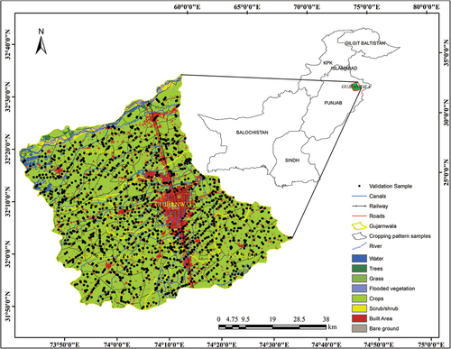
This study focuses on the irrigated part of the Chenab River basin in the Gujranwala District of Punjab Province, Pakistan, which encompasses an area approximately 3654.24 km² in size (Figure 1). The district is an important agricultural region in Pakistan; it is the fifth largest agricultural district in the country and one of the regions producing the most wheat. There are two dominant cropping seasons in the region, which are commonly known as the summer or rainy season, beginning in May and ending in October. The winter season where the sowing starts in November and the harvest takes place by late April. The land cover types vary considerably in the district due to variation in topography, soils, and climate (Imran et al. 2018), as shown in Figure 1. Mean annual temperature is 23.9°C and total annual precipitation is 578 mm (Liaqut et al. 2019; Salma, Rehman, and Shah 2012).

Figure 1. Land Use/Land Cover (LULC) types of the study areas with location of validation samples.

2.2. Data and processing of satellite images

Table 1 summarizes the datasets used in this study, which include satellite images, field survey, and statistical data about crop types. The images from Sentinel-2 (Level-1C S2) were downloaded from the Sentinel Scientific Data Center of the European Space Agency (ESA) (https://scihub.copernicus.eu), and processed using sen2cor plugin v2.8.0 tools in SNAP v5.0 (Muller-Wilm et al. 2013). ERDAS Imagine 2016 was used for classifying the Landsat images. The shapefile of the corresponding areas and mask were generated to extract the area of interest using ArcMap 10.8. The Landsat 8 images were processed using ENVI 5.4 and ArcMap. Sample plots were located with the help of the Global Positioning System (GPS).

Table 1. Datasets used in the study.

Data Acquisition	Spatial Resolution	Temporal Resolution	Time Period	Source
Sentinel-2 LULC types	10 m	Yearly	2020	https://scihub.copernicus.eu/
Sentinel-2 (MSI)	10 m	5 days	From August 2015 to December 2018	https://scihub.copernicus.eu/
Landsat 8 (OLI/TIRS)	30 m	16 days	August 2015 and December 2021	https://earthexplorer.usgs.gov/
Land cover and cropping pattern samples	… …	… …	2020–2021	Field survey in August 2020-September 2021, Google Earth images
Crop type area statistics	184 samples	Yearly	2020–2021	http://www.amis.pk/

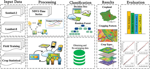
Figure 2 illustrates the research methodology from the acquisition of the Sentinel-2/Landsat-8 images to mapping cropland, crop types, and patterns. Persistent cloud cover throughout the rainfall season is a challenge to the use of optical remote sensing imagery in the study region, altering the actual land surface reflectivity. The pixel reliability band was used to detect clouds and shadows, and the affected pixels were removed. As Chen et al. (2018) explained, a temporal interpolation method was used to substitute the values of the cloud-contaminated pixels. These images (Sentinel-2/Landsat-8) were georeferenced into the same map projection of the World Geodetic System 1984 Zone 43°N (Tadesse et al. 2017). All satellite images were sub-mapped (subset) for covering only the study area. All satellite images were composed using red, green, and blue (RGB) color.

Figure 2. Flow chart representing the research methodology.

In order to generate the dense spectral time series, we combined images from the Operational Land Imager (OLI) onboard Landsat-8, which were available as Level 1, Collection 1, Tier 1 datasets, with images from the Multi-Spectral Instrument (MSI) onboard Sentinel-2A and S-2B, which were available as Level 1C data. Both sets of datasets were available from the European Space Agency. We selected temporal images with zero or close to zero (less than 10%) cloud coverage, taken between August 2015 and December 2021 for the study region, only visible bands 2, 3, and 4, and the near-infrared band (band 8) of Sentinel-2 data were used. Sentinel-2 reflectance images were transferred from Top-Of-Atmosphere (TOA) Level 1C Sentinel-2 to Bottom-Of-Atmosphere (BOA) Level 2A.

Radiometric topographic, atmospheric correction, and adjacency effect correction was performed with the FORCE Level-2 module (Seelan et al. 2003). Clouds and shadows were masked based on the optimized FMASK algorithm (Margono et al. 2012). In the study, Sentinel-2 and Landsat-8 images were used together with machine learning (DTC and RF) methods. We used Landsat-8 images with Sentinel-2 for the identification of cropland, cropping patterns, and crop types. Landsat-8 has a 30 m spatial resolution and Sentinel-2 has a 10 m spatial resolution. We converted spatial resolution of Landsat-8 to Sentinel-2. We need to fix this issue using STARFM technique. The Sentinel-2 bands with a 20 m spatial resolution were sharpened to 10 m using the spectral-only setup of the Spatial and Temporal Adaptive Reflectance Fusion Model (STARFM) technique (Belgiu, and Csillik 2018; Gao et al. 2006). The 30 m spatial resolution Landsat-8 bands were matched to the 10 m Sentinel-2 pixel grid using nearest neighbor resampling. According to Gao et al. (2006), STARFM is a popular method for spatio-temporal image fusion. Recent studies in this field are beginning to use deep learning methodologies, following the trend in computer vision research. Three recent image fusion research that used deep learning were identified by Dian et al. (2018), Ma et al. (2019), Palsson, Sveinsson, and Ulfarsson (2017), and Yang, Zhao, and Chan (2018). Spatial information weighting is an important aspect when STARFM is actually implemented. The study area’s complexity and heterogeneity determine how the weighting function is set. There are three steps to SATRFM, including spectrally similar neighbor pixels, a combined weighting function, and sample filtering.

1. Neighboring pixels that have comparable spectral information can be used to determine the right spectral information. Pixels can be obtained in two different methods. Pixels of the same class can be blended together before an unsupervised classification is done. Each and every Landsat image should be subjected to the unsupervised classification method. In order to capture surface changes at fine resolution and predict changes across dates, these spectrally similar neighbor pixels may differ from one time to the next, making them valuable for comparing changes over time. Surface reflectance thresholds can be used directly to detect spectrally comparable pixels. The STARFM algorithm can be used to incorporate the search process.

2. Spectrally similar pixels have their ultimate weights determined by three variables. They are based on the assumptions that: (a) the coarse-resolution homogeneous pixels provide the same temporal changes as fine-resolution observations from the same spectral class; (b) the observations with less change from the prediction date provide better information for the prediction date; and (c) the more proximal neighboring pixels usually provide better information for prediction. The last step in making the best weight function is to include both temporal and geographical information in the weight function.

3. It will be necessary to perform additional filtering on the candidates in order to eliminate low-quality observations after spectrally comparable pixels from high-resolution imageries have been picked. Second, pixels near the moving window are discarded if the central pixel’s spectral and spatial information is superior to that of the nearest neighboring pixels. It is rare for the forecast to be improved by the presence of an inferior neighbor pixel.

However, the pan-sharpening method aim to develop the spatial resolution of a single image by using a high spatial resolution band known as the panchromatic band to achieve this goal. An image fusion study, (Ghamisi et al. 2019) can also be characterized as a pan sharpening study in the perspective that they fuse low spatial resolution bands with panchromatic bands to produce high spatial resolution bands. A move toward deep learning is evident in this field, just with image fusion. A total of seven experiments utilizing deep learning for pan-sharpening have been documented (Belgiu and Stein 2019; Dian et al. 2018; Ghamisi et al. 2019; Isa et al. 2021; Ma et al. 2019; Palsson, Sveinsson, and Ulfarsson 2017; Yang, Zhao, and Chan 2018). In addition, we discovered two further deep-learning-based studies on pan-sharpening (Ghamisi et al. 2019). Super-resolution studies aim to improve an image’s spatial resolution in the same way as pan sharpening. A super-resolution model, on the other hand, does not make use of the panchromatic band. Super-resolution models in computer vision research are heavily affected by the Fully Convolutional Network (FCN) models, which are based primarily (FCN) (Ma et al. 2019).

The crop area derived from Sentinel-2 data was validated using the Landsat-8 images taken from August 2015 and December 2021, and because they have been terrain-corrected, they have excellent geometric accuracy. The Landsat-8 images were calibrated to spectral reflectance at the top of the atmosphere using the methodology described in (Mishra and Singh 2010). Then, the land surface reflectance was computed (Chander, Markham, and Helder 2009; Owojori and Xie 2005).

2.3. Ground validation

In addition to using the Landsat images, the validation of the cropland areas was performed using 1150 points chosen by random stratified sampling for each image. This revealed that the methodology described above to identify cropland areas from the Sentinel-2 images resulted in maps with an overall high accuracy (>80%) as well as good user and producer accuracy (>90%). Land-cover (LC) samples were chosen with the help of geotagged photos from field surveys and were used to identify LC categories using Sentinel-2 satellite-derived data between August 2015 and December 2021. An overall total of 1150 samples were gathered, including at least 50 samples from each land cover category. In August 2020 and September 2021, field surveys were conducted in the study area to gather crop-type samples. For training, 184 cropping pattern samples were collected, with at least 10 samples per cropping pattern. Statistical statistics for crop types comprise Tobacco, Wheat, Barley, and Gram for the 2020–2021 growing season. This information originated based from a survey, including statistics at the sub-district level.

2.4. Classification methods

2.4.1. Decision Tree Classifier (DTC)

There are a variety of classification methods available, including Artificial Neural-Network (ANN), MLC, Decision-Tree-Classifier (DTC), Random Forest (RF), and Support-Vector-Machine (SVM) (Lu and Weng 2007), with DTC considered the best method in land-cover categorization (Pan et al. 2003). DTC is considerably simpler and can be constructed from direct examination of variables than other machine-learning techniques, such as SVM and ANN, which require a lot of time and effort in training the classifier to get the optimal parameters. In terms of parameter pre-defining, outcome voting, and sample training, RF is more complicated than DTC since it is an ensemble of decision trees (Breiman 2001). Another benefit of DTC is that it has a clear operating machine based on training samples. DTC was created in MATLAB. Identifying appropriate variables and associated thresholds for each variable is a crucial step in DTC. A comparative study of several phenological metrics and temporal indices was performed to identify factors.

Previous studies have found that phenology characteristics are useful for land cover categorization (Pandya et al. 2013; Xu and Guo 2014; Zhao and Chen 2005). Six land cover categories were evaluated for each sample based on their NDVI temporal patterns, and the NDVI time series and the TIMESAT package were used to compute six phenological metrics (Hentze, Thonfeld, and Menz 2016). The maximum value, amplitude, at the start of the season, at the end of the season, based-values, and growing season duration are some of these measures. The beginning of the season is the point on the temporal curve when the distance between the left minimum and maximum levels is 15% of the distance between the left minimum and the maximum. On the other hand, the end of the season refers to the point on the temporal curve where the distance between the right minimum and the maximum value is 15% of the distance between the maximum value and the right minimum. The time gap between the start of the season and the end of the season refers to the growing season length. The difference in NDVI between the highest NDVI values and the base value is known as the amplitude (Jönsson and Eklundh 2004).

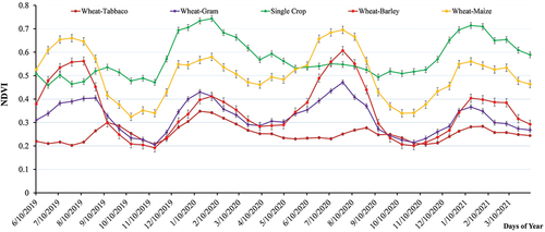
The temporal profile of the NDVI mean value for each Land Cover (LC) type is shown in Figure 3. To distinguish one LC type from another, many measurements in time need to be utilized. Although NDVI measurements may quickly determine land covered by forests from rivers and lakes during the dry season, this is not the case for separating agriculture from other land cover types or distinguishing one crop type from another. Like water and ISA, the crop has a considerably greater maximum value but is blended with other LCs. The crops are separated from nearly all other LC in terms of amplitude. As a result, amplitude and NDVI-dry were chosen because they offered the best potential for the differentiation of land cover types. The DTC was then developed to extract crops using NDVI-dry and amplitude as parameters. NDVI-dry was combined using the normal NDVI of total period facts from August. The NDVI-dry threshold was set at 0.25. This chosen was chosen as it is in the middle of the top and lower bounds of water and crops. Correspondingly, the amplitude threshold was customary at 0.38, chosen as the value midway between the cropped lowest and the water higher bounds. Finally, the DTC was used to create the agricultural zones in 2020 and 2021.

Figure 3. Temporal profiles for various cropping patterns in Gujranwala, Pakistan.

2.4.2. Random Forest classification

The RF algorithm is a classification method that is based on trees and involves the production of several trees that are then integrated using an equally weighted majority vote. During the process of training each individual tree, a third of the initial dataset that was used for training is omitted at random. RF is an ensemble learning classifier (Chuvieco, Martin, and Palacios 2002) that has achieved efficient classification results in a variety of remote sensing experiments, including farmland mapping. These results can be found in a variety of publications (Chen et al. 2018; Guru, Seshan, and Bera 2017; Hentze, Thonfeld, and Menz 2016). (Karnieli et al. 2010; Naveendrakumar et al. 2019), both provide a comprehensive analysis of RF technique as well as its usefulness in the field of remote sensing. In the course of our research, RF was executed with the help of a script based on the RF (v.4.6–12) R package (Millard and Richardson 2015).

2.5. Crop pattern and crop type mapping

Three phases of cops, including sowing, growing, and harvesting, were used to extract cropping patterns as each cropping pattern has its unique cycle. Crop phenology (temporal) profile is critical for crop type mapping. Figure 3 shows the NDVI temporal profiles in Gujranwala based on cropland and cropping patterns. While some cropping patterns have identical NDVI values at different times, particular distinctions may be utilized to identify these, such as sole cropping pattern classification having just a single top peak. However, a dual cropping pattern system has double heights. The highest peak values of the Wheat-Maize configuration through its unplanted period is significantly lower than the extra three dual cropping systems over the identical time, suggesting that the first season’s peak value is a possible variable to extract the peak value in the first season Wheat-Barley pattern. Because the NDVI values of Wheat-Tobacco in the dry season are considerably greater than that of Wheat-Maize, Wheat-Barley, and Wheat-Gram simultaneously, this value may be used to distinguish Wheat Tobacco from other patterns. Wheat-Barley harvest occurs earlier than Wheat-Maize, Wheat-Gram, and Barley harvest, subsequent in lesser NDVI values of Wheat-Tobacco than others throughout the identical time.

In contrast, Maize reap occurs earlier than barley harvest in Wheat-Maize and vegetation senescence in Wheat-Maize in the second crop season, resulting in lesser NDVI values of Wheat-Maize than others during the equal time. As a result, after the first and second crops season, NDVI data may be utilized as possible factors. It is substance mentioning that all edges were fine-tuned by altering their standards inside a positive variety defined by cropping pattern NDVI series.

All thresholds were fine-tuned by altering their values within a specific range defined by cropping pattern NDVI ranges. Following the implementation of the planned DTC, cropping pattern maps for the agricultural years 2020 and 2021 were created. While single Wheat and single barley have co-existed in Gujranwala in latest years, Wheat was used to define the single cropping system in this research. This is because (1) the barley and maize crops planted areas accounted for only 6% and 5% of total crop area, respectively, according to statistical data from 2020 to 2021, that single crop maize’s planted area is smaller than single barley’s and first crop maize’s ones; and (2) there are too many tiny patches of maize to classify. As a result of the same reasoning, additional dual cropping pattern systems, such as Wheat-Gram, were also eliminated from this study. These conventions are present in (Browning and Duniway 2011) as well. Section delves further into the uncertainties and biases arising from these assumptions.

2.6. Accuracy assessment

Image classification is challenging when working with images with a coarse spatial resolution because of the heterogeneity in LULC types, and uncertainties and errors inevitably arise. A matrix of error was used in this study, which is a common procedure to assess the uncertainties and biases in the results of image classification (Gumma et al. 2020). As previously mentioned, the assessment of the accuracy in the Sentinel-2 image classification to create cropland and crop types maps for the year 2015–2021 was performed using Landsat-8 images on the one hand and crop statistics on the other hand. The reliability of the various test samples and the procedure for allocating certain samples is crucial to an accuracy assessment (Mousa et al. 2020), with the focus normally on the estimated accuracy percentage and permissible error (Landerer, and Swenson 2012).

The amount of test samples generally usually dependent on the expected accuracy of the percentage usually depends on the expected percentage accuracy and acceptable mistakes (Landerer, and Swenson 2012) or on the thumb rule, which requires at least 50 test samples per class. The majority in this study aggregated the non-crop/crop data from Landsat-8 (30 m) cell size with a 10 m cell size, identical to Sentinal-2 data. One thousand one hundred and fifty test samples were chosen in all sub-districts using the stratified random sampling method from the aggregated crop distribution from imagery. These test samples were used for assessing agricultural maps generated from Sentinel-2 and Landsat-8. A total of 1151 test samples (obtained from all administrative units viz. Gujranwala, Kamoke, Nowshervirkhan, and Wazirabad, respectively) were chosen from gathered images of crop distribution stratified random sampling method. The Sentinel-2 and Landsat-8 cropland maps were evaluated using these test samples.

The error matrix for cropland was then established, and the result of the crop type classification, respectively. Another method for comparative evaluating the results extracted from Sentinel-2 was using administrative (county) level crop statistical data. For each county, the reference results were determined for crop type and cropland areas. For every county in Gujranwala, Sentinel-2 related crop type, cropping patterns and cropland areas were estimated utilizing a statistical zoning method. The NDAI, the adjusted determination coefficient ($R^2$), and the relative root means square-error (RRMSE) (Hentze, Thonfeld, and Menz 2016) were used to determine the Sentinel-2 outcomes explained in the following Equations (1–4):

(1) $\mathrm{N}\mathrm{D}\mathrm{A}{\mathrm{I}}_i=\left(E_i-S_i\right)$(1)

(2) $R^{\prime 2}=1-\sum _{i=1}^n{\left(E_i-S_i\right)}^2/\sum _{\mathrm{i}=1}^n{\left(E_i-\bar{S}\right)}^2\hspace{0.17em}$(2)

(3) $R^2=1-\left(1-{\mathrm{R}}^{\prime 2}\right)\frac{n-1}{n-p-1}\hspace{0.17em}$(3)

(4) $\mathrm{R}\mathrm{R}\mathrm{M}\mathrm{S}\mathrm{E}=\frac{\sqrt{\left({\sum }_{i=1}^n{\left(E_i-S_i\right)}^2\right)}}{n}\times \frac{100}{5}\hspace{0.17em}$(4)

where $E_i$ and $S_i$ are satellite-derived (Sentinel-2) approximate region and the crop-statistical region at county level i, respectively; where $\bar{E}$ and $\bar{S}$ are calculated area averages and statistical area of all counties, respectively, where n and p denote the total samples (county) and several independent variables. $R^2$ represents the commitment coefficient. $R^{\prime 2}$ is more common compared with $R^2,$As it excludes the effect arising from measurements and independent variables. NDAI represents the difference scale (−1 to 1) of the calculated part to the reference data; that is, a negative value means an under-estimation and a positive value, an over-estimation, so the closest the distance is to zero, the greater the estimation accuracy.

The Sentinel-2 and Landsat-8 derived data classifications’ accuracies were evaluated in terms of overall accuracy, producer’s accuracy, user’s accuracy metrics, (Landerer and Swenson 2012) and kappa coefficient (Cohen 1960; Congalton 1991). The differences between the classification results obtained by Sentinel-2 and Landsat-8 derived estimated cropland areas, cropping pattern, and different crops according to RF and DTC were compared using McNemar’s test (Bradley 1968).

3. Results

3.1. Classification of DTC using Sentinel-2 and Landsat-8 data

3.1.1. Cropland

Figure 4 represent the cropland patches size derived by Sentinel-2 data (Left hand) and Landsat-8 at the right hand. The cropland distributions from Sentinel-2 data indicate that the cropland results are primarily distributed in the northern and south-western areas in Gujranwala (Figure 4). Figure 4 (A1) pinpoints that the croplands are mainly located in all parts except the central areas. Wazirabad, Nowshervirkhan, Kamoke, and Gujranwala sub-districts have a non-cropland area of 21.1%, 7.38%, 12.25%, and 12.26%, and cropland area of 78.9%, 92.62%, 87.75%, and 87.74%, respectively.

Figure 4. Comparison of the spatial extent of cropland, crop types, and cropping pattern, using Sentinel-2 (Left hand) and Landsat-8 (Right hand) images with DTC.

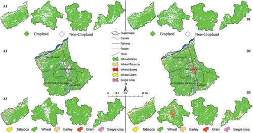
Figure 4 (B1) indicates that croplands extracted from Landsat-8 derived data. Figure 4 (B1) shows Wazirabad, Nowshervirkhan, Kamoke, and Gujranwala sub-districts have a non-cropland area of 19.4%, 7.72%, 12.94%, and 18.92%, and cropland area of 80.6%, 92.28%, 87.06%, and 81.08%, respectively. Landsat-8 derived cropland data had more excellent reliability than the sites with irregular patches. Thus, cropland mapping accuracy was affected mainly by landscape configuration. Figure 4(A1, B1) indicated Landsat-8 data was matched well with cropland of Sentinel-2 data

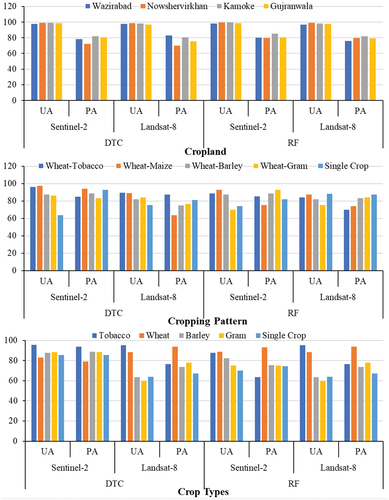
The overall Sentinel-2 derived croplands’ UA and PA Accuracy assessment for Wazirabab was (97.71%, 78.12%), Nowshervirkhan (99.14%, 72.29%), Kamoke (98.98%, 81.85%) and Gujranwala county (98.77%, 80.62%), respectively (Figure 5). Similarly, the UA and PA accuracy result of LANDSAT-8 data were; Wazirabad (97.92%, 82.77%), Nowshervirkhan (98.57%, 69.68%), Kamoke (98.31%, 80.60%), and Gujranwala county (96.72%, 75.40%), respectively (Figure 5).

Figure 5. User accuracy and producer accuracy of cropland, crop types and cropping pattern using DTC and RF when comparing the results of the land cover classification obtained using Sentinel 2 and Landsat 8 satellite images in Gujranwala, Pakistan.

3.1.2. Cropping pattern

The cropping pattern mapping based on multi-temporal remote sensing images described the transition zone between all administrative units (sub-districts) of the study area due to the change of cropping patterns and types. Wheat-Maize has the maximum accuracy with the minimum omission and commission errors. This is realistic because of the temporal profile of the wheat-maize (Figure 3). Single crops have the lowest UA and PA due to a mix of the pixel with other cropping pattern samples.

The spatial dispersal of cropping patterns in Gujranwala for 2021 (Figure 4(A2,B2)) indicate that Wheat-Maize was focused in all sub-district regions except the center Gujranwala district, and Wheat-Gram was scattered primarily in the south and western parts. Wheat-Tobacco and Wheat-Gram mainly were grouped in the southeast and west, and Single crops were distributed during the Gujranwala district. More analysis of the cropping pattern regions shows that Wheat-Maize had the major area in 2021 and had a high PA accounting for 94.29% of the total cropland area. Table 2 represents the cropland area of Wheat-Tobacco, Wheat, Maize, Wheat-Barley, Wheat-Gram, and single cropping pattern derived by Sentinel-2.

Table 2. Area statistics of Sentinel-2 and Landsat-8 derived cropping area using DTC in Gujranwala, Pakistan, in 2021.

	Sentinel-2						Landsat-8
Item	Wheat-Tobacco	Wheat-Maize	Wheat-Barley	Wheat-Gram	Single crop	Total	Wheat-Tobacco	Wheat-Maize	Wheat-Barley	Wheat-Gram	Single crop	Total
Area (km^2)	413.22	1699.22	510.28	98.23	96.06	2817.01	423.55	1730.25	480.22	90.33	92.66	2817.01
Area ratio (%)	14.67	60.32	18.11	3.49	3.41	100	15.04	61.42	17.05	3.21	3.29	100

Using the DTC model, single crops achieved the lowest UA values of 63%, while Wheat–maize had 97%, higher PA due to identifying many cropping pattern pixels using Sentinel-2 data. In the Landsat-8 data, Wheat-tobacco has higher UA, and wheat-maize has more petite PA using the decision tree classification were indicated in Figure 5.

3.1.3. Crop types

The crop type mapping based on multi-temporal remote sensing images describes the transition zone between all administrative units (counties) of the study area due to the change of cropping patterns and types. DTC methods helped identify the crop types using Sentinel-2 and Landsat-8 data in Gujranwala. Sentinel-2 satellite-derived data pinpointed that the adopted method could successfully extract crops. Figure 4 (A3) displays the different crops like tobacco, wheat, barley, gram, and groundnut, indicating that the proposed method can successfully extract crops. Landsat-8 derived data clearly explained in Figure 4 (B3) wheat is the most important crop in all counties in the study area.

Figure 5 shows the UA and PA accuracies for identifying crops using Sentinel-2 data of 2021. Tobacco, the most important crop in the region, has higher user accuracy and producer’s accuracy of 95% and 93%, respectively. In the Landsat-8 data indicated in Figure 5, tobacco has UA (95.34%), while Wheat has higher producer accuracy (93%).

3.2. Classification of RF using Sentinel-2 and Landsat-8 data

3.2.1. Cropland

Sentinel-2/Landsat-8 satellite-derived data were used to extract cropland areas using a random forest model. Sentinel-2 and Landsat-8 are presented in Figure 6(A1, B1). The cropland distribution derived from Sentinel-2 data, as shown in Figure 6 (A1), pinpoints that the croplands are mainly dispersed except the central areas. Wazirabad, Nowshervirkhan, Kamoke, and Gujranwala County have a non-cropland place of 20.3%, 8.48%, 11.93%, and 13.22% and cropland area of 79.7%, 91.52%, 88.97%, and 86.78%, respectively.

Figure 6. Comparison of the spatial extent of cropland, cropping pattern, and crop types using RF method with Sentinel-2 (Left side) and Landsat-8 (Right side) images.

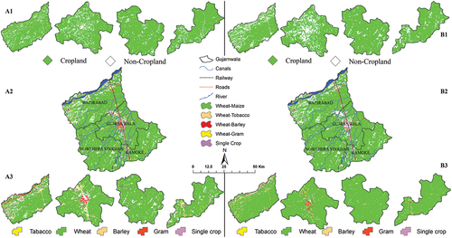
Landsat-8 data indicates the spatial and temporal crop variations in the Gujranwala division. It was indicated that cropland distribution from Landsat-8 data. Figure 6 (A1) pinpointed that the croplands were dispersed mainly in central and south-eastern Gujranwala, Pakistan. Figure 6 (B1) indicated Landsat-8 data. Wazirabad, Nowshervirkhan, Kamoke, and Gujranwala County have a non-cropland area of 20.8%, 8.80%, 11.24%, and 29.18%, and cropland area of 71.2%, 89.20%, 77.76%, and 70.82%, respectively. Nevertheless, misclassification occurred in these areas. For example, in test Kamoke, Wazirabad was misclassified as croplands, while the cropland class was misclassified as other classes.

The overall Sentinel-2 derived croplands’ UA and PA Accuracy assessment for Wazirabab was 98.34% and 80.09%, Nowshervirkhan 99.43% and 79.72%, Kamoke, 99.32% and 85.37%, and Gujranwala 98.57%, and 80.34%, respectively (Figure 5). While for the Landsat-8 derived data, the UA and PA Accuracy assessment was Wazirabad (96.88% and 75.97%), Nowshervirkhan (99.14% and 79.56%), Kamoke (98.31% and 81.88%), and Gujranwala (97.54% and 79.33%), respectively (Figure 5).

3.2.2. Cropping pattern

Each type of cropping pattern has particular traits that manifest itself during the planting, growing, and harvesting stages. This opens up the prospect of utilizing remote sensing time-series data to derive different types of cropping patterns. In point of fact, temporal profile study of crop phenology is crucial when it comes to mapping out crop types. We got maximum accuracy from Wheat-Maize with fewer omission and commission errors. Many spatial dispersals of cropping patterns in Gujranwala in 2021 (Figure 6(A2, B2)) show that Wheat-Maize was mainly focused in all sub-district regions except the center Gujranwala district, and Wheat-Gram was scattered primarily in the south and western parts. Wheat-Tobacco and Wheat-Gram mainly were grouped in the southeast and west, and Single crops were distributed during the Gujranwala district. Moreover, Sentinel-2 and Landsat-8 derived data Wheat-Tobacco, Wheat, Maize, Wheat-Barley, Wheat-Gram, and single cropping pattern have cropland area indicated in Table 3.

Table 3. Area statistics of Sentinel-2 and Landsat-8 derived cropping area using RF in Gujranwala, Pakistan, in 2021.

	Sentinel-2						Landsat-8
Item	Wheat-Tobacco	Wheat-Maize	Wheat-Barley	Wheat-Gram	Single crop	Total	Wheat- Tobacco	Wheat-Maize	Wheat-Barley	Wheat-Gram	Single crop	Total
Area (km^2)	413.22	1699.22	510.28	98.23	96.06	2817.01	423.55	1730.25	480.22	90.33	92.66	2817.01
Area ratio (%)	14.67	60.32	18.11	3.49	3.41	100	15.04	61.42	17.05	3.21	3.29	100

In Sentinel-2 data, all cropping patterns, except wheat-maize, have PA of 75% or higher and UA of 69% or higher. Wheat-Gram has the lowest accuracy with a minuscule commission and omission errors. This is reasonable because the temporal profile of the Wheat-Gram (Figure 3) is considerably different from that of other cropping patterns (Figure 5).

3.2.3. Crop types

In this section, the individual RF algorithms use Sentinel-2 and Landsat-8 data. Then, the traditional and the proposed stacking methods were also implemented. RF method helped identify crop types using Sentinel-2 and Landsat-8 data in Gujranwala. Optical remote sensing data pinpointed that the adopted method could successfully extract crops. Figure 6(A3) displays the different crops like tobacco, wheat, barley, gram, and single crops, indicating that the proposed method can successfully extract crops using Sentinel-2. Landsat-8 derived data clearly explained in Figure 6(B3) wheat is the most important crop in all counties in the study area.

Figure 6 (A3) shows high UA and PA of 88% and 938%, respectively, of wheat cropland derived from Sentinel-2 imagery. Whereas tobacco shows 87% UA, the single crop has UA and PA of 69%, 74% (Figure 5). Figure 5 shows the UA and PA accuracies for identifying crops using Sentinel-2 data of 2021. Wheat, the most important crop in the region, shows the best accuracy with UA of 88% and PA of 93%, higher accuracy than tobacco. Figure 5 represents the Landsat-8 data. Tobacco has higher UA (95%), while Wheat has better PA (93%) than tobacco. Landsat-8 derived crops include wheat, barley, tobacco, gram, and single crop. Tobacco had 95% UA, and 76% PA, respectively, for Landsat-8 derived cropland area (Figure 6 (B3)). UA and PA for Gram achieved the lowest UA of 59%. Most fields’ samples collected from Wheat crops indicated that Wheat is a significant crop and covered a larger area than other crops, as shown in Figure 5.

3.3. Accuracy assessment

Overall accuracy (OA) and kappa coefficient (Kc) Sentinel-2 and Landsat-8 data using DTC and RF classifications were computed and reported according to cropland, cropping pattern, and crop types.

3.3.1. Overall classification

The overall cropland accuracy (OA) evaluation and Kappa (Kc) coefficient result of Sentinel-2 data of Wazirabad were 87.50% and 88.72% of Nowshervirkhan were 63.64% and 93.08%, of Kamoke were 87.50% and 88.72%, and of Gujranwala county are 83.64% and 93.08%, respectively (Table 4). The OA assessment and Kc result of Landsat-8 data of Wazirabad were 82.08% and 78.39%, of Nowshervirkhan are 75.53% and 75.14%, of Kamoke are 82.08% and 75.22%, and of Gujranwala county were 75.53% and 77.84%, respectively (Table 4).

Table 4. Overall accuracy (OA) and kappa coefficient of Sentinel-2 and Landsat-8 data.

Method	Sensor	Parameter	Wazirabad	Nowshervirkhan	Kamoke	Gujranwala
DTC	Sentinel-2	OA	87.50	63.64	87.50	83.64
		Kc	88.72	93.08	88.72	93.08
	Landsat-8	OA	82.08	75.53	82.08	75.53
		Kc	78.39	75.14	75.22	77.84
RF	Sentinel-2	OA	80.09	79.72	98.31	97.54
		Kc	79.94	75.23	96.14	88.23
	Landsat-8	OA	88.72	93.08	85.37	80.34
		Kc	75.97	82.56	81.88	79.33

Sentinel-2 derived cropland OA assessment, and Kc of Wazirabad was 80.09%, and 79.94%, of Nowshervirkhan, were 79.72% and 75.23% of Kamoke are 98.31% and 96.14%, and of Gujranwala county were 97.54% and 88.23%, respectively (Table 4). Landsat-8 derived cropland OA assessment, and Kc of Wazirabad was 88.72%, and 75.97%, of Nowshervirkhan, were 93.08% and 82.56% of Kamoke were 85.37% and 81.88%, and of Gujranwala county were 80.34% and 79.33%, respectively (Table 4).

The overall cropping pattern accuracy (OA) and Kappa coefficient (Kc) were determined using the Sentinel-2 and Landsat-8 data DTC model. Sentinel-2 has 85.06% and 76.38%, and Landsat-8 has 90.79% and 79.02%. Moreover, we identified OA and Kc from the RF model. Sentinel-2 has 92.06% and 83.05%, and Landsat-8 has 92.27% and 88.78%, respectively (Table 5).

Table 5. Overall Accuracy (OA) and Kappa coefficient (Kc) of crop types and cropping pattern using Sentinel-2 and Landsat-8 images.

Methods	Sensor	Crop types		Cropping pattern
		OA (%)	Kc (%)	OA (%)	Kc (%)
DTC	Sentinel-2	97.71	78.12	85.06	76.38
	Landsat-8	98.98	81.85	90.79	79.02
RF	Sentinel-2	97.92	82.77	92.06	83.05
	Landsat-8	98.31	80.60	92.27	88.78

The overall crop type’s accuracy and Kc were determined using the DTC model in the Sentinel-2 and Landsat-8 data. Sentinel-2 has 97% and 78%, and Landsat-8 has 98% and 81%, respectively. Moreover, we identified OA and Kc from the RF model. Sentinel-2 has 97% and 82%, and Landsat-8 has 98% and 80%, respectively (Table 5).

3.4. RF and DTC comparisons using McNemar’s test

We used McNemar’s Chi-squared test to check how the Sentinel-2/Landsat-8 and crop statistical data derived crops at the county level. The differences between the classification outcomes achieved by DTC and RF were assessed using McNemar’s Chi-squared test. The McNemar’s chi-square test results showed that the distribution of crops data, measured through Sentinel-2 derived and Landsat-8 data, is presented in Table 6. It was observed that crops data, measured through different approaches and data, was the same. McNemar’s chi-square test value was significant in each county and crops group. Most of the county’s Sentinel-2 and Landsat-8, and crops-statistical data had two-tailed P values near 1.0%. It means a high correlation between two factors.

Table 6. An overview of the categorization comparisons using McNemar’s Chi-squared test.

Methods	Sensor	Wazirabad		Nowshervirkhan		Kamoke		Gujranwala
		x^2	p	x^2	p	x^2	p	x^2	p
DTC	Sentinel-2	0.50	0.48	1.15	0.40	0.11	0.63	0.10	0.35
	Landsat-8	0.68	0.41	0.73	0.40	0.26	0.63	0.74	0.40
	Crop-statistical	0.03	0.96	0.04	0.85	0.03	0.97	0.02	0.89
RF	Sentinel-2	0.05	0.82	0.01	0.91	0.01	1.00	0.03	0.87
	Landsat-8	0.01	0.91	0.04	0.84	0.03	0.89	0.39	0.55
	Crop-statistical	0.03	0.88	0.10	0.77	0.05	0.97	0.12	0.74

3.5. Comparison of Sentinel-2, Landsat-8, and statistical-based cropland and crop types data

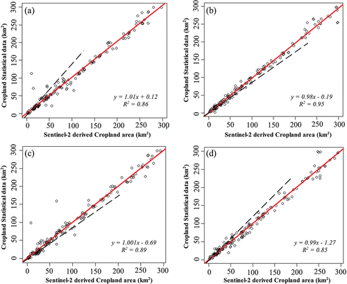
A total of 184 crop samples were used to compare Sentinel-2 and statistical-based cropland of maps. The sites with bigger patch sizes of cropland had higher reliability than the sites with irregular patch sizes, thus, showing that the landscape configuration had a substantial effect on the accuracy of cropland mapping. The adjusted coefficient of determination (R²) at the sub-district level scale in 2021 between crop-statistical and Sentinel-2 derived cropland data was more than 0.86, 0.95, 0.89, and 0.85 as shown in Figure 7(a–d), illustrating this approach’s promise in the progress of Sentinel-2 croplands. Notice that the cropland regression line nearly overlapped at the 1:1 diagonal, further reinforcing the strong arrangement between the estimate of the croplands region and crop-statistical results.

Figure 7. Comparisons of crop-statistical and Sentinel-2 derived data estimation cropland areas for (a) Wazirabad (b) Nowshervirkhan (c) Kamoke (d) Gujranwala.

Correlating the Sentinel-2 derived and crop areas with 2021 statistical data (Table 7) showed high R² values for barley, tobacco, and wheat while low R² for the gram and other crops. It showed that the Sentinel-2 zones for altered categories of crops agreed with corresponding crops-statistical data. The total assessed cropland area encompassed 2817.01 km², which was approximately 118.19 km² higher than the cropland area in national statistics. A great R² value (0.93) and small RRMSE value (0.59) further confirmed that the proposed method could successfully extract cropland area at a large-scale using Sentinel-2 derived data.

Table 7. A real comparison of crop types from Sentinel-2 and crop-statistical data, Gujranwala, in 2021.

Crop type	Sentinel-2-derived estimation (km^2)	Statistical data (km^2)	R^2	RRMSE
Tobacco	408.74	367.95	0.93	56.59
Wheat	2403.42	2326.94	0.90	81.06
Barley	1.99	1.86	0.86	0.26
Gram	2.13	1.42	0.81	1.42
Single crop	0.73	0.65	0.59	0.70
Total	2817.01	2698.82

The relationship between corresponding statistical data and Sentinel-2 derived crop type area (Figure 8(a–d)) shows a conclusion similar to Table 8; tobacco has the most excellent estimation results. The spatial dispersal of crop types in Gujranwala in 2021 (Figure 8(a)) shows that tobacco dispersal is significantly related to cropland dispersal (Figure 7). Wheat seems in the Wheat-Tobacco arrangement, and Wheat-Gram arises at Wheat-Barley and Wheat-Maize forms (Figure 7 (c1)). Analysis of each crop types zone (Table 8) shows that Wheat has the major established zone in Gujranwala, accounting for 85% of the total crop type area, and barley has the least, accounting for only 0.07% total crop-type area.

Figure 8. Areal comparison of crop types from the Sentinel-2 and statistical data of (a) Tobacco; (b) Wheat; (c) Barley: (d) Gram.

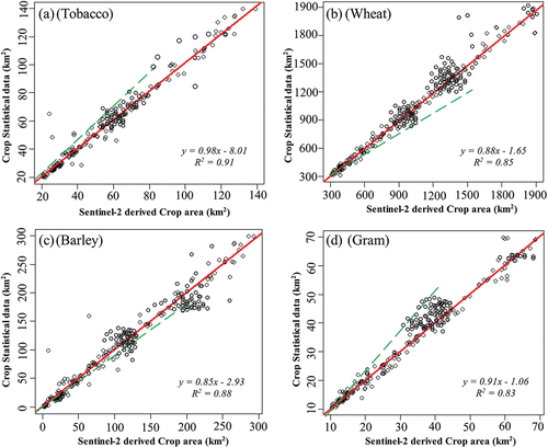
Table 8. A real statistical results of Sentinel-2 derived crop types in 2021 in Gujranwala.

Item	Tobacco	Wheat	Barley	Gram	Single Crop	Total
Area (km^2)	408.74	2403.42	1.99	2.13	0.73	2817.01
Total area of crop type (%)	14.51	85.31	0.07	0.07	0.03	100

4. Discussion

This paper presents the application of a method to map cropland, cropping patterns, and crop types using Sentinel-2 and Landsat 8 time-series data for the period August 2015–December 2021. The different cropping patterns and crop types over the study area were identified using a decision tree classification and Random Forest classification, built based on differences in phenological variables. The Sentinel-2 derived images produced excellent accuracy compared with LANDSAT-8 imagery and official crop statistics for 2020–2021. The wheat-maize cropping pattern is the prevailing cropping pattern in Gujranwala District, Pakistan. This study focused on two cropping patterns that have not been examined in previous studies employing a similar methodology using Sentinel-2 images (Grobler et al. 2012; Ok, Akar, and Gungor 2012).

Croplands and crop patterns have been extracted from typical sample plots using thresholds. However, the thresholds have been subjectively determined, and thus the estimated areas may differ when the criteria are modified. According to the research, the tiny farmland patch sizes (mixed pixels in Sentinel-2 data) led to substantial uncertainty in cropland and crop type area estimates in municipalities with small agricultural areas. Croplands and crop patterns have been extracted from typical sample plots using thresholds. However, the thresholds have been subjectively measured, and thus the estimated areas may differ when the criteria are modified. According to the research, the tiny farmland patch sizes (mixed pixels in Sentinel-2 data) led to substantial uncertainty in cropland and crop type area estimates in municipalities with small agricultural areas. Earlier review (Chen et al. 2016) showed that the pixels’ homogeneity is essential for crop mapping. The impact of mixed pixels may be disregarded in municipalities with huge agricultural fields, but small croplands cannot be ignored in cities with small croplands. The study cannot consider the difficulties in identifying small agricultural areas and the small percentage of maize, single crop, and Wheat in this research. This may lead to an overestimation of Wheat and other double cultivation methods and a bias in assessing crops based on statistics. More research should be done to improve the estimate’s accuracy in regions with small patch sizes.

Several studies have shown how mixed pixels reduce the impact on the mapping accuracy of land covers (Lobell, Cassman, and Field 2009). Spectral mixture analyses have been extensively used in satellite images with medium spatial resolution, such as those from Landsat (Waqas et al. 2021). They have shown to be a productive method for breaking down mixed pixels into fractional objects (Das and Mishra 2017; Kumar and Parikh 2001; Mandal et al. 2020) the difficulty of identifying enough end members using medium spatial resolution images, such as Landsat data. Data fusion techniques may be used to integrate Sentinel-2 and Landsat-8 data to improve the geographical resolution of datasets. However, the enormous amount of data needed across a large area will become an issue. Another approach is to map fractions of agricultural distributions based on Sentinel-2, and Landsat-8 derived cropland data using estimate models (Stroppiana et al. 2012). A regression-based approach to estimating the distribution of fractional croplands is used (Wu et al. 2014).

However, research in the future should focus on developing an approach to estimating fractional areas of different crop types and crop patterns, which would include notable places of small crop patches. It is hard to gather ground-truth data on cropping patterns throughout the state. Most of our crop pattern data were collected in the sub-district of Novshervirkhan during the field research. Because of the importance of crop variability, crop patterns, and crop types may be less precise than in Noshervirkhan in minor crop areas. The established sample-based and Sentinel-2 derived datasets for 2021 were transferred to the 2020 data for cropping pattern maps in Gujranwala when the evaluation was carried out based on statistical information. The results indicated a good match. However, caution should be taken while using the developed technique in different areas of study because of the differences in terrestrial shape and composition of LC. The DTC criteria may need to be adjusted according to the cropping pattern samples in each study (Stroppiana et al. 2012).

The effect of mixed pixels for counties with a large cropland region may be neglected. Still, it can be problematic for counties with smaller cropland areas and have difficulties finding tiny cropland areas and a low areal percentage. Therefore, for those small counties, it is difficult to identify the maize-cotton, cotton-sugarcane, sugarcane-tobacco dual cropping. It can trigger overestimation based on crop statistical data for maize region and other double-cropping systems and distortion in crop form evaluation. A great deal of work has examined strategies for raising the effect of mixed pixels on the quality of land-cover mapping (Lobell, Cassman, and Field 2009; Zhu et al. 2016). Analysis of spectral mixture is proved to be an efficient method for decomposing mixed pixels into fractional artifacts. It is commonly utilized for low spatial resolution image analyses, such as satellite images from Landsat-8 (Liu et al. 2003).

5. Conclusions

Cropland, cropping patterns, and crop type identification and mapping are extremely important for numerous environmental planning and research applications. The collection and creation of data can be made more efficient and dependable through the use of remote sensing. Information gathered from satellites about agriculture can help farmers prepare for the future while also protecting natural resources. Large-scale agricultural operational mapping with great spatiotemporal resolution is now possible.

In this study, Sentinel-2 and Landsat-8 time series served as data input for cropland, cropping-patterns, and crop types mapping using the DTC and RF method. The analysis was applied to optical data in the study area with the same agricultural calendars, parcel morphology, and climatic conditions. Optical remote sensing NDVI time series data were used as input for cropland mapping in this study, with the DTC and RF method used to classify cropland, crop types, and cropping patterns. The research was performed in sub-districts of Gujranwala with the same agricultural calendars, parcel morphology, and climatic conditions. Wheat shows the best accuracy using DTC and Random forest areas as the most important crop. Analysis of each crop type shows that Wheat has the major established zone in Gujranwala, accounting for 85% of the total crop type area, and barley has the least, accounting for only 0.07% total crop-type area.

Our results highlight the Sentinel-2 and Landsat-8 time series value, with crop-statistical data for annual mapping distribution of cropland, cropping-patterns, and crop types with great spatial and thematic detail on a county level. The identification of crop sequence patterns demonstrates the potential of the annual maps in complete crop sequence and future crop rotation analyses on the national scale. Our work identified the temporal changes in cropping patterns and types and a comparative study of the spatial and temporal resolution of medium resolution imagery of the same area. In addition, we show that large-area studies that cover broad environmental gradients are not only important for national reporting but also for illuminating the benefits and drawbacks of using optical and radar data for crop type mapping in a variety of ecological conditions and with a variety of data sources available. This is because the large-area studies are required to reveal the advantages and disadvantages of using optical and radar data.

Acknowledgments

The authors wish to thank the editors and anonymous reviewers for their valuable comments and helpful suggestions. The authors would like to thank Stephen C. McClure for his enthusiastic support and valuable suggestions during the review of the manuscript.

Disclosure statement

The author declares that there is no conflict of interest in this manuscript’s publication. Moreover, the writers have thoroughly addressed ethical issues, including plagiarism, informed consent, fraud, data manufacturing and/or falsification, dual publication and/or submission and redundancy.

Data availability statement

We would like to thank to Sentinel Scientific Data Center of the European Space Agency (ESA) (https://doi.org/10.1080/10095020.2022.2100287) for the Sentinel-2 images and the United States Geological Survey (USGS) (https://doi.org/10.1080/10095020.2022.2100287) for the Landsat 8 images. We are also thankful to the Department of Agriculture & Farmer Welfare, Government of Punjab (https://doi.org/10.1080/10095020.2022.2100287), for providing us the crop statistical data for Gujranwala, Punjab, Pakistan.

Additional information

Notes on contributors

Aqil Tariq

Aqil Tariq received the MS degree in Remote Sensing and GIS from Pir-Mehr Ali Shah Arid Agriculture University, Rawalpindi, Pakistan, in 2016, and PhD degree in photogrammetry and remote sensing from the State Key Laboratory of Information Engineering in Surveying, Mapping and Remote Sensing, Wuhan University, Wuhan, China. Now he is working in the LIESMARS, Wuhan University, China. His research interest areas are 3D Geoinformation, Urban analytics, spatial analysis to examine land use/land cover, Geospatial data science, Urban planning, Crop identification using SAR and Optical Satellite imagery, Agriculture monitoring, Forest Fire, Forest monitoring, forest cover dynamics, spatial statistics, multi-criteria algorithms, Ecosystem sustainability, Hazards risk reduction, Statistical analysis and modeling (Google Earth Engine, HEC-RAS, FlowR, RAMMS, GeoClaw, COSI-Corr, SfM) using Python, R and MATLAB.

Jianguo Yan

Jianguo Yan received his PhD degree from Wuhan University at 2007. He is working as full professor in the State Key Laboratory of Information Engineering in Surveying, Mapping, and Remote Sensing, Wuhan University, Wuhan, China. His current research interests include planetary spacecraft precise orbit determination, planetary gravity field recovery and its interior structure investigation. Recent work are precise orbit determination of MEX and Rosetta, and precise Mars lander positioning with various tracking techniques. The methods we employed are dynamic orbit determination theory, and inversion theory.

Alexandre S. Gagnon

Alexandre S. Gagnon received PhD degree and now he is working in the Biological and Environmental Sciences, James Parsons Building Byrom Street, Liverpool John Moores University. His research interest area are Hydrology, Geography, and Climatology.

Mobushir Riaz Khan

Mobushir Riaz Khan received PhD degree from ITC, University of Twente, Netherland. Now, he is working as professor in School of Agriculture Environment and Veterinary Sciences. His doctoral thesis focused on mapping and monitoring of crop production system using Remote Sensing and GIS along with crop production estimation using crop growth algorithms with remote sensing data. His research interest in geospatial analysis for agriculture, image processing, and environmental monitoring.

Faisal Mumtaz

Faisal Mumtaz received his master’s degree from Aerospace Information Research Institute, Chinese Academy of Sciences, Beijing, China, in 2020. He is now pursuing his Doctoral degree from State key laboratory of remote sensing Science, (AIR-CAS). His main area of expertise is Urban and Infrared Remote Sensing, focusing mainly on Urban Heat Islands (UHI); Urban climate; Urban thermal environmental effects, human settlements; Spatio-temporal analysis, and climate system modeling.

References

- Al-Qaness, M. A. A., A. A. Ewees, H. Fan, A. M. AlRassas, and M. Abd Elaziz. 2022. “Modified Aquila Optimizer for Forecasting Oil Production.” Geo-Spatial Information Science 1–17. online published). doi:10.1080/10095020.2022.2068385.
- Belgiu, M., and O. Csillik. 2018. “Sentinel-2 Cropland Mapping Using Pixel-Based and Object-Based Time-Weighted Dynamic Time Warping Analysis.” Remote Sensing of Environment 204: 509–523. doi:10.1016/j.rse.2017.10.005.
- Belgiu, M., and A. Stein. 2019. “Spatiotemporal Image Fusion in Remote Sensing.” Remote Sensing 11 (7): 818. doi:10.3390/rs11070818.
- Bellón, B., A. Bégué, D. Lo Seen, C. A. De Almeida, and M. Simões. 2017. “A Remote Sensing Approach for Regional-Scale Mapping of Agricultural Land-Use Systems Based on NDVI Time Series.” Remote Sensing 9 (6): 600. doi:10.3390/rs9060600.
- Bradley, J. V. 1968. Distribution-Free Statistical Tests. Hoboken, New Jersey: Prentice-Hall.
- Breiman, L. 2001. “Random Forests.” Machine Learning 45 (1): 5–32. doi:10.1007/978-3-662-56776-0_10.
- Browning, D. M., and M. C. Duniway. 2011. “Digital Soil Mapping in the Absence of Field Training Data: A Case Study Using Terrain Attributes and Semiautomated Soil Signature Derivation to Distinguish Ecological Potential.” Applied and Environmental Soil Science 2011: 421904. doi:10.1155/2011/421904.
- Chander, G., B. L. Markham, and D. L. Helder. 2009. “Summary of Current Radiometric Calibration Coefficients for Landsat MSS, TM, ETM+, and EO-1 ALI Sensors.” Remote Sensing of Environment 113 (5): 893–903. doi:10.1016/j.rse.2009.01.007.
- Chen, Y., X. Song, S. Wang, J. Huang, and L. R. Mansaray. 2016. “Impacts of Spatial Heterogeneity on Crop Area Mapping in Canada Using MODIS Data.” ISPRS Journal of Photogrammetry and Remote Sensing 119: 451–461. doi:https://doi.org/10.1016/j.isprsjprs.2016.07.007.
- Chen, Y., D. Lu, E. Moran, M. Batistella, and L. V. Dutra, I. D. Sanches, R. F. B. da Silva, et al. 2018. “Mapping Croplands, Cropping Patterns, and Crop Types Using MODIS Time-Series Data”. International Journal of Applied Earth Observation and Geoinformation 69: 133–147. doi:https://doi.org/10.1016/j.jag.2018.03.005.
- Chuvieco, E., M. P. Martin, and A. Palacios. 2002. “Assessment of Different Spectral Indices in the Red-Near-Infrared Spectral Domain for Burned Land Discrimination.” International Journal of Remote Sensing 23 (23): 5103–5110. doi:10.1080/01431160210153129.
- Cohen, J. 1960. “A Coefficient of Agreement for Nominal Scales.” Educational and Psychological Measurement 20 (1): 37–46. doi:10.1177/001316446002000104.
- Congalton, R. G. 1991. “A Review of Assessing the Accuracy of Classifications of Remotely Sensed Data.” Remote Sensing of Environment 37 (1): 35–46. doi:10.1016/0034-4257(91)90048-B.
- Das, M. K., and P. Mishra. 2017. “Impacts of Climate Change on Agricultural Yield: Evidence from Odisha, India.” International Journal of African and Asian Studies 38: 58–65.
- Das, P., Z. Zhang, and H. Ren. 2022. “Evaluating the Accuracy of Two Satellite-Based Quantitative Precipitation Estimation Products and Their Application for Meteorological Drought Monitoring Over the Lake Victoria Basin, East Africa.” Geo-Spatial Information Science 1–19. online publiahed. doi:https://doi.org/10.1080/10095020.2022.2054731.
- DeFries, R. S., and J. Townshend. 1994. “NDVI-Derived Land Cover Classifications at a Global Scale.” International Journal of Remote Sensing 15 (17): 3567–3586. doi:10.1080/01431169408954345.
- Dian, R., S. Li, A. Guo, and L. Fang. 2018. “Deep Hyperspectral Image Sharpening.” IEEE Transactions on Neural Networks and Learning Systems 29 (11): 5345–5355. doi:10.1109/TNNLS.2018.2798162.
- FAO. 2017. The State of Food Security and Nutrition in the World. Rome: Building Resilience for Peace and Food Security.
- Gao, F., J. Masek, M. Schwaller, and F. Hall. 2006. “On the Blending of the Landsat and MODIS Surface Reflectance: Predicting Daily Landsat Surface Reflectance.” IEEE Transactions on Geoscience and Remote Sensing 44 (8): 2207–2218. doi:10.1109/TGRS.2006.872081.
- Ghamisi, P., B. Hofle, N. Yokoya, Q. Wang, B. Rasti, N. Yokoya, Q. Wang, et al., 2019. “Multisource and Multitemporal Data Fusion in Remote Sensing: A Comprehensive Review of the State of the Art.” IEEE Geoscience and Remote Sensing Magazine 7 (1): 6–39. doi:10.1109/MGRS.2018.2890023.
- Grobler, T. L., E. R. Ackermann, J. C. Olivier, A. J. van Zyl, and W. Kleynhans. 2012. “Land-Cover Separability Analysis of Modis Time-Series Data Using a Combined Simple Harmonic Oscillator and a Mean Reverting Stochastic Process.” IEEE Journal of Selected Topics in Applied Earth Observations and Remote Sensing 5 (3): 857–866. doi:10.1109/JSTARS.2012.2183118.
- Gu, Y., J. F. Brown, J .P. Verdin, and B. Wardlow. 2007. “A Five‐year Analysis of MODIS NDVI and NDWI for Grassland Drought Assessment Over the Central Great Plains of the United States.” Geophysical Research Letters 34 (6): L06407. doi:10.1029/2006GL029127.
- Gumma, M. K., P. S. Thenkabail, P. G. Teluguntla, A. Oliphant J. Xiong, C. Giri, and V. Pyla. 2020. “Agricultural Cropland Extent and Areas of South Asia Derived Using Landsat Satellite 30-M Time-Series Big-Data Using Random Forest Machine Learning Algorithms on the Google Earth Engine Cloud.” GIScience & Remote Sensing 57 (3): 302–322. doi:https://doi.org/10.1080/15481603.2019.1690780.
- Guru, B., K. Seshan, and S. Bera. 2017. “Frequency Ratio Model for Groundwater Potential Mapping and Its Sustainable Management in Cold Desert, India.” Journal of King Saud University-Science 29 (3): 333–347. doi:10.1016/j.jksus.2016.08.003.
- Hamza, S., I. Khan, L. Lu, H. Liu, F. Burke, S. Nawaz-Ul-Huda, andM.F. Baqa. 2021. “The Relationship Between Neighborhood Characteristics and Homicide in Karachi, Pakistan.” Sustainability 13 (10): 5520. doi:https://doi.org/10.3390/su13105520.
- Han, Y., Y. Wang, and Y. Zhao. 2010. “Estimating Soil Moisture Conditions of the Greater Changbai Mountains by Land Surface Temperature and NDVI.” IEEE Transactions on Geoscience and Remote Sensing 48 (6): 2509–2515. doi:10.1109/TGRS.2010.2040830.
- Hentze, K., F. Thonfeld, and G. Menz. 2016. “Evaluating Crop Area Mapping from MODIS Time-Series as an Assessment Tool for Zimbabwe’s “Fast Track Land Reform Programme”.” PloS One 11 (6): e0156630. doi:10.1371/journal.pone.0156630.
- Hou, H., R. Wang, and Y. Murayama. 2019. “Scenario-Based Modelling for Urban Sustainability Focusing on Changes in Cropland Under Rapid Urbanization: A Case Study of Hangzhou from 1990 to 2035.” The Science of the Total Environment 661: 422–431. doi:10.1016/j.scitotenv.2019.01.208.
- Hussain, S., L. Lu, M. Mubeen, W. Nasim S. Karuppannan, S. Fahad, and A. Tariq. 2022. “Spatiotemporal Variation in Land Use Land Cover in the Response to Local Climate Change Using Multispectral Remote Sensing Data.” Land doi 115:595. doi:https://doi.org/10.3390/land11050595
- Imran, M., I. Basit, M .R. Khan, and S. R. Ahmad. 2018. “Analyzing the Impact of Spatio-Temporal Climate Variations on the Rice Crop Calendar in Pakistan.” International Journal of Agricultural and Biosystems Engineering 12 (6): 177–184. doi:10.5281/zenodo.1317168.
- Imran, M., S. Ahmad, A. Sattar, and A. Tariq. 2022. “Mapping Sequences and Mineral Deposits in Poorly Exposed Lithologies of Inaccessible Regions in Azad Jammu and Kashmir Using SVM with ASTER Satellite Data.” Arabian Journal of Geosciences 15 (6): 538. doi:10.1007/s12517-022-09806-9.
- Isa, S. M., G. P. K. Suharjito, T. W. Cenggoro, and T. W. Cenggoro. 2021. “Supervised Conversion from Landsat-8 Images to Sentinel-2 Images with Deep Learning.” European Journal of Remote Sensing 54 (1): 182–208. doi:10.1080/22797254.2021.1875267.
- Jönsson, P., and L. Eklundh. 2004. “Timesat—a Program for Analyzing Time-Series of Satellite Sensor Data.” Computers & Geosciences 30 (8): 833–845. doi:10.1016/j.cageo.2004.05.006.
- Karnieli, A., N. Agam, R. T. Pinker, M. Anderson, M. L. Imhoff, G.G. Gutman, andN. Panov. 2010. “Use of NDVI and Land Surface Temperature for Drought Assessment: Merits and Limitations.” Journal of Climate 23 (3): 618–633. doi:10.1175/2009JCLI2900.1.
- Kulkarni, N. M. 2017. “Crop Identification Using Unsuperviesd ISODATA and K-Means from Multispectral Remote Sensing Imagery.” International Journal of Engineering Research and Applications 7 (04): 45–49. doi:10.9790/9622-0704014549.
- Kumar, K. K., and J. Parikh. 2001. “Indian Agriculture and Climate Sensitivity.” Global Environmental Change 11 (2): 147–154. doi:https://doi.org/10.1016/S0959-3780(01)00004-8.
- Lambert, M. J., F. Waldner, and P. Defourny. 2016. “Cropland Mapping Over Sahelian and Sudanian Agrosystems: A Knowledge-Based Approach Using PROBA-V Time Series at 100-M.” Remote Sensing 8 (3): 232. doi:10.3390/rs8030232.
- Landerer, F. W., and S. Swenson. 2012. “Accuracy of Scaled GRACE Terrestrial Water Storage Estimates.” Water Resources Research 48 (4): W04531. doi:10.1029/2011WR011453.
- Liaqut, A., I. Younes, R. Sadaf, and H. Zafar. 2019. “Impact of Urbanization Growth on Land Surface Temperature Using Remote Sensing and GIS: A Case Study of Gujranwala City, Punjab, Pakistan.” International Journal of Economic and Environmental Geology 9 (3): 44–49. doi:10.46660/ijeeg.Vol0.Iss0.0.138.
- Liu, Z., T. Sekito, M. Špı́rek, J. Thornton, and R.A. Butow. 2003. “Retrograde Signaling is Regulated by the Dynamic Interaction Between Rtg2p and Mks1p.” Molecular Cell 12 (2): 401–411. doi:10.1016/S1097-2765(03)00285-5.
- Liu, Q., Y. He, H. Li, B. Li, G. Gao, L. Fan, and J. Dai. 2014. “Room-Temperature Ferromagnetism in Transparent Mn-Doped BaSno 3 Epitaxial Films.” Applied Physics Express 7 (3): 033006. doi:10.7567/apex.7.033006.
- Lobell, D.B., K.G. Cassman, and C.B. Field. 2009. “Crop Yield Gaps: Their Importance, Magnitudes, and Causes.” NCESR Publications and Research 34: 179–204. doi:10.1146/annurev.environ.041008.093740.
- Lu, D., and Q. Weng. 2007. “A Survey of Image Classification Methods and Techniques for Improving Classification Performance.” International Journal of Remote Sensing 28 (5): 823–870. doi:10.1080/01431160600746456.
- Ma, L., Y. Liu, X. Zhang, Y. Ye, G. Yin, and B. A. Johnson. 2019. “Deep Learning in Remote Sensing Applications: A Meta-Analysis and Review.” ISPRSs Journal of Photogrammetry and Remote Sensing 152: 166–177. doi:10.1016/j.isprsjprs.2019.04.015.
- Mandal, D., V. Kumar, D. Ratha, J. M. Lopez-Sanchez, A. Bhattacharya, H. McNairn, andY.S. Rao. 2020. “Assessment of Rice Growth Conditions in a Semi-Arid Region of India Using the Generalized Radar Vegetation Index Derived from RADARSAT-2 Polarimetric SAR Data”. Remote Sensing of Environment 237: 111561. doi:https://doi.org/10.1016/j.rse.2019.111561.
- Margono, B.A., S. Turubanova, I. Zhuravleva, P. Potapov, A. Tyukavina, A. Baccini, andS. Goetz. 2012. “Mapping and Monitoring Deforestation and Forest Degradation in Sumatra (Indonesia) Using Landsat Time Series Data Sets from 1990 to 2010.” Environmental Research Letters 7 (3): 034010. doi:https://doi.org/10.1088/1748-9326/7/3/034010.
- Millard, K., and M. Richardson. 2015. “On the Importance of Training Data Sample Selection in Random Forest Image Classification: A Case Study in Peatland Ecosystem Mapping.” Remote Sensing 7 (7): 8489–8515. doi:10.3390/rs70708489.
- Mishra, A. K., and V. P. Singh. 2010. “A Review of Drought Concepts.” Journal of Hydrology 391 (1–2): 202–216. doi:10.1016/j.jhydrol.2010.07.012.
- Mousa, B., H. Shu, M. Freeshah, and A. Tariq. 2020. “A Novel Scheme for Merging Active and Passive Satellite Soil Moisture Retrievals Based on Maximizing the Signal to Noise Ratio.” Remote Sensing 12 (22): 3804. doi doi:10.3390/rs12223804.
- Muller-Wilm, U., J. Louis, R. Richter, F. Gascon, and M. Niezette. 2013. Sentinel-2 Level 2A Prototype Processor: Architecture, Algorithms and First Results. Paper presented at the Proceedings of the 2005 ESA Living Planet Symposium, Edinburgh, UK.
- Naveendrakumar, G., M. Vithanage, H.-H. Kwon, S. Chandrasekara, M. Iqbal, S. Pathmarajah, andW.C.D.K. Fernando. 2019. “South Asian Perspective on Temperature and Rainfall Extremes: A Review”. Atmospheric Research 225: 110–120. doi:https://doi.org/10.1016/j.atmosres.2019.03.021.
- Nicolaou, N., and S. Shane. 2010. “Entrepreneurship and Occupational Choice: Genetic and Environmental Influences.” Journal of Economic Behavior & Organization 76 (1): 3–14. doi:10.1016/j.jebo.2010.02.009.
- Novelli, A., M.A. Aguilar, F.J. Aguilar, A. Nemmaoui, and E. Tarantino. 2017. “AssesSeg—a Command Line Tool to Quantify Image Segmentation Quality: A Test Carried Out in Southern Spain from Satellite Imagery.” Remote Sensing 9 (1): 40. doi:10.3390/rs9010040.
- Ok, A.O., O. Akar, and O. Gungor. 2012. “Evaluation of Random Forest Method for Agricultural Crop Classification.” European Journal of Remote Sensing 45 (1): 421–432. doi doi:10.5721/EuJRS20124535.
- Owojori, A., and H. Xie. 2005. “Landsat Image-Based LULC Changes of San Antonio, Texas Using Advanced Atmospheric Correction and Object-Oriented Image Analysis Approaches”. Paper presented at the 5th international symposium on remote sensing of urban areas, Tempe, AZ.
- Palsson, F., J. R. Sveinsson, and M. O. Ulfarsson. 2017. “Multispectral and Hyperspectral Image Fusion Using a 3-D-Convolutional Neural Network.” IEEE Geoscience and Remote Sensing Letters 14 (5): 639–643. doi:10.1109/LGRS.2017.2668299.
- Pan, Y., X. Li, P. Gong, C. He, P. Shi, and R. Pu. 2003. “An Integrative Classification of Vegetation in China Based on NOAA AVHRR and Vegetation-Climate Indices of the Holdridge Life Zone.” International Journal of Remote Sensing 24 (5): 1009–1027. doi:10.1080/01431160110115816.
- Pandya, M., A. Baxi, M. Potdar, M. Kalubarme, and B. Agarwal. 2013. “Comparison of Various Classification Techniques for Satellite Data.” International Journal of Scientific & Engineering Research 4 (2): 1–6.
- Pelletier, C., S. Valero, J. Inglada, N. Champion, and G. Dedieu. 2016. “Assessing the Robustness of Random Forests to Map Land Cover with High Resolution Satellite Image Time Series Over Large Areas.” Remote Sensing of Environment 187: 156–168. doi:10.1016/j.rse.2016.10.010.
- Petitjean, F., C. Kurtz, N. Passat, and P. Gançarski. 2012. “Spatio-Temporal Reasoning for the Classification of Satellite Image Time Series.” Pattern Recognition Letters 33 (13): 1805–1815. doi:10.1016/j.patrec.2012.06.009.
- Salma, S., S. Rehman, and M. Shah. 2012. “Rainfall Trends in Different Climate Zones of Pakistan.” Pakistan Journal of Meteorology 9 (17): 37–47.
- Samboko, H., I. Abas, W. Luxemburg, H. Savenije, H. Makurira, K. Banda, and H.C. Winsemius. 2020. “Evaluation and Improvement of Remote Sensing-Based Methods for River Flow Management”. Physics and Chemistry of the Earth, Parts A/B/C 117: 102839. doi:https://doi.org/10.1016/j.pce.2020.102839.
- Sanyal, J., and X. X. Lu. 2004. “Application of Remote Sensing in Flood Management with Special Reference to Monsoon Asia: A Review.” Natural Hazards 33 (2): 283–301. doi:10.1023/B:NHAZ.0000037035.65105.95.
- Seelan, S. K., S. Laguette, G. M. Casady, and G. A. Seielstad. 2003. “Remote Sensing Applications for Precision Agriculture: A Learning Community Approach.” Remote Sensing of Environment 88 (1–2): 157–169. doi:10.1016/j.rse.2003.04.007.
- Stroppiana, D., G. Bordogna, P. Carrara, M. Boschetti, L. Boschetti, and P. Brivio. 2012. “A Method for Extracting Burned Areas from Landsat TM/ETM+ Images by Soft Aggregation of Multiple Spectral Indices and a Region Growing Algorithm.” ISPRS Journal of Photogrammetry and Remote Sensing 69: 88–102. doi:10.1016/j.isprsjprs.2012.03.001.
- Tadesse, L., K. Suryabhagavan, G. Sridhar, and G. Legesse. 2017. “Land Use and Land Cover Changes and Soil Erosion in Yezat Watershed, North Western Ethiopia.” International Soil and Water Conservation Research 5 (2): 85–94. doi:10.1016/j.iswcr.2017.05.004.
- Tariq, A., H. Shu, A. Kuriqi, S. Siddiqui, A.S. Gagnon, L. Lu, and N.T.T. Linh. 2021. “Characterization of the 2014 Indus River Flood Using Hydraulic Simulations and Satellite Images.” Remote Sensing 13 (11): 2053. doi:https://doi.org/10.3390/rs13112053.
- Tariq, A., H. Shu, Q. Li, O. Altan, M.R. Khan, M.F. Baqa, and L. Lu. 2021. “Quantitative Analysis of Forest Fires in Southeastern Australia Using Sar Data.” Remote Sensing 13 (12): 2386. doi:https://doi.org/10.3390/rs13122386.
- Thenkabail, P. S., and M. Gamage. 2004. “The Use of Remote Sensing Data for Drought Assessment and Monitoring in Southwest Asia.” IWMI Research Report. 85. ISBN 92-9090-575-1.
- UN. 2015. World economic situation and prospects 2015. doi: 10.1007/BF02929547.
- Waqas, H., L. Lu, A. Tariq, Q. Li, M.F. Baqa, J. Xing, and A. Sajjad. 2021. “Flash Flood Susceptibility Assessment and Zonation Using an Integrating Analytic Hierarchy Process and Frequency Ratio Model for the Chitral District, Khyber Pakhtunkhwa, Pakistan.” Water 13 (12): 1650. doi:https://doi.org/10.3390/w13121650.
- Wu, Z., P.S. Thenkabail, R. Mueller, A. Zakzeski, F. Melton, L. Johnson, and C. Rosevelt. 2014. “Seasonal Cultivated and Fallow Cropland Mapping Using MODIS-Based Automated Cropland Classification Algorithm.” Journal of Applied Remote Sensing 8 (1): 083685. doi:10.1117/1.JRS.8.
- Xu, D., and X. Guo. 2014. “Compare NDVI Extracted from Landsat 8 Imagery with That from Landsat 7 Imagery.” American Journal of Remote Sensing 2 (2): 10–14. doi:10.11648/j.ajrs.20140202.11.
- Yang, J., Y.-Q. Zhao, and J.-C.-W. Chan. 2018. “Hyperspectral and Multispectral Image Fusion via Deep Two-Branches Convolutional Neural Network.” Remote Sensing 10 (5): 800. doi:10.3390/rs10050800.
- Youssef, A. M., H. R. Pourghasemi, Z. S. Pourtaghi, and M. M. Al-Katheeri. 2016. “Landslide Susceptibility Mapping Using Random Forest, Boosted Regression Tree, Classification and Regression Tree, and General Linear Models and Comparison of Their Performance at Wadi Tayyah Basin, Asir Region, Saudi Arabia.” Landslides 13 (5): 839–856. doi:10.1007/s10346-015-0614-1.
- Zhao, H., and X. Chen (2005). Use of Normalized Difference Bareness Index in Quickly Mapping Bare Areas from TM/ETM+. Proceedings. 2005 IEEE International Geoscience and Remote Sensing Symposium, 2005. IGARSS '05, Seoul, Korea, 3, 1666–1668.
- Zhu, Z., S. Piao, R.B. Myneni, M. Huang, Z. Zeng, J.G. Canadell, andP. Ciais. 2016. “Greening of the Earth and Its Drivers.” Nature Climate Change 6 (8): 791–795. doi:https://doi.org/10.1038/nclimate3004.