Estimating optimal substitution scale of urban gasoline taxis by electric taxis in the era of green energy: a case study of Zhengzhou City

ABSTRACT

Electric Taxis (ETs) are the most favored alternatives to Gasoline Taxis (GTs) in cities that aim to reduce environmental pollution. How to develop a reasonable scale on which GTs are substituted by ETs remains a challenge to governments due to the dynamics and complexity of the taxi system. To address this challenge, this paper develops a discrete-event-based simulation framework to simulate participants in the system and estimate the results under different substitution scales, which are helpful to understanding the status changing law of entities under different substitution scales, such as the operating indices of ETs, the unsatisfied travel requirements of passengers, and the usage state of charging facilities. The framework abstracts the behavioral process of ETs into three elements, namely, entity, behavior, and event. The entities are constructed from the information derived from the trajectory data. The behaviors are defined by rules following behavioral logic under anxiety psychology, which is caused by the limited range of ETs. The events are triggered based on rules from reality. With the help of this framework, a multi-objective optimization model is developed to obtain the optimal substitution scale of GTs in the case study area of Zhengzhou City. Overall, the approach could provide a practical tool to address this challenge, which could support further studies of the effect of ETs on urban taxis.

KEYWORDS:

• Electric Taxi (ET)
• substitution scale
• discrete-event simulation
• decision support
• multi-objective optimization

1. Introduction

Urban transportation is facing increasing air pollution and a steadily diminishing supply of fossil fuels (Li et al. 2021b), which leads to increased attention to alternative renewable sources (Kaltschmitt, Streicher, and Wiese 2007; Liu et al. 2021a) and seeking green energy. The electricity of public transport (i.e. taxi, bus) is a critical step for the city government to reduce urban air pollution and decrease the risk of energy dependence on fossil fuels. Therefore, increasing the penetration rate of EVs in public transport is an important effort to achieve green energy. Electric Vehicles (EVs) have been viewed as effective alternatives to GTs (Wang et al. 2015; He et al. 2016; Kong, Ma, and Wang 2016; Shareef, Islam, and Mohamed 2016; Li et al. 2021b) and buses. In urban areas of developing countries like China, the total number of taxis is much higher than buses. It is a particularly important issue to promote ETs in urban areas. Many Chinese cities have implemented ETs aggressively, such as Beijing, Shenzhen, Shanghai, et al. These city governments offer many incentives to encourage taxi drivers to purchase electric vehicles. However, it is still not clear how charging activities affect taxi drivers’ daily operational behaviors, which is of great concern to drivers, especially in cities with under-developed charging infrastructure, like Zhengzhou, Wuhan, Changsha, Hefei, Chongqing, etc., in China. The affections of charging issues are mainly related to the scale of the ET fleet. Also, taxi electrification is challenging and complicated owing to the various influencing factors involved, for example, the acceptance of ETs in the taxi industry, which in turn depends on factors such as the load of power systems, energy consumption, and operation mileage of the ETs (Liang, Correia, and van Arem 2016; Yang et al. 2016; Sun et al. 2017; Tu et al. 2019; Skippon and Chappell 2019). Any reasonable measure on it can bring positive social feedback and further promote taxi electrification (Azadfar, Sreeram, and Harries 2015). In addition, the process could bring a series of social problems, such as weakening the taxi fleet’s ability to satisfy travel demands, reducing the income of drivers, and arousing public complaints regarding government decisions (Liu, and Liu 2016). Therefore, estimating the optimal substitution scale of urban GTs by ETs is still a critical challenge for the scientific decision-making of urban transportation agencies in under-developed cities.

Two categories of methods could be used to determine the number of ETs or EVs that can be accommodated in a city: static mathematical and dynamic simulation methods. In the aspect of static mathematical methods, the direct approach is to predict the future trend according to the historical changing laws of the number of vehicles. For example, the Gompertz model described the growth law of EVs to predict the number of EVs in the next decade (Li, Wang, and Zhang 2014). A supply and demand balance model (Lu and Wang 2004) determined the optimal number of taxis by considering taxi resource utilization. It considers a linear model to describe the relationship between the number of taxis and the influencing factors including mileage, empty-loaded rate, the number of passengers, operating time, and operating speed. In addition, the fluctuating taxi travel demands along with the associated costs (Yang, Wong, and Wong 2002; Liu and Wang 2004) are considered to improve the flexibility of this model. To improve the prediction accuracy limited by linear models, researchers employed a wavelet neural network (Yang, Hua, and Zhang 2012) to approximate the nonlinear relationship between the number of taxis and the influencing factors. Furthermore, a Gray model (Zhang and Liu 2015) was employed to predict the varying trend in the number of taxis, and its prediction error is then employed to train a back propagation (BP) neural network for improving prediction. In short, mathematical models abstract the growth law of the number of taxis into a set of static quantity relations with affecting factors. Future mathematical models could be improved by considering the dynamic and complex mechanism involved in the growth in the number of taxis and EVs (Teodorovic 2003).

Dynamic simulation methods (i.e. Monte Carlo, Multi-Agent Simulation (MAS), network equilibrium, and system dynamics) are promising to determine the number of taxis or EVs because they could consider the operating environment and behavioral characteristics of participants (Brodeur and Nield 2018; Wang et al. 2019), which can be formulated and virtually implemented by computers to estimate the potential and spatiotemporal effects on taxi services. First, the Monte Carlo and Markov chain methods are used to simulate the drive circle of EVs (Wang et al. 2019). For example, Monte Carlo (Hastings 1970) is used to select track pieces that are divided by the TP to form a realistic drive circle, which ensures that the velocity state with high TP is selected at a high probability. The Markov chain method (Gasparini 1997) is used to describe the characteristics of variations in the velocity of EVs through a Transition Probability (TP) matrix approach. Second, the MAS method (Lioris, Cohen, and Arnaud 2009) is used to simulate the taxi operation process under different fleet sizes and to support a detailed analysis in the simulation program. Moreover, MATSim, a commercial traffic simulation platform, is used to simulate the micro behavior of ETs in reality, which uses a dynamic algorithm to match a taxi and a passenger under different electric states (Bischoff and Maciejewski 2014). Since the time and location of vehicles could affect the coming load of the grid, the dynamic simulation methods are widely applied in revealing its spatiotemporal characteristics (Veneri 2017). For example, an adaptive electric vehicle charging model based on MAS (Xydas, Marmaras, and Cipcigan 2016) is proposed to obtain actual electricity demand, generate a pricing strategy for maximizing profits automatically, and simulate the EVs charging decision by rationally responding to new prices. Similarly, an agent-based simulation method (Dallinger and Wietschel 2012) is used to forecast the power price directly and to dynamically adjust the charging behavior of vehicles to reduce the fluctuation of the power grid load. An improved charging mode for EVs based on dynamic simulation (Rao et al. 2015) is introduced to develop induction strategies for different charging scenarios for improving the charging efficiency of EVs. And the scale of hydrogenation stations was investigated based on MAS (Grüger et al. 2018). Third, in the aspect of network equilibrium and system dynamics, a network equilibrium model (Yang and Wong 1998) is proposed to simulate the cruising behavior of taxis in a road network and is used to explore the service performance under different fleet sizes for given equilibrium state parameters. A two-layer model (Wong, Wong, and Yang 2001) was then proposed to improve the previous network equilibrium model by considering traffic congestion and variations in travel demands. Several system dynamics models (Li et al. 2019) were used to simulate and quantitatively evaluate the energy efficiency, carbon emission, and economy of ET systems under different pricing strategies. In addition, reinforcement learning algorithms (Gong et al. 2018) are also used to simulate the dynamic decision-making process of ET, to obtain the charging loads of Charging Stations (CSs) on both temporal and spatial scales. In short, these simulation approaches could generate the travel and charging demands of ETs for determining the number of taxis or EVs according to mathematical probability and the simplified topological structure of road networks. They could be improved by deriving actual demands and spatiotemporal characteristics from the real trajectory data of urban taxicabs in the determination process of the number of taxis or EVs.

The urban taxi electrification is limited to consider in the previous research works due to the application scenario of government, and the existing gap of optimization approaches or tools in considering some complicated factors like real taxi travel demands, facilities of power system, the balance between limited range and income of the ETs. It is still challenging for governments to develop a reasonable scale on which GTs can be substituted by ETs. To address this challenge, the research problem of this paper is to quantify the influence of the electrification scale on the state of the taxi system and further solve the optimal electrification scale of taxis, aiming to provide a basis for the electrification of urban taxis. In this study, there is a basic assumption that the approach to taxi electrification in urban areas is to replace gasoline cars with an equal number of electric cars. This paper proposes an approach by integrating the simulation of the ET’s behaviors with a discrete event-based framework. Within this proposed approach, taxi trajectory data obtained by Global Positioning System (GPS) sensor is used to derive real spatiotemporal demands of taxis such as the starting and ending times of each trip taken in each taxi, time-varying locations of taxis, and distribution of travel demands (Paulista, Peixoto, and Jose 2019). A discrete-event-based simulation framework is introduced to simulate the passenger seeking/servicing/rejecting behavior and Charge Station (CS) searching/queuing behavior through a set of rules following the behavioral characteristics of ETs that differ from GTs (Zhao et al. 2014) while meeting the derived real demands of taxis. Based on this simulation framework, a dynamic simulation process is developed under the constraints of real road networks, the location, and state of Charging Piles (CPs), the running states of ETs, and real spatiotemporal traveling demands of passengers derived from GPS trajectories. Through this simulation process, this study could obtain the quantitative impacts on multiple participants caused by the number of ETs, such as the number of unmet travel requirements of the passengers, electricity consumption of ETs, and usage duration of charging facilities. At last, this study implements a multi-objective optimization model to balance the interests of participants based on the proposed simulation approach. This approach is helpful to determine a reasonable substitution scale for GTs by ETs for supporting the plan of taxi electrification by urban transportation agencies. Besides this, it could also provide a practical tool to support further studies on the ET market or intelligent transportation systems as well as the influence of ET on urban taxis or public transportation services.

The remainder of this paper is structured as follows: Section 2 introduces the proposed methodology including the simulation framework and system elements; Section 3 introduces the experimental design and simulation result analysis under different scenarios; Section 4 presents a multi-objective optimization model to optimize the number of ETs constrained by current electricity facilities. The conclusions of the study are drawn in Section 5.

2. The proposed approach

To estimate the optimal substitution scale of urban GTs by ETs, this study proposes an integrated approach, which consists of three steps, namely, i) deriving the real travel demands from taxi GPS trajectories (Keler, Krisp, and Ding 2019), ii) designing a discrete-event-based simulation framework to simulate (ET, passenger and charging facility) entities (operational and charging), behaviors and (passenger waiting, Origin-Destination (OD) accepting/rejecting, charging and waiting for charging) events, iii) solving the optimization problem of estimating optimal substitution scale with multi-objectives, for example, consumed power, waiting-time of charging, load pressure of charging facilities, the average daily income of ET.

The first step is to derive the real travel demands from taxi GPS trajectories. The starting and ending time of trajectory data collection is 00:00:00 to 23:59:59 on 1 July 2018. The data involves 8650 taxis, with a total of 6,814,976 track point records. Each taxi GPS trajectory is defined as a series of GPS points with attributes (vehicle ID, timestamp, longitude, latitude, speed, direction, and service state) (see Table 1). The service state is no service (0) or in service (1). The GPS trajectory point with changing service state from 0 to 1 is viewed as the start point of a trip serviced by this taxi. The following series of GPS trajectory points with changing state from 1 to 0 is viewed as the end point of this trip. As a result, the GPS trajectory point pair {start point, end point} is an actual passenger trip serviced by the taxi. All taxi trajectories are filtered by this step to derive all traveled trips by taxi passengers. The second and third steps are critical ones in the proposed approach, which will be described in the following subsections.

Table 1. An example of taxi GPS trajectory for identifying serviced trips by taxi.

Vehicle ID	Timestamp	Longitude	Latitude	Speed	Direction	Service state	Trip
822022731	2018/7/1 9:59	113.XXXX	34. XXXX	48	0
822022731	2018/7/1 10:00	113.XXXX	34. XXXX	16	84	1	Start point
…	…	…	…	…	…	1
822022731	2018/7/1 10:35	113.XXXX	34. XXXX	22	356	1	End point
822022731	2018/7/1 10:36	113.XXXX	34. XXXX	28	356	0

2.1. Simulating the ET’s behaviors using a discrete event-based framework

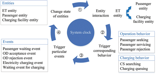
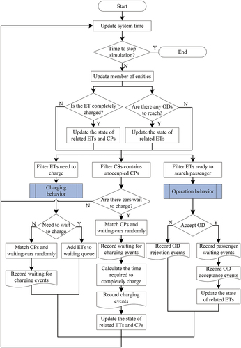
The ET system could be viewed as discrete for its state changes at discrete points in time. Discrete event-based simulation (Paulista, Peixoto, and Jose 2019) is a computational modeling approach, which is suitable to simulate the dynamic evolution of the ET system in a sequence of discrete points. The evolution of the ET system is based on a logic loop as shown in Figure 1. The loop revolves around three system elements (entities, behaviors, and events) and consists of four steps, namely, modeling interactions between entities, triggering behaviors related to interactions, triggering events according to behavior, and changing the state of entities after events.

Figure 1. The logic of ET simulation.

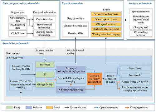
The proposed simulation framework based on the logic loop is given in Figure 2. This framework comprises four modules, namely data pre-processing, simulation, record, and analysis. The data pre-process module derives the information of taxis, travel demands, and charging facilities from raw taxi trajectory data and Point Of Interest (POI) data, which would be used in the simulation module. The simulation module, the core part of this framework, contains the special behavioral mechanism caused by ETs’ characteristics such as range anxiety. The record module is used to record the necessary information when events occur. It also reclaims ETs after finishing the simulation and recycles unmet ODs that have not been served after a long wait. The analysis module supports the statistics of ETs including operation indices (i.e. income and mileage utilization), the service level to travel demands, the charging pressure of charging facilities, and the cost for ETs to find a CS.

Figure 2. Simulation framework of ETs’ behavior.

Within the proposed framework, a time synchronization mechanism called Double Clock (DC) is used to establish the time order among all the participants. The DC refers to the System Clock (SC) and Individual Clock (IC). The SC serves as the unique time reference in the simulation. The IC exists in each entity, which is responsible for recording the end time of the continuous activities. Thus, IC is always ahead of SC. For example, for an ET, IC records the end time of charging or carrying passengers, and the ET will be locked until SC is pushed to IC to avoid access conflict by other entities.

The following subsections introduce the details of the simulation module: i) constructions of entities, ii) interactions between entities and corresponding behaviors, iii) triggering events according to behaviors, iv) changing the state of entities by events in the framework.

2.1.1. Entities

Definition 1.

An ET entity corresponds to an ET in the real world, which contains ET’s necessary attributes. An ET entity is defined as:

(1) $E_{ET}=\left\{VID,T_s,T_e,L_{ET},T_{ind}^{ET},S_{oc}^{ET},SOC,V_s^{ET},M_{rem}\right\}$(1)

where $VID$ is the unique ID of the ET. $T_s$ and $T_e$ refer to the time points when the ET enters and leaves the simulation program, respectively. $L_{ET}$ is the location of the ET (i.e. latitude and longitude). $T_{ind}^{ET}$ is the individual clock for the ET. $S_{oc}^{taxi}$ means the occupancy or service state of the ET (0 or 1). $SOC$ refers to the remaining capacity of the battery. $V_s^{ET}$ represents the current speed of the ET. $M_{rem}$ is the remaining millage with $SOC$.

Definition 2.

A passenger entity corresponds to an OD derived from taxi GPS trajectory. The entity is devised as follows:

(2) $E_{OD}=\left\{ODID,L_s^{OD},L_e^{OD},C_{mil}^{OD},C_t^{OD},C_m^{OD},T_{gen},T_{dis}\right\}$(2)

where $ODID$ is the unique ID of the OD.$L_s^{OD}$ and$\hspace{0.17em}{L}_e^{OD}$ are the locations of the origin and destination. $C_{mil}^{OD}\hspace{0.17em}$and $C_t^{OD}$record the mileage and time cost of the OD. $C_m^{OD}$ is the money that the passenger pays for the OD. $T_{gen}$ and $T_{dis}$ are the time points when the OD generates and disappears. $T_{dis}$ is calculated by $T_{gen}$ plus $T_{{\epsilon }_w}$. Here $T_{{\epsilon }_w}$ is the waiting time length of passengers, which should be reflected in simulation because passengers wait for taxis within limited patience. In this study, $T_{{\epsilon }_w}$ is set to 12 min according to the study (Zhao et al. 2014). If an OD is not served by an ET after $T_{dis}$, then it is regarded as unmet and gets removed from the simulation program by the record module.

Definition 3.

Charging facility entities correspond to CS and its CPs. A CS is equipped with more than one CP. Here, CS and CP entities are formulated as follows:

(3) $E_{cs}=\left\{CSID,L_{cs}\right\}$(3)

(4) $E_{cp}=\left\{CSID,CPID,T_{ind}^{cp},S_{occ}^{cp},P\right\}$(4)

where $CSID$ is the unique ID of a CS to link with its CPs. $L_{cs}$ is the location of the CS entity, which is shared by all CPs within it. $T_{ind}^{cp}$ is the individual clock of a CP, usage state $S_{occ}^{cp}$= {0, 1} (0 means the CP is idle, and 1 means the CP is in service). $P$ is the electric power of the CP.

2.1.2. Interactions between entities and corresponding behaviors

ETs interact with service facilities and public transportation in both the virtual space and physical spaces (Wu, Gui, and Yang 2020). In the simulating process, interactions are always initiated by ETs, and they occur in two scenarios. One is in the operating process, ETs in service interact with ODs and decide whether to serve them or not by forecasting the $SOC$ after arriving at the $\hspace{0.17em}{L}_e^{OD}$. The other interaction occurs when ETs need to be recharged. These ETs interact with CPs to obtain the $S_{occ}^{cp}$ and the distance to the CSs, and this information helps decide which CS to choose.

In the operating process, there are OD seeking, serving, and rejecting behaviors could be triggered. Seeking behavior is implemented by choosing a strategy to find an OD, and after that, the serving/rejecting behavior is triggered to serve the OD or not.

Definition 4.

OD-seeking behavior refers to strategies adopted by ETs to find ODs and get divided into moving and waiting in this study. Drivers adopting the moving strategy will go to the nearest$L_s^{OD}$ of the OD, while drivers adopting the waiting strategy will stay in places. Which strategy to take depends on the decision process as follows: First, supposing the current system clock is $T_{sys}$, the simulation module selects ODs generated before $T_{sys}$ and not gotten serviced yet (Equation (5)(5) $T_{gen}<T_{sys}<T_{dis}$(5) ). Second, the path distance between ETs and ODs will be calculated using the Dijkstra algorithm constrained by the road network, to select the nearest OD for each ET (Equation (6)(6) $MinDis=\mathrm{M}\mathrm{i}\mathrm{n}\left\{\mathrm{d}\mathrm{i}\mathrm{s}\mathrm{t}\mathrm{a}\mathrm{n}\mathrm{c}\mathrm{e}\left(L_{ET},L_s^{OD}\right)\right\}$(6) ). Furthermore, the time cost to the nearest OD will be estimated according to the speed of the ET (Equation (7)(7) $T_{move}=\frac{MinDis}{V_s^{ET}}$(7) ). If the time cost is so long that the OD will disappear after the ET arrives, it will be viewed as the ODs near the ET are sparse, which would result in a low success rate for the moving strategy. Thus, the waiting strategy then gets adopted to save electricity. If the ET can arrive before the $T_{dis}$ and the travel cost $M_{cost}$ (km) is less than the acceptable distance $MaxDis$ of the ET (km) extracted from trajectory data, the moving strategy will be adopted according to Equation (9)(9) $Strategy=\left\{\begin{array}{cc}moving,& T_{arrival}\le T_{disappear}and{M}_{cost}\le MinDis\\ waiting,& otherwise\end{array}\right.$(9) .

(5) $T_{gen}<T_{sys}<T_{dis}$(5)

(6) $MinDis=\mathrm{M}\mathrm{i}\mathrm{n}\left\{\mathrm{d}\mathrm{i}\mathrm{s}\mathrm{t}\mathrm{a}\mathrm{n}\mathrm{c}\mathrm{e}\left(L_{ET},L_s^{OD}\right)\right\}$(6)

(7) $T_{move}=\frac{MinDis}{V_s^{ET}}$(7)

(8) $T_{arrival}=T_{ind}^{ET}+T_{move}$(8)

(9) $Strategy=\left\{\begin{array}{cc}moving,& T_{arrival}\le T_{disappear}and{M}_{cost}\le MinDis\\ waiting,& otherwise\end{array}\right.$(9)

where $T_{move}$ is the time cost of moving, $distance\left(L_{ET},L_s^{OD}\right)$represents the path distance between the locations of ETs and ODs, $T_{arrival}$ is the expected arrival time of the ET to the nearest $L_s^{OD}$ of the OD.

Definition 5.

OD choosing behavior (OD serving/rejecting) refers to serving the OD or rejecting it. Generally, rejecting ODs is illegal for GTs, but it is common among ETs. According to the survey of ET owners, 80% of them stated the experience of rejecting ODs (SMN 2018). And the main reason for this is the anxiety about $SOC$ (Noel et al. 2019), it happens when the remaining $SOC$ is lower than a psychological threshold. Moreover, the distance to the nearest CS of the $\hspace{0.17em}{L}_e^{OD}$also affects whether to serve the OD or not when the ET is in a low $SOC$. In the paper (Tian et al. 2014), it is demonstrated that the last OD accepted before the ET is charged is always near a CS, and drivers reject ODs that are inconvenient for recharging when the $SOC$ is low. Rejecting ODs would prolong the waiting time of passengers and lead to higher cost and lower operating efficiency of ETs, thus it should be reflected in the simulation.

Therefore, the simulation rules of OD choosing behavior consider the anxiety about $SOC$ and the charging convenience around $\hspace{0.17em}{L}_e^{OD}$of ODs. Firstly, the degree of driver’s anxiety is divided into three levels based on $SOC$, namely, no anxiety, anxiety, and risky to shut down. To set the $SOC$ break points of these levels, it is realized that the $SOC$ of ETs is evenly distributed between 30% and 50% before charging (Bi et al. 2017). This demonstrates that drivers do not consider charging when the $SOC$ is above 50% because they have no anxiety; however, they generally charge the ETs before the $SOC$ is below 30% because this would be risky to shut down. Therefore, the anxiety levels of drivers are summarized in Table 2. For the first level, drivers choose ODs without considering the charging problems. For the second level, drivers select ODs prudently considering $SOC$. For the last level, drivers solely consider the charging problem and no longer serve ODs.

Table 2. Anxiety scale of the driver.

The degree of driver’s anxiety	$SOC$
No anxiety	>50% (Bi et al. 2017)
Anxiety	30%~50% (Bi et al. 2017)
Risky to shutdown	<30% (Bi et al. 2017)

The flow of ETs’ behavior in the operating process including OD seeking and choosing behavior is shown in Figure 3. When choosing an appropriate OD for an ET, the first to consider is whether the distance of the OD is beyond the max acceptable distance $MaxDis$ of the ET. If so, the ET rejects the OD; otherwise, the continuing judgments are executed: If it is estimated that $SOC$ >50% after reaching$\hspace{0.17em}{L}_e^{OD}$ of the OD, it would not cause anxiety, and the ET accepts the allocated OD. If the distance of the OD is extremely long resulting that the ET would be risky to get out of service ($SOC<30\mathrm{\%}$) after finishing the service, the driver then refuses the OD. If $30\mathrm{\%}<SOC<50\mathrm{\%}$, the driver will further evaluate the charging convenience $\hspace{0.17em}{L}_e^{OD}$ of the OD. If $SOC$ after the service is sufficient enough to move from $\hspace{0.17em}{L}_e^{OD}$ of the OD to the nearest CS, the driver will accept the OD; otherwise, he/she will refuse it.

Figure 3. Simulation flow chart of ETs’ operational behavior.

When ETs need to charge, the CP searching and CS seeking behaviors could be triggered. The former aims to find an idle CP for the ET. If it fails, the latter would be triggered to choose an appropriate CS for the ET to wait in queue. The following part defines these behaviors individually.

Definition 6.

CP searching behavior refers to the process that ETs search for idle CPs. In simulation, these ETs are able to get the location of the nearest CS with idle CPs, which is already realized in the real world. If the CS is too far to reach before the $SOC$ falls to 30%, the CS-seeking behavior then be triggered.

Definition 7.

CS seeking is defined as the process of choosing an appropriate CS for the ET, within which the waiting time length is considered. ETs go to the nearest CS first, if there are already several ETs in the line at the CS, the driver would make a comparison between the number of queuing cars ($N_{qc}$) and CPs ($N_{cp}$). If $N_{qc}<N_{cp}$, the waiting time for the ET in the current CS will not exceed the charging time of one car, the ET would choose the CS. Otherwise, the ET would go to the next CS nearly, which would be repeated until an appropriate CS is found or the $SOC$ of the ET is not sufficient to reach the next CS. The flow of behaviors above is shown in Figure 4.

Figure 4. Simulation flow chart of CS searching behavior.

2.1.3. Events triggered by behaviors

Events would be triggered by specific behaviors to change states of relevant entities. There are 5 events considered in this framework, namely, passenger waiting, OD accepting, OD rejecting, charging, and waiting for charging events. These events are described in detail below.

Definition 8.

The passenger waiting event is triggered when an OD is served by an ET or is reclaimed by the record module after the system time is beyond $T_{dis}$. Meanwhile, the necessary information about the event would be recorded as Equation (10)(10) $Even{t}_{P\mathrm{\_}Wait}=\{ODID,t_{wait}^p\}$(10) :

(10) $Even{t}_{P\mathrm{\_}Wait}=\{ODID,t_{wait}^p\}$(10)

(11) $t_{wait}^p=T_{sys}-T_{gen}$(11)

Where $t_{wait}^p$ is the time cost of passenger waiting calculated by Equation (11), and the $T_{sys}$ refers to the system time when the event occurs.

Definition 9.

The OD accepting event is defined as that an ET serves an OD. This occurs simultaneously with the passenger waiting event. The attributes of the event as Equation (12)(12) $Even{t}_{OD\mathrm{\_}accept}=\{VID,ODID,T_s^{OD},T_e^{OD}\}$(12) shows.

(12) $Even{t}_{OD\mathrm{\_}accept}=\{VID,ODID,T_s^{OD},T_e^{OD}\}$(12)

where $T_s^{OD}$ is the system time when the event occurs, and the $T_e^{OD}$ is the end time obtained by forecasting through Equation (13)(13) $T_e^{OD}=T_s^{OD}+\frac{C_{mil}^{OD}}{V_s^{ET}}$(13) . $C_{mil}^{OD}/V_s^{ET}$ refers to the duration of the OD allocated to the ET.

(13) $T_e^{OD}=T_s^{OD}+\frac{C_{mil}^{OD}}{V_s^{ET}}$(13)

Definition 10.

The OD rejecting event is the opposite of the OD accepting event. Both of them are results of OD choosing behavior. And this event is triggered when the ET considers the OD is not appropriate to serve and is formed as Equation (14)(14) $Even{t}_{OD\mathrm{\_}reject}=\{VID,ODID,M_{rem}\}$(14) .

(14) $Even{t}_{OD\mathrm{\_}reject}=\{VID,ODID,M_{rem}\}$(14)

Definition 11.

The charging event is defined as the process that ET accesses the power grid to charge. The attributes are as shown below:

(15) $Even{t}_{charge}=\{CPID,VID,T_s^{charge},t_{charge}\}$(15)

where the $T_s^{charge}$ is the system time when the ET accesses the CP. The $t_{charge}$ is the time cost for charging and is estimated by Equation (16)(16) $t_{charge}=\left(kM-M_{rem}\right)\times \frac{Q_{100}}{100P}$(16) where the charging process is considered as a linear process:

(16) $t_{charge}=\left(kM-M_{rem}\right)\times \frac{Q_{100}}{100P}$(16)

where $k$ denotes the adjustment coefficient of the target $SOC$ for charging. $M$ is the driving range under full power; $Q_{100}$ is the power consumption of 100 km, which is 19.5 kW·h in (Autotimes 2016). As most ET batteries are lithium batteries, it is conducive to extending the battery life by charging and discharging between 25% and 75% (Meng et al. 2016), so this study considers 75% of the battery capacity as the charging target $SOC$, meaning that $k$ = 0.75.

Definition 12. The waiting event for charging is defined as the whole process of ET from joining in a waiting queue to recharging. The event is formed as below:

(17) $Even{t}_{Wait\mathrm{\_}for\mathrm{\_}charg}=\left\{CSID,VID,T_s^{queue},T_e^{queue},N\right\}$(17)

Where $T_s^{queue}$ is the system time when the ET joins in the waiting queue of the CS and $T_e^{queue}$ is the time when the ET begins to recharge. $N$ records the CS searching times before the ET joins the waiting queue in the CS.

2.1.4. Changing the status of entities after events

When an OD is accepted by an ET, the passenger waiting event gets triggered, and the served OD would be removed from the OD list. Simultaneously, the serving event occurs, and the status of ET is updated as follows: the $S_{oc}^{ET}$ switches to 1, and the $M_{rem}$ is reduced by subtracting the Distance of the OD, besides, the $L_{ET}$ is updated as the $L_e^{OD}$ of the OD, and the $T_{ind}^{ET}$ would be pushed forward to the $T_{end}^{OD}$. The $\mathrm{S}\mathrm{p}\mathrm{e}\mathrm{e}\mathrm{d}$ is updated by the average speed of the OD, which is derived from the GPS data and able to reflect the actual traffic condition at that time.

(18) $S_{oc}^{ET}=1$(18)

(19) $M_{rem}=M_{rem}-C_{mil}^{OD}$(19)

(20) $L_s^{OD}=L_e^{OD}$(20)

(21) $T_e^{OD}=T_s^{OD}+t_{cost}$(21)

(22) $T_{ind}^{ET}=T_e^{OD}$(22)

(23) $V_s^{ET}=\frac{C_{mil}^{OD}}{t_{cost}}$(23)

When an OD is rejected by an ET, the rejecting event then gets triggered, and the ET would seek for another passenger at next system time, and the $T_{ind}^{ET}$ is updated as Equation (24)(24) $T_{ind}^{ET}=T_{sys}+1$(24) shows to ensure the ET would be called next time.

(24) $T_{ind}^{ET}=T_{sys}+1$(24)

When an available CP is assigned to the ET, the charging event would be triggered. Both the ET and CP are locked until the charging ends, the $S_{oc}^{ET}$ switches to 1, the $T_{ind}^{ET}$ and $T_{ind}^{cp}$ are pushed forward to the end of the charging, and the $M_{rem}$ is updated as pre-set value.

(25) $S_{occ}^{cp}=1$(25)

(26) $T_{ind}^{ET}=T_{ind}^{cp}=T_{sys}+t_{charge}$(26)

(27) $M_{rem}=kM$(27)

When an appropriate CS is found for the ET to join in the waiting line, the waiting event for charging would be triggered and make the ET get registered in the waiting queue of the chosen CS.

The whole simulation flow is depicted in Figure 5. The specific steps are described as follows:

Figure 5. Simulation flow diagram.

1. When the simulation starts, the elements including the road network, system clock, and all entities are first initialized.

2. It is determined whether to terminate the simulation.

3. The members of ET and passenger entities are updated. The external entities activated by the $T_{sys}$ will join in the simulation from the pre-processing module. The internal entities that have completed the simulation are reclaimed by the record module.

4. The status of the entities is updated. If it is time for some ETs to finish the serving of passengers, then these ETs are unlocked ($S_{occ}^{ET}=0).$If it is time for some other ETs to complete the charging process, then $S_{occ}^{cp}$ is changed to be available. And the ETs are unlocked and their $SOC$ is updated.

5. Vacant ETs with sufficient $SOC$ would trigger operational behaviors to serve passengers. As a result, the OD accepting or rejecting event is triggered. Once vacant ETs remain low $SOC$, they have to trigger charging behaviors to replenish electricity. The charging or waiting event occurs depending on the available CPs. As for ETs that have been waiting in line at a CS, the CS would identify if there are any CPs to be released. All ETs are sorted by their waiting start time in ascending order. They are matched to the available CPs according to the first-in-first-out rule. At the same time, the charging events are triggered. As for the ET seeking for a CP, if there are available idle CPs, the ET then goes charging directly and the charging event then happens; otherwise, the ET would search for an appropriate CS to wait in line and the waiting event then occurs.

6. All the events that occurred in step 5 should be recorded.

7. The system clock is updated and the process returns to step 2.

2.2. Optimizing the substitution scale with multi-objectives conditions

It is a multi-objective optimization problem to optimize the substitution scale of urban GTs by ETs. By considering the ETs’ mission of saving energy, the function as public transport, and the greatest concerned charging issue, the optimal objectives are set up to maximize saved gasoline $Q_T$ by ET fleet, maximize its service level $S_{ET}$, and minimize the waiting duration for charging $T_{wait}$ (Equation (28)(28) $L_{obj}\left(N_{ET}\right)=\left\{Q_T\left(N_{ET}\right),S_{ET}\left(N_{ET}\right),-T_{wait}\left(N_{ET}\right)\right\}$(28) ). In addition, the revenue of ETs’ $R_{ET}$ should be about the same as GTs’ $R_{gasoline}$, which is considered as the constraint condition.

Maximize:

(28) $L_{obj}\left(N_{ET}\right)=\left\{Q_T\left(N_{ET}\right),S_{ET}\left(N_{ET}\right),-T_{wait}\left(N_{ET}\right)\right\}$(28)

Subject to:

(29) $R_{ET}\left(N_{ET}\right)\ge R_{gasoline}$(29)

(30) $Q_T\left(N_{ET}\right)=N_{ET}\ast q_{gasoline\mathrm{\_}avg}$(30)

(31) $q_{gasoline\mathrm{\_}avg}=q_{100}\ast \frac{M}{100}$(31)

(32) $S_{ET}\left(N_{ET}\right)=\left\{\begin{array}{c}1,N_{ET}<N_{bp1}\\ \alpha ln\left(N_{ET}\right)+\beta ,N_{bp1}\le N_{ET}<N_{bp2}\\ k{N}_{ET}+b,N_{ET}\ge N_{bp2}\end{array}\right.$(32)

(33) $T_{wait}\left(N_{ET}\right)=\left\{\begin{array}{c}\mu {N_{ET}}^{\sigma },N_{ET}<N_{bp3}\\ a_0{N_{ET}}^2+b_0{N}_{ET}+c_{0,}{N}_{ET}\ge N_{bp3}\end{array}\right.$(33)

(34) $R_{ET}=\left\{\begin{array}{c}{a}_1{N_{ET}}^2+b_1{N}_{ET}+c_1,N_{ET}\le N_{bp2}\\ k_1{N}_{ET}+b_2,N_{ET}>N_{bp2}\end{array}\right.$(34)

(35) $r_{ET}=Incom{e}_{ET}-Cos{t}_{ET}$(35)

(36) $Incom{e}_{ET}=\left\{\begin{array}{c}{i}_0,M_{ET}\le M_0\\ i_0+\left(M_{ET}-M_0\right)\ast i_1,M_{ET}>M_0\end{array}\right.$(36)

(37) $Cos{t}_{ET}=\frac{M_{ET}}{100}\ast e_{100}\ast Pric{e}_e$(37)

where $Q_T$ is the total amount of gasoline that should be consumed without substitution, which is calculated as Equation (30)(30) $Q_T\left(N_{ET}\right)=N_{ET}\ast q_{gasoline\mathrm{\_}avg}$(30) , $N_{ET}$is the substitution scale. The $q_{gasoline\mathrm{\_}avg}$ is the gasoline consumption of a GT calculated by the product of fuel consumption per 100 km $q_{100}$ and daily driving range $M.$ Refer to BYD F3, a common type of GT, $q_{100}$ is set as 5.9 L/100 km. M is set as 257 km according to statistics of its operating data. $S_{ET}$ is defined as the rate of served travel demands by ETs and GTs under the same fleet size (Equation (32)(32) $S_{ET}\left(N_{ET}\right)=\left\{\begin{array}{c}1,N_{ET}<N_{bp1}\\ \alpha ln\left(N_{ET}\right)+\beta ,N_{bp1}\le N_{ET}<N_{bp2}\\ k{N}_{ET}+b,N_{ET}\ge N_{bp2}\end{array}\right.$(32) ). $T_{wait}$ is the total waiting duration of ET fleet in a day, which reflects the service pressure of charging facilities (Equation (33)(33) $T_{wait}\left(N_{ET}\right)=\left\{\begin{array}{c}\mu {N_{ET}}^{\sigma },N_{ET}<N_{bp3}\\ a_0{N_{ET}}^2+b_0{N}_{ET}+c_{0,}{N}_{ET}\ge N_{bp3}\end{array}\right.$(33) ). $R_{ET}$ (Equation (34))(34) $R_{ET}=\left\{\begin{array}{c}{a}_1{N_{ET}}^2+b_1{N}_{ET}+c_1,N_{ET}\le N_{bp2}\\ k_1{N}_{ET}+b_2,N_{ET}>N_{bp2}\end{array}\right.$(34) is a function of $N_{ET}$describing the relationship between the average profit of ETs $r_{ET}$ (Equation (35))(35) $r_{ET}=Incom{e}_{ET}-Cos{t}_{ET}$(35) and the ET fleet size.

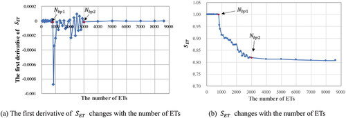
The changing regulation of $S_{ET}$ with $N_{ET}$ is shown in Figure 6. In Figure 6(b), as $N_{ET}$ increases, the competition on travel demands gets more intense, and $S_{ET}$ declines. There appear two break points because of the charging issue. Before the first break point $N_{bp1}$, $N_{ET}$ is relatively small and the charging demands could be met well, so that the operation process is almost unaffected and $S_{ET}$ maintains a high level. After $N_{bp1}$, some ETs that need to be recharged must wait for idle CPs, which causes $S_{ET}$ declines until the system is saturated at the second break point $P_{bp2}$. When $N_{ET}\ge N_{bp2}$, the system is saturated and $S_{ET}$ stays at a low level. The piecewise regression function between $S_{ET}$ and $N_{ET}$ is shown as Equation (32) where $N_{bp1},N_{bp2},\alpha ,\beta ,k,b$ are undetermined parameters. By the first derivative of $S_{ET}$, $N_{bp1}\mathrm{a}\mathrm{n}\mathrm{d}{N}_{bp2}$ are obvious to find (see Figure 6(a)).

Figure 6. The changing regulation of $S_{ET}$ under different fleet sizes.

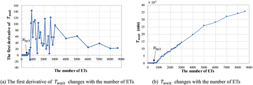
$T_{wait}$ is related to the number of CPs and the layout of CSs, and these factors are taken into consider in the simulation framework. According to the simulation results, $T_{wait}$ stays at about 0 until $N_{ET}$ grows to the threshold $N_{bp3}$, and then $T_{wait}$ begins to increase as shown in Figure 7(b), and $P_{bp3}$ is determined by the first derivative of $T_{wait}$ as shown in Figure 7(a). The piecewise regression function between $T_{wait}$ and $N_{ET}$ is shown as Equation (33) where $N_{bp3},\mu ,\sigma ,a_0,b_0,c_0$ are undetermined parameters.

Figure 7. The changing regulation of $T_{wait}$ under different fleet sizes.

Charging issues cost amount of time, so the operation efficiency is reduced, which is adverse to $r_{ET}$. On the other hand, ETs have a lower travel-mile-cost, and it is an obvious advantage to increase $r_{ET}$, which is formulated as Equations (35)(35) $r_{ET}=Incom{e}_{ET}-Cos{t}_{ET}$(35) –(37(37) $Cos{t}_{ET}=\frac{M_{ET}}{100}\ast e_{100}\ast Pric{e}_e$(37) ). In Equation (36), $M_0$ is the base mile of ETs, $i_0$ is the relative base fare, and $i_1$ is the price per kilometer beyond $M_0$. In Equation (37), $e_{100}$ is the electricity consumption per 100 km of an ET, and $Pric{e}_e$ is the unit price of electricity. All of the parameters above are set as Table 3 shows.

Table 3. Constant parameters in Equations (35)–(37).

Parameter	value
$e_{100}$	19.5 kW·h/100km
$M_0$	3 km (Liu 2020)
$i_0$	10 CNY (Liu 2020)
$i_1$	2 CNY/km (Liu 2020)
$Pric{e}_e$	1.5 CNY/kW·h (Liu 2020)

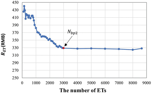
As shown in Figure 8, $R_{ET}$ declines with the number of ET growing to the system saturation point $N_{bp2}$. The piecewise regression function between $R_{ET}$ and $N_{ET}$ is shown as Equation (33) where $a_1,b_1,c_1,k_1,b_2$ are undetermined parameters. Taking $R_{ET}\ge R_{gasoline}$ as constraint condition refers to there is an intersection point $N_{is}$ of $R_{ET}$ and GTs’ revenue before $N_{bp2}$, thus the feasible section of $N_{ET}$ is {$N_{ET}|0\le N_{ET}\le N_{is},N_{ET}\in N\}$.

Figure 8. The changing regulation of $R_{ET}$ under different fleet sizes.

To solve multi-objective optimization problems, Multi-Objective Particle Swarm Optimization (MOPSO) (Coello and Lechuga 2002) is commonly adopted, which is used to solve the model. MOPSO adopts random mechanisms to update the particle location and realize the global search. This study implements this algorithm by taking $N_{ET}$ as the location of a particle to fit in the proposed MOOP model. The difference from MOPSO is that this study used the following strategy to avoid premature in the computation iteration of finding optimal substitution scale.

(38) $v_i\left(t\right)=\omega v_i\left(t-1\right)+c_{1}randf\left(x_{i_{pbest}}^t-x_i\right)+c_{2}randf\left(x_{gbest}^t-x_i\right)$(38)

(39) $x_i\left(t\right)=x_i\left(t-1\right)+v\left(t\right)$(39)

where, $t$ is the number of iterations, $v_i\left(t\right)$ is the speed of the particle i after the update of the t iteration, $v_i\left(t-1\right)$ is the speed of the particle $i$ of $t-1\hspace{0.17em}$ generation, and ω is the inertia weight. $c_1$ and $c_2$ refer to the individual learning factor and the group cognition factor, respectively. $x_i$ is the current position of the particle i and is described in this paper as the substitution scale of taxi electrification. $x_i\left(t-1\right)$ is the position of the particle $i$ of $t-1$ generation. $x_{i_{pbest}}^t$ is the historical optimal solution found for the particle$i$ up to generation$t$. $x_{gbest}^t$ is the historical optimal solution found by particle swarm search up to generation t. Here, the randf is a random function.

3. Case study of Zhengzhou City

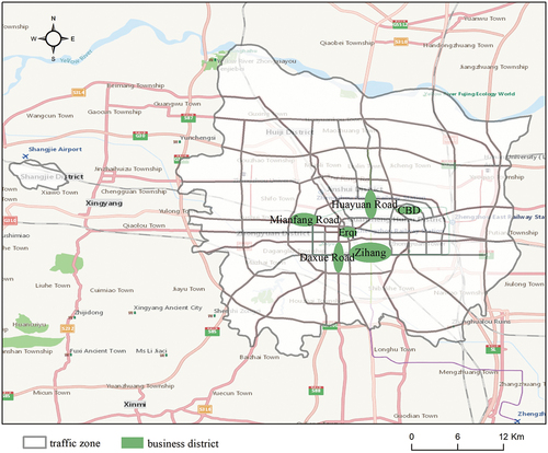
3.1. Study area and data

The study area (Figure 9) is Zhengzhou City, China. The data used in the simulation include city-wide road network datasets, daily GPS trajectory data of all 8650 taxicabs, and POI data of CS. Road network dataset comprises four kinds of the road segments (expressway, trunk road, sub-trunk road, and branch road). The trajectory data (July 1– 15 September 2018) record the location of taxis and other attributes versus time by a series of points. The attributes include $VID$, $V_s^{ET}$, $direction$, and $S_{occ}^{ET}$. 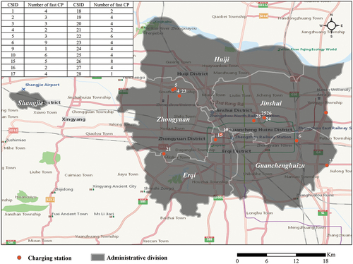The direction is indicated by azimuth, which is an integer between 0 and 360. The CS POI data involve the spatial distribution of CS and the number of CPs each CS contains, as shown in Figure 10.

Figure 9. Study area and the road network.

Figure 10. Distribution of CSs.

The datasets mentioned above were preprocessed at first. A network dataset in ArcGIS based on road network data was built. The network dataset is used to calculate the path distance between the entities in the simulation. The trajectory data are categorized into files according to the license plate number. Each file corresponds to the trajectory information of one taxi. These 8650 files help extract information regarding the operation of each taxi and the orders they complete to form the taxi and OD pools. The operation information includes the starting and ending time of taxis’ operations, which will be used to control the entry or exit of the ET entity from the simulation program, as well as the starting position of the taxi, which determines the position of the ET entity to be initialized in the simulation system. Compared with the random distribution, this real spatial distribution of ETs is more conducive to improve the simulation accuracy. The extracted order information includes the origin and destination, time and mileage costs, and income of the order. At last, the unique IDs to CSs and CPs were assigned for identification, and the inclusion relationship between them was established.

3.2. Obtaining the optimal substitute scale

3.2.1. System initialization and parameter settings

The initialization sets up an original state for the simulation, which involves the simulation environment and entities. First, the network analysis tool is activated to initialize the road network, which is used to plan the moving route of ETs. Then, charging facility entities are established according to their spatial position and quantity. And ET entities are set up by selecting fixed amount taxis from the initial state pool of taxis randomly. And this state pool is built up by the real operation data of GTs, which contains the initial position and operation state of these taxis. As for ETs’ initial battery state, we suppose ETs are fully recharged. Simultaneously, passenger entities are initialized in the corresponding position.

Table 4 gives the setting of parameters involved in the simulation program. The starting time of the system clock is 00:00, the ending time is 23:59, and the time step is 1 min in this simulation. The starting and ending times are set with limit of a day. The driving range of the ET is set to 240 km by referring to the performance parameters of BYD-E6 in the literature (MAIGOO 2018). The charging power of the CPs is set at 30 kW, which is the most common CP configuration (Autohome 2018).

Table 4. Setting of parameters involved in the simulation program.

Parameters	Symbol	Values
Simulation start time	$T_s$	0:00
Simulation end time	$T_e$	23:59
Simulation time step	$t$	1 min
Driving range of ETs	M	240 km
ET power consumption of 100 km	$e_{100}$	19.5 kW·h
Charging power of CPs	P	30 kW
Waiting time threshold of Passengers	${\epsilon }_{wait}$	12 min
Adjustment coefficient of target $SOC$ for charging	k	0.75

3.2.2. The optimize the substitution scale in simulations

In order to explore the range of the optimal substitution scale, by using the concept of linear fitting, this study conducted some simulation under the constraint of $N_{ET}$ growing from 0 to 8000 at the interval of 1000. The result shows the market is already saturated when $N_{ET}$ reaches 3000. To explore the changing rules of system status among range [0, 3000], further experiments were conducted at the interval of 100 within this range. Therefore, 30 kinds of substitution scales are simulated. Based on the simulation results, the parameters without dimension of the proposed MOOP model (see Table 5) are figured out according to the linear fitting approach.

Table 5. Parameters of the MOOP model derived from simulations.

Parameter	value	Parameter	value
$N_{bp1}$	800	$a_0$	−2.9e-03
$N_{bp2}$	3000	$b_0$	72.608
$N_{bp3}$	500	$c_0$	− 47,902
$\alpha$	−0.102	$a_1$	8e-06
$\beta$	1.6324	$b_1$	− 0.0622
$k$	−1e-06	$c_1$	439.71
$b$	0.8187	$k_1$	−3e-04
$\mu$	8e-16	$b_2$	328.84
$\sigma$	6.2366

In this study, the average revenue of GT $R_{gasoline}$ is about 395 CNY. According to the constraint $R_{ET}\ge R_{gasoline}$, the value range of $N_{ET}$ is solved as [0,811] through Equation (32). Supposing the OSS as $N^{\ast }$. When solving $N^{\ast }$ with the MOPSO algorithm, the number of iterations is set to 150, and the number of effective solutions reserved for each iteration is set to 200, of which the average value $N_i$ is considered as the temporary optimal value for iteration i. Further, as the number of iterations increases, $N_i$ tends to stabilize (Figure 11). According to the results, this study finds the final solution of this model as that $N^{\ast }$ = 778.

Figure 11. Iteration of optimal substitution scale of taxi electrification.

3.3. Simulation results of ETs, passengers and facilities under various electrification scale

3.3.1. Operating indices of ETs

This study used six indices to describe the operation of taxis, including OD number, income, total mileage, loaded mileage, occupied time, and the mileage utilization ratio of a taxi. These indices are calculated for GTs and ETs individually. The results in Figure 12 show that the indicators of GTs only fluctuate slightly with the increase in fleet size, and the operation performance is relatively stable. For GTs, they could complete approximately 27 orders every day on average and have the income about 488 CNY. Their total mileages per taxi are about 252 km per day. Within the total mileage, the loaded mileage is 183 km, and the serving time is about 383 min. The mileage utilization rate is about 0.7. As for the ETs, all indices decrease with the increasing number of ETs. Among these indices, the OD number, income, total mileage, and loaded mileage are below those of GTs because the running range is limited and the charging consumes a long time. Moreover, the loaded time of ETs is the same as GTs and even larger under the scenario of a small fleet size because ETs tend to select short-distance ODs for reducing the risk of stalling. These ODs are distributed mostly in urban areas with high crowd mobility and dense traffic. Therefore, it leads to a lower speed and longer loaded time of ETs. Furthermore, the mileage utilization of ETs is generally higher than GTs, which is due to the order allocation algorithm for ETs following the proximity principle, a common strategy adopted by ETs in reality to avoid power wastage caused by extremely long moving distances. In contrast, fuel consumption lightly contributes to the decision taken by GTs, which enables them to obtain objective income even though the mileage utilization is low. The comparison of mileage usage rate demonstrates that ETs are optional for ODs. Finally, the results of all indices present a downward trend with the increasing number of ETs, and the rate of decline gradually decreases. As the number of ETs increases to about 3000, these indices tend to be stable and ETs in the market are in a saturated state.

Figure 12. Comparison of operation indices under different ET fleet sizes.

3.3.2. Unmet travel demands of passengers

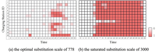
Unmet travel demands indicate ODs that are served by GTs under practical scenarios, however, are not met by ETs in the simulation. Here, we analyze this index under two situations, the saturation state of ETs in the market and the complete substitution state of GTs by ETs, to satisfy the requirements of decision makers. The ET fleet size corresponding to the saturation state is about 3000. The study area is divided into 100 traffic zones by main roads, as shown in Figure 13, for further revealing the spatial and temporal distribution of unmet travel demands. The number of unmet demands in each zone is then counted at an interval of one hour, and the statistical results are visualized, as shown in Figure 16 where the horizontal axis represents different substitution scales (778 and 3000). The vertical axis represents the time axis, and each sub-graph represents the amount of unmet travel demands in each zone at a certain time (hour granularity) under the relevant replacement scale. Under the saturation scene, the travel demands could not be satisfied on a large scale since 17:00, while the phenomenon appeared one hour earlier in the full electrification scene. This reflects the serving level declines because ETs spend more time on charging issues with the fleet size growing. This phenomenon spreads, intensifies and then reaches its peak at 21:00, which shows the same trend as temporal distribution of travel demands shown in Figure 14. In terms of spatial distribution, the spatial of travel demands’ distribution is shown in Figure 15. And regions containing a large amount of demands are earlier to appear unmet ones in Figure 16. Unmet travel demands in No. 108 zone located in the east of the city are the first to increase. It is far from the central area, however, contains the station with the largest passenger flow throughput in Zhengzhou. Subsequently, unmet travel demands among zones include the No. 31, 35, 75, 81, and 106 increase rapidly. These zones are adjacent to each other and include the largest commercial center, the Erqi business district, as shown in Figure 17. It then further extends to peripheral areas, including zones of No. 39 and 90 to the north of the center area, No. 110 to the northwest, and zone No. 13, 20, and 115 to the south. These zones include shopping malls, stations, universities, popular scenic spots, and other places with high crowd activity. The start time and regions of unmet travel demands provide more elaborate support for government regulation plans.

Figure 13. Division of traffic zones.

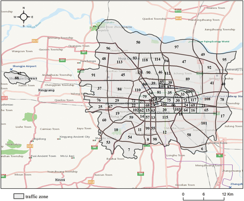
Figure 14. Temporal distribution of travel demands.

Figure 15. Spatial distribution of travel demands.

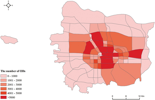
Figure 16. Spatial and temporal distribution of unmet travel demands.

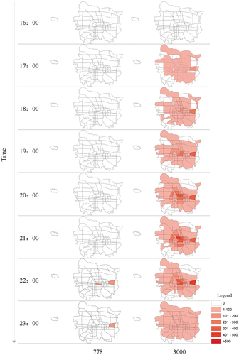
Figure 17. Distribution of business districts.

3.3.3. Usage state of charging facilities

The Usage rate $R_{occ}^{cs}$describes the busyness of a CS on the timescale of one hour. And $R_{occ}^{cs}$ is calculated by Equations (37)(37) $Cos{t}_{ET}=\frac{M_{ET}}{100}\ast e_{100}\ast Pric{e}_e$(37) and (38(38) $v_i\left(t\right)=\omega v_i\left(t-1\right)+c_{1}randf\left(x_{i_{pbest}}^t-x_i\right)+c_{2}randf\left(x_{gbest}^t-x_i\right)$(38) ). Relevant usage rates of CSs in one day under optimal substitution scenario (ET fleet size is 778) and saturation scenario (ET fleet size is 3000) are visualized as Figure 18(a,b) shows, respectively. And the shade of the color indicates the utilization rate.

Figure 18. The usage of CSs under optimal substitution scenario and saturation substitution scenario.

(40) $R_{occ}^{cp}=\frac{T_{occ}^{cp}}{60},R_{occ}^{cp}\in \left[0,1\right]$(40)

(41) $R_{occ}^{cs}=\frac{1}{n}\sum _{i=1}^n{R}_{occ}^{cp},R_{occ}^{cs}\in \left[0,1\right]$(41)

where $T_{occ}^{cp}$ represents occupied time of CP within one hour, $R_{occ}^{cp}$ is the time utilization of a CP, and n is the number of CPs contained in a CS.

It is obvious that CSs are much busier in scenario (b). And almost all the CSs reach high $R_{occ}^{cs}$ at 6:00 and continue until 22:00 because charging demands generated by 3000 ETs grow fast beyond the serving ability of CSs. As for scenario (a), the charging peak period is about 15:00 to 18:00. Many CSs only show slight busyness all day, and some CSs are busy only within charging peak period, reflecting that they are totally able to handle these charging demands. Moreover, it is noticed that No. 28 CS is always the first to get fully occupied and lasts for the longest time in two scenarios, which is because this CS is only equipped with one CP and needs to be expanded.

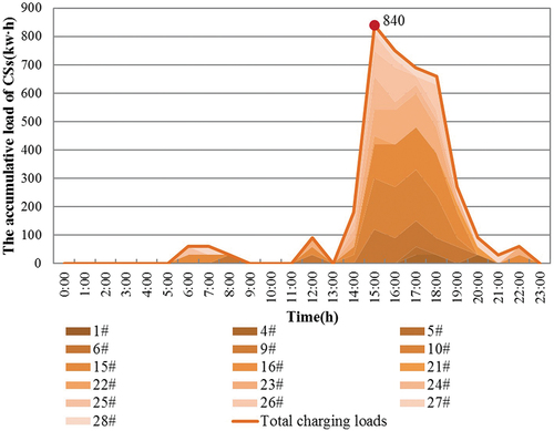
To quantify the charging pressure on the power grid brought by the ET fleet under the optimal substitution scenario, the stacked area chart of power consumption is shown in Figure 19, where the outermost contour exhibits the varying trend of total power consumption. The first peak appears at 6:00 ~ 7:00, this is the end of the first battery cycle of some ETs. These ETs prefer operating at night. And the battery cycle is defined as the period from an ET start operating with full-battery until it needs to recharge. After 13:00, the power consumption rapidly increases, peaking at 840 kW·h at 15:00. These charging demands are generated by the main body of ETs. They start operating in the early morning and need to recharge at noon. Then, the charging heat decreases gradually, reflecting that the charging facilities can absorb these charging demands.

Figure 19. Css loads in temporal and spatial scales.

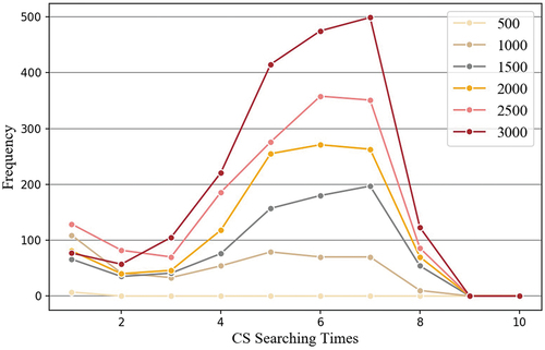
3.3.4. Charging queuing behavior of ETs

The searching times before the ET find a suitable one reflecting the sufficient degree of charging facilities relative to charging demands. Here, the frequencies of different searching times under various ET fleet sizes are compared in Figure 20. We can see that when the number of ETs is 500, all the ETs could directly access a free CP when they need to charge. As the number of ETs grows, the searching times for a suitable CS increase significantly. Moreover, the increment of the frequency corresponding to different searching times varies considerably. To find out the reason behind this, this study adopted the natural discontinuity point method to divide the searching times into three levels according to their increment of frequency as follows: low-value (0–3), median-value (4–7), and high-value (>7). These three levels refer to the charging difficulty from low to high. The frequency in the low-value area is mainly limited by the number of charging facilities. Thus, it does not vary considerably, irrespective of the number of ETs. The frequency in the high-value area is limited by the residual running range of ETs, which is rarely sufficient to search for CSs more than seven times. Therefore, this study concludes that the standard to measure the adequacy of charging facilities should depend on if a suitable CS could be found within three searching times.

Figure 20. Frequency for each CS searching times in various electrification scale.

4. Comparisons

4.1. Optimized results under different CS layouts

The proposed method firstly simulates the behaviors of the ET fleet, and further figures out the OSSs by the MOOP model. The case study applies this method under a fixed CS layout. This method is available for different CS layouts, which is practical for decision makers to understand the rationality of CS planning schemes. For example, according to the “Zhengzhou 13th five-year plan for electric vehicle charging infrastructure development” (ZZPG 2015), hereafter referred to as plan, we get information of CSs from 2016 to 2020, including the completion time, the number of CSs and CPs, and the locations of CSs. The quantities and relevant layouts of charging facilities from 2016 to 2020 are shown in Table 6 and Figure 21 respectively.

Figure 21. CS layouts from 2016 to 2020.

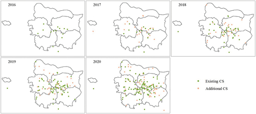
Table 6. The comparison of the quantity of charging facilities.

Time	The number of CSs	The number of CPs
2016	14	28
2017	36	72
2018	66	132
2019	106	212
2020	165	330

The growth of charging facilities could enlarge the market capacity of ETs. To further explore the OSSs under CS layouts from 2016 to 2020, we formulate and solve the relevant MOP models based on the method proposed in Section 2.2. And the iterations of OSSs from 2016 to 2020 based on the MOPSO algorithm are shown in Figure 22. The comparison of OSSs is drawn in Figure 23. Firstly, we can see there is a significant increase in OSS because of the growth of charging facilities. Then, the relationship between OSS and charging facilities is unlinear, which is because not only the quantity but also the spatial distribution of CSs also impacts the charging efficiency of the system. Moreover, charging facilities in plan until 2020 seem still not sufficient to realize the complete electrification. To sum up, this application on OSS under different CS layouts shows that the method proposed in this paper could supply a long-term support for government decision-making.

Figure 22. Iterations of OSS for 2016 to 2020 based on MOPSO algorithm.

Figure 23. The OSSs from 2016 to 2020.

4.2. Comparison with a mathematical optimization model

This study chose a mathematical model as the reference model (Sathaye 2014), which is developed to describe the relationship between system states and ET fleet size. As the influencing factors in this model are similar to those considered in the proposed model of this paper, the two models are highly comparable. The reference model takes the cost as the optimization objective as Equation (39), including the management cost of taxi companies, the time cost of passengers, the construction cost of charging facilities, and the distance cost of taxis.

The reference model supposes that the ETs should be in one of the three states (empty-driving, passenger-carrying, and charging), and the number of vehicles in each state is stable when the system is in equilibrium. Therefore, the number of ETs in each state could be firstly solved and then add them up to get the total number. Therefore, the reference model is mathematically expressed as Equations (39)(39) $x_i\left(t\right)=x_i\left(t-1\right)+v\left(t\right)$(39) -(49(49) $d=N\left[d_Q+d_I\right]+2d_C$(49) ) (Sathaye 2014).

$\mathrm{M}\mathrm{i}\mathrm{n}z=\left\{{\omega }_{Q}M\frac{d}{T}+{\omega }_{M}M+{\omega }_{Y}Y+{\omega }_{c}C\right\}+\frac{d_Q}{v}$

(42)

(43) $M=M_Q+M_E+M_C$(43)

(44) ${\omega }_Q=\frac{Q_f+Q_m}{\mathrm{\Lambda }\ast P}$(44)

(45) ${\omega }_M=\frac{Q_{M0}+Q_{M1}}{\mathrm{\Lambda }\ast P}$(45)

(46) ${\omega }_Y=\frac{Q_{Y0j}+Q_{Y1j}}{\mathrm{\Lambda }\ast P}$(46)

(47) ${\omega }_C=\frac{Q_{C0j}+Q_{C1j}}{\mathrm{\Lambda }\ast P}$(47)

(48) $P=\frac{GD{P}_p}{Q_{AWH}}$(48)

(49) $d=N\left[d_Q+d_I\right]+2d_C$(49)

(50) $T=N\left[b_1+b_2+\frac{d_Q}{v}\right]+N\left[\frac{d_c}{Nv}+\frac{d_I}{v_I}\right]+\left[b_3+\frac{d_c}{v}\right]$(50)

(51) $d_C=0.38kD/\sqrt{Y}$(51)

(52) $\mathrm{\Lambda }=\frac{M_E}{\left[\frac{d_C}{Nv}+\frac{d_I}{v_I}\right]}=\frac{M_Q}{\left[b_1+b_2+\frac{d_Q}{v}\right]}=\frac{N{M}_C}{\left[b_3+\frac{d_C}{v}\right]}$(52)

where the parameters involved in the model are explained in Table 7, and the values are set considering the specific situation of the research area.

Table 7. Parameters mentioned in the model.

Variables	Unit	Definition	Value
${\omega }_Q$	pax h/km	Distance cost factor	Equation (44)(44) ${\omega }_Q=\frac{Q_f+Q_m}{\mathrm{\Lambda }\ast P}$(44)
${\omega }_M$	pax h/h	Operating time cost factor	Equation (45)(45) ${\omega }_M=\frac{Q_{M0}+Q_{M1}}{\mathrm{\Lambda }\ast P}$(45)
${\omega }_Y$	pax h/site	Fixed CS cost factor	Equation (46)(46) ${\omega }_Y=\frac{Q_{Y0j}+Q_{Y1j}}{\mathrm{\Lambda }\ast P}$(46)
${\omega }_C$	pax h/port	Variable CS cost facto	Equation (47)(47) ${\omega }_C=\frac{Q_{C0j}+Q_{C1j}}{\mathrm{\Lambda }\ast P}$(47)
$Q_f$	CNY/[veh×km]	Fuel cost	0.14 (BK 2012)
$Q_m$	CNY/[veh×km]	Fleet maintenance cost	0.06 (Autohome 2018)
$Q_{M0}$	CNY/[veh×h]	Fleet depreciation cost	2.8 (HQEW 2016)
$Q_{M1}$	CNY/[veh×h]	Agency operating cost per time	12.36 (HQEW 2016)
$Q_{Y0j}$	CNY/[site×h]	Station installation fixed site cost	4.864
$Q_{Y1j}$	CNY/[site×h]	Station maintenance fixed site cost	2.432
$Q_{C0j}$	CNY/[site×h]	Station installation variable port cost	0.96
$Q_{C1j}$	CNY/[site×h]	Station maintenance variable port cost	0.486
$\mathrm{\Lambda }$	trips/h	Spatially homogenous peak-period pickup and drop-off demand	2
$GD{P}_p$	CNY/ppl×y	GDP per capita	78,003.73(GAOKAOHELP 2018)
$Q_{AWH}$	h	Average working hour annually	2300 (CNBS 2018)
$P$	CNY/pax h	Passenger value of time	Equation (48)(48) $P=\frac{GD{P}_p}{Q_{AWH}}$(48)
$M$	taxis	Number of taxis in the fleet	Equation (43)(43) $M=M_Q+M_E+M_C$(43)
$M_Q$	taxis	Number of taxis servicing trips	Equation (43)(43) $M=M_Q+M_E+M_C$(43)
$M_E$	taxis	Number of empty taxis	Equation (43)(43) $M=M_Q+M_E+M_C$(43)
$M_C$	taxis	Number of charging taxis	Equation (43)(43) $M=M_Q+M_E+M_C$(43)
$d$	km	Vehicle range for BEVs	240
$d_Q$	km	Expected distance traveled by a taxi while servicing a trip	7
$d_C$	km	Expected distance traveled by taxis while driving to a CS	Equation (49)(49) $d=N\left[d_Q+d_I\right]+2d_C$(49)
$d_I$	km	Expected distance traveled by a taxi while idle	Equation (49)(49) $d=N\left[d_Q+d_I\right]+2d_C$(49)
$T$	h	Expected cycle time	Equation (50)(50) $T=N\left[b_1+b_2+\frac{d_Q}{v}\right]+N\left[\frac{d_c}{Nv}+\frac{d_I}{v_I}\right]+\left[b_3+\frac{d_c}{v}\right]$(50)
$Y$	sites	Number of CS sites	85
$C$	ports	Number of CS ports	28
$k$		Routing factor	1.270
$D$	km	Length of the side of the square service region	32(HNPG 2018)
$N$	trips	Number of trips serviced between charging	$Nϵ\left[0,\frac{d}{d_Q}\right)$,
$v$	Km/h	Average speed traveled by taxis	28.5
$v_I$	Km/h	Speed traveled by an idle taxi	10
$b_1$	h	Boarding time	0.0042
$b_2$	h	Alighting time	0.017
$b_3$	h	Time spent at a CS by a taxi	1

This study adopts the exhaustive method to list all of the $M_E$ and the corresponding cost under the optimal taxi fleet to elect the optimal $M_E$ with the minimum cost. Table 8 shows the distribution of the number of ETs in the three kinds of state solved by the reference model.

Table 8. Optimal number of the reference model.

Empty-driving ETs	Passenger-carrying ETs	Charging ETs	Total number
9	209	57	295

To make a further comparison, this study takes three indices, including the empty-driving ratio, the gasoline saved, and the utilization rate of CPs, to represent the system state under the two substitution solutions as Table 9 shows. The actual empty-driving ratio of taxi fleet is about 60% according to the taxi trajectory data, and this index of the proposed approach is about 54%, while the index of the reference model is about 10%. Therefore, the proposed approach shows a more moderate and reasonable description of the ETs’ system. On the other hand, the saved gasoline of the two models is 11,018.7 L/d and 4380.8 L/d, respectively, demonstrating that the proposed approach would bring much more benefits to energy and the environment. In the aspect of the utilization of CPs, the two models are similar. In short, compared with the reference model, the proposed approach shows a more reasonable abstraction of the ET’s system, and its solution brings more benefits to resources and the environment. Moreover, the proposed approach is suitable for dynamic application scenarios and could show more details of the system both in spatial and timescales, while mathematical modeling methods under a static assumption are weak in considering spatiotemporal factors.

Table 9. Comparison of the two solutions.

Empty-driving ratio (%)		Gasoline saved (L/d)		Utilization rate of CPs
Proposed approach	Reference model	Proposed approach	Reference model	Proposed approach	Reference model
54	10	11,018.7	4380.8	0.66	0.67

5. Conclusion and discussion

This paper presents an approach based on the discrete-event to simulate the behaviors of ETs in the market, and eventually to estimate the substitution of GTs by ETs under various scales. This approach considers real datasets, including road network, GPS trajectory data, and CS POI data, to construct a realistic virtual scene for the simulation, which is easily expanded and updated. The contribution of the paper could be summarized as follows: (1) a discrete-event-based approach is proposed to simulate the spatiotemporal behavior of ETs, which supports to obtain the quantitative impacts on multiple participants caused by the number of ETs. (2) the status changing law of entities under different substitution scales in the study area, such as the operating indices of ETs, the unsatisfied travel requirements of passengers, and the usage state of charging facilities are revealed, which provide practical guidance to the decision-making of the optimal substitution scale, and (3) a multi-objective optimization model is proposed to optimize quantity of ETs in cities, which help to find the optimal substitution scale of GTs by ET. This proposed approach provides scientific support for policy-making, exhibiting crucial practical significance in the current context of taxi electrification. Moreover, the proposed approach could be used in many other application scenarios, such as identifying a better CS planning scheme by replacing the input datasets of the road network or charging facilities. Based on the spatiotemporal distribution of charging demands obtained by simulation, studies on CS location and capacity determination could be conducted. Further, the system state under the coexistence of multiple vehicles can also be simulated by considering the behavior of other types of vehicles.

The simulation framework proposed in this paper can provide a general tool for different cities to solve the problem of taxi electrification-scale optimization and provide support for decision makers. In order to achieve this goal, on the one hand, the simulation framework has great flexibility in design and provides many adjustable parameters. The entities’ attributes, the triggering conditions of behaviors and events can be set according to the specific situation of the city. On the other hand, input data of the simulation framework are easy to obtain, mainly including network analysis data set generated based on urban vector road network data, gasoline taxi track data, longitude and latitude of charging stations and the number of charging piles.

While this study provides a practical tool to support the policy-making for the urban taxi electrification problem, there are still several further improvements. First, from the perspective of travel demands, only ODs that have been satisfied in real life are considered in the simulation. Those unmet ODs get neglected because of the difficulty in collecting the necessary data. Second, as for simulation rules, it is necessary to supplement the non-operational behavior of taxis, such as dining and shift taking. Further, attention should be paid to the impact of such behaviors on drivers’ operation and recharging decisions, which involve the experience of the drivers. Third, the simulation does not consider subsidy policies for ETs, which plays a vital role for promoting the popularization of ETs at the present stage. Fourth, owing to the lag in the charging facilities, taxi electrification should still be further improved. In other words, ETs and GTs will still coexist for a long time. Therefore, an effective business model for ETs to lessen their disadvantages in market competition should be designed, and the effectiveness of the model through simulations should be verified.

Disclosure statement

No potential conflict of interest was reported by the author(s).

Additional information

Funding

The research was supported in part by the National Natural Science Foundation of China [Grant 41771473] and Fundamental Research Funds for the Central Universities [Grant 2042020kfxg24].

Notes on contributors

Zhixiang Fang

Zhixiang Fang is currently a Professor with the State Key Laboratory of Information Engineering in Surveying, Mapping and Remote Sensing, Wuhan University. His research interests include crowd dynamics-oriented observation, human mobility, and intelligent navigation.

Xiaofan Wang

Xiaofan Wang received MS degree from Wuhan University. Her research interests include geospatial big data analytic and smart transportation.

Ying Zhuang

Ying Zhuang received MS degree from Wuhan University. She was also a Visiting Scholar with the Singapore-MIT Alliance for Research and Technology (SMART). Her research interests include geospatial big data analytic and smart transportation.

Xianglong Liu

Xianglong Liu is currently a researcher with Key Laboratory of Advanced Public Transportation Science, China Academy of Transportation Sciences. His research interests include smart public transportation, and MaaS.

References

- Autohome. 2018. “How About the Maintenance Cost of Byde6?” Accessed 10 November 2021. https://club.autohome.com.cn/bbs/thread/fc1c66cf57c3ee6d/77326938-1.html
- Autotimes. 2016. “How Does BYDE6 Charge and How Many Kilometers Is the Maximum Range?” Accessed 15 December 2021. https://www.autotimes.com.cn/market/201612/news_720751.html
- Azadfar, E., V. Sreeram, and D. Harries 2015. “The Investigation of the Major Factors Influencing Plug-In Electric Vehicle Driving Patterns and Charging Behavior.” Renewable and Sustainable Energy Reviews 42 (C): 1065–1076. doi:10.1016/j.rser.2014.10.058.
- Bischoff, J., and M. Maciejewski 2014. “Agent-Based Simulation of Electric Taxicab Fleets.” Transportation Research Procedia 4: 191–198. doi:10.1016/j.trpro.2014.11.015.
- Bi, J., W. Zhang, X. Zhao, and T. Zhang 2017. “Charging Behavior Analysis of Electric Logistic Vehicle Based on Data Driven.” Journal of Transportation Systems Engineering 17 (1): 106–111. doi:10.16097/j.cnki.1009-6744.2017.01.016.
- BK. 2012. “How Much Does Byde6 Cost per Kilometer?” Accessed 15 November 2021. https://zhidao.baidu.com/question/385794817.html
- Brodeur, A., and K. Nield 2018. “An Empirical Analysis of Taxi, Lyft and Uber Rides: Evidence from Weather Shocks in NYC.” Journal of Economic Behavior & Organization 152 (C): 1–16. doi:10.1016/j.jebo.2018.06.004.
- CNBS. 2018. “China’s National Bureau of Statistics, China Works 9.2 Hours per Person, Almost the First in the World.” Accessed 27 September 2021. https://www.sohu.com/a/249636420_100176388
- Coello, C., and M. S. Lechuga 2002. “MOPSO: A Proposal for Multiple Objective Particle Swarm Optimization.” Paper presented at the IEEE Congress on Evolutionary Computation, Honolulu, May 12–17. doi:10.1109/CEC.2002.1004388.
- Dallinger, D., and M. Wietschel 2012. “Grid Integration of Intermittent Renewable Energy Sources Using Price-Responsive Plug-In Electric Vehicles. Renew.” Renewable & Sustainable Energy Reviews 16 (5): 3370–3382. doi:10.1016/j.rser.2012.02.019.
- GAOKAOHELP. 2018. “Henan’s per Capita GDP Ranking in 2018.” Accessed 27 September 2021. http://www.creditsailing.com/JingJiZhengCe/647365.html
- Gasparini, M. 1997. “Markov Chain Monte Carlo in Practice.” Technometrics 39 (3): 338. doi:10.1080/00401706.1997.10485132.
- Gong, H., Y. Zou, Q. Yang, J. Fan, F. Sun, and D. Goehlich 2018. “Generation of a Driving Cycle for Battery Electric Vehicles: A Case Study of Beijing.” Energy 150 (C): 901–912. doi:10.1016/j.energy.2018.02.092.
- Grüger, F., L. Dylewski, M. Robinius, and D. Stolten 2018. “Carsharing with Fuel Cell Vehicles: Sizing Hydrogen Refueling Stations Based on Refueling Behavior.” Applied Energy 228 (C): 1540–1549. doi:10.1016/j.apenergy.2018.07.014.
- Hastings, W. K. 1970. “Monte Carlo Sampling Methods Using Markov Chains and Their Applications.” Biometrika 57 (1): 97–109. doi:10.1093/biomet/57.1.97.
- He, X., Y. Wu, S. Zhang, M.A. Tamor, T.J. Wallington, and W. Shen 2016. “Individual Trip Chain Distributions for Passenger Cars: Implications for Market Acceptance of Battery Electric Vehicles and Energy Consumption by Plug-In Hybrid Electric Vehicles.” Applied Energy 180 (15): 650–660. doi:10.1016/j.apenergy.2016.08.021.
- HNPG. 2018. “Henan People’s Government, Administrative Divisions of Zhengzhou.” http://www.henan.gov.cn/2006/09-08/231049.html. Accessed 30 September 2021.
- HQEW. 2016. Electric Taxi Charge Three Times a Day, Charging Inconvenience Constraints Development. Accessed 30 August 2021. https://tech.hqew.com/news_782418
- Kaltschmitt, M., W. Streicher, and A. Wiese 2007. Renewable Energy. Berlin: Springer. doi:10.1007/3-540-70949-5_6.
- Keler, A., J. M. Krisp, and L. Ding 2019. “Extracting Commuter-Specific Destination Hotspots from Trip Destination Data – Comparing the Boro Taxi Service with Citi Bike in NYC.” Geo-Spatial Information Science 23 (2): 141–152. doi:10.1080/10095020.2019.1621008.
- Kong, D., D. Ma, and M. Wang 2016. “A Simulation Study of Upgrading Urban Gasoline Taxis to Electric Taxis.” Energy Procedia 104: 390–395. doi:10.1016/j.egypro.2016.12.066.
- Liang, X., G. Correia, and B. van Arem 2016. “Optimizing the Service Area and Trip Selection of an Electric Automated Taxi System Used for the Last Mile of Train Trips.” Transportation Research Part E: Logistics and Transportation Review 93: 115–129. doi:10.1016/j.tre.2016.05.006.
- Li, B., Z. Cai, L. Jiang, S. Su, and X. Huang 2019. “Exploring Urban Taxi Ridership and Local Associated Factors Using GPS Data and Geographically Weighted Regression.” Cities 87: 68–86. doi:10.1016/j.cities.2018.12.033.
- Li, Z., L. Jiao, B. Zhang, G. Xu, and J. Liu 2021a. “Understanding the Pattern and Mechanism of Spatial Concentration of Urban Land Use, Population and Economic Activities: A Case Study in Wuhan, China.” Geo-Spatial Information Science 24 (4): 678–694. doi:10.1080/10095020.2021.1978276.
- Lioris, E., G. Cohen, and D. Arnaud 2009. “Simulation and Evaluation of Collective Taxi Systems.” IFAC Proceedings Volumes 42 (15): 263–270. doi:10.3182/20090902-3-us-2007.0014.
- Li, L., T. Pantelidis, J. Chow, and S. E. Jabari 2021b. “A Real-Time Dispatching Strategy for Shared Automated Electric Vehicles with Performance Guarantees.” Transportation Research Part E: Logistics and Transportation Review 152 (C): 102392. doi:10.1016/j.tre.2021.102392.
- Liu, X.Y.D. 2020. “2021 Zhengzhou Taxi Fare Standard Adjustment Policy.” Accessed 5 August 2021. https://zz.bendibao.com/traffic/20201225/76676.shtm
- Liu, X., and S. Liu 2016. “The Great Leap Forward Dilemma of the New Deal for Energy Taxi in Hengshui.” Decision-Making 10: 82–84. http://qikan.cqvip.com/Qikan/Article/Detail?id=670425755
- Liu, H., Y. Zou, Y. Chen, and J. Long 2021a. “Optimal Locations and Electricity Prices for Dynamic Wireless Charging Links of Electric Vehicles for Sustainable Transportation.” Transportation Research Part E: Logistics and Transportation Review 152: 102187. doi:10.1016/j.tre.2020.102187.
- Li, X., E. Wang, and C. Zhang 2014. “Prediction of Electric Vehicle Ownership Based on Gompertz Model.” In Published in: 2014 IEEE International Conference on Information and Automation (ICIA), Hailar, July 28–30. doi:10.1109/ICInfA.2014.6932631.
- Lu, J., and W. Wang 2004. “A Method to Determine Urban Taxi Ownership.” Journal of Traffic and Transportation Engineering 4 (1): 92–95. doi:10.3321/j.issn:1671-1637.2004.01.023.
- MAIGOO. 2018. “[Charging Pile Power] What Is the Power of Quick Charging Pile? State Grid Charging Pile Power Description.” Accessed 10 August 2021. www.maigoo.com/goomai/210268.html
- Meng, X., L. Liu, H. Hui, X. Feng, and G. Chen 2016. “Effects of Discharge Depth on Battery Life.” Auto Sci-Tech 3: 47–51. doi:10.3969/j.issn.1005-2550.2016.03.008.
- Noel, L., Z. D. R. Gerardo, B. K. Sovacool, and J. Kester 2019. “Fear and Loathing of Electric Vehicles: The Reactionary Rhetoric of Range Anxiety.” Energy Research & Social Science 48 (1): 96–107. doi:10.1016/j.erss.2018.10.001.
- Paulista, C. R., T. A. Peixoto, and D. Jose 2019. “Modeling and Discrete Event Simulation in Industrial Systems Considering Consumption and Electrical Energy Generation.” Journal of Cleaner Production 224 (2): 864–880. doi:10.1016/j.jclepro.2019.03.248.
- Rao, R., X. Zhang, X. Jian, and L. Ju 2015. “Optimizing Electric Vehicle Users’ Charging Behavior in Battery Swapping Mode.” Applied Energy 155 (1): 547–559. doi:10.1016/j.apenergy.2015.05.125.
- Sathaye, N. 2014. “The Optimal Design and Cost Implications of Electric Vehicle Taxi Systems.” Transportation Research Part B: Methodological 67 (C): 264–283. doi:10.1016/j.trb.2014.05.009.
- Shareef, H., M. M. Islam, and A. Mohamed 2016. “A Review of the Stage-Of-The-Art Charging Technologies, Placement Methodologies, and Impacts of Electric Vehicles.” Renewable and Sustainable Energy Reviews 64 (C): 403–420. doi:10.1016/j.rser.2016.06.033.
- Skippon, S., and J. Chappell 2019. “Fleets’ Motivations for Plug-In Vehicle Adoption and Usage: U.K. Case Studies.” Transportation Research Part D: Transport and Environment 71: 67–84. doi:10.1016/j.trd.2018.12.009.
- SMN. 2018. “The Southern Metropolis News, Shenzhen: 80% of Electric Taxi Drivers Surveyed Believe Charging Affects Their Daily Operations.” Accessed 17 August 2021. www.sohu.com/a/237245054_540811
- Sun, L., Y. Huang, S. Liu, Y. Chen, L. Yao, and A. Kashyap 2017. “A Completive Survey Study on the Feasibility and Adaptation of EVs in Beijing, China.” Applied Energy 187 (C): 128–139. doi:10.1016/j.apenergy.2016.11.027.
- Teodorovic, D. 2003. “Transport Modeling by Multi-Agent Systems: A Swarm Intelligence Approach.” Transportation Planning and Technology 26 (4): 289–312. doi:10.1080/0308106032000154593.
- Tian, Z., Y. Wang, C. Tian, F. Zhang, L. Tu, and C. Xu 2014. “Understanding Operational and Charging Patterns of Electric Vehicle Taxis Using GPS Records.” In Published in: 2014 IEEE 17th International Conference on Intelligent Transportation Systems (ITSC), Qingdao, August 8–11. doi:10.1109/ITSC.2014.6958086.
- Tu, W., P. Santi, T. Zhao, X. He, Q. Li, L. Dong, T. J. Wallington, and C. Rattic 2019. “Acceptability, Energy Consumption, and Costs of Electric Vehicle for Ride-Hailing Drivers in Beijing.” Applied Energy 250 (C): 147–160. doi:10.1016/j.apenergy.2019.04.157.
- Veneri, O. 2017. Technologies and Applications for Smart Charging of Electric and Plug-In Hybrid Vehicles. Berlin: Springer. doi:10.1007/978-3-319-43651-7.
- Wang, R., Y. Wu, W. Ke, S. Zhang, B. Zhou, and J. Hao 2015. “Can Propulsion and Fuel Diversity for the Bus Fleet Achieve the Win–win Strategy of Energy Conservation and Environmental Protection?” Applied Energy 147 (C): 92–103. doi:10.1016/j.apenergy.2015.01.107.
- Wang, Z., J. Zhang, P. Liu, C. Qu, and X. Li 2019. “Driving Cycle Construction for Electric Vehicles Based on Markov Chain and Monte Carlo Method: A Case Study in Beijing.” Energy Procedia 158 (1): 2494–2499. doi:10.1016/j.egypro.2019.01.389.
- Wong, K., S. Wong, and H. Yang 2001. “Modeling Urban Taxi Services in Congested Road Networks with Elastic Demand.” Transportation Research Part B: Methodological 35 (9): 819–842. doi:10.1016/S0191-2615(00)00021-7.
- Wu, H., Z. Gui, and Z. Yang 2020. “Geospatial Big Data for Urban Planning and Urban Management.” Geo-Spatial Information Science 23 (4): 273–274. doi:10.1080/10095020.2020.1854981.
- Xydas, E., C. Marmaras, and L. M. Cipcigan 2016. “A Multi-Agent Based Scheduling Algorithm for Adaptive Electric Vehicles Charging.” Applied Energy 177 (1): 354–365. doi:10.1016/j.apenergy.2016.05.034.
- Yang, J., J. Dong, Z. Lin, and L. Hu 2016. “Predicting Market Potential and Environmental Benefits of Deploying Electric Taxis in Nanjing, China.” Transportation Research Part D: Transport and Environment 49: 68–81. doi:10.1016/j.trd.2016.08.037.
- Yang, Y., C. Hua, and S. Zhang 2012. “A Prediction Model of the Number of Taxicabs Based on Wavelet Neural Network.” Procedia Environmental Sciences 12 (B): 010–1016. doi:10.1016/j.proenv.2012.01.380.
- Yang, H., and S. Wong 1998. “A Network Model of Urban Taxi Services.” Transportation Research Part B: Methodological 32 (4): 235–246. doi:10.1016/s0191-2615(97)00042-8.
- Yang, H., S. Wong, and K. Wong 2002. “Demand–supply Equilibrium of Taxi Services in a Network Under Competition and Regulation.” Transportation Research Part B: Methodological 36 (9): 799–819. doi:10.1016/S0191-2615(01)00031-5.
- Zhang, X., and Y. Liu 2015. “The City Taxi Quantity Prediction via GM-BP Model.” In Published in: The 5th Annual IEEE International Conference on Cyber Technology in Automation, Control and Intelligent Systems, Shenyang, June 8–10. doi:10.1109/CYBER.2015.7288183.
- Zhao, W., Y. Qin, Y. Dong, L. Zhang, and W. Zhu 2014. “Social Group Architecture Based Distributed Ride-Sharing Service in VANET.” International Journal of Distributed Sensor Networks 10 (3): 1–8. doi:10.1155/2014/650923.
- ZZPG. 2015. “Zhengzhou People’s Government, Zhengzhou 13th Five-Year Plan for Electric Vehicle Charging Infrastructure Development.” Accessed 14 August 2021. http://www.doc88.com/p-0079696056708.html