Compact and indexed representation for LiDAR point clouds

ABSTRACT

LiDAR devices are capable of acquiring clouds of 3D points reflecting any object around them, and adding additional attributes to each point such as color, position, time, etc. LiDAR datasets are usually large, and compressed data formats (e.g. LAZ) have been proposed over the years. These formats are capable of transparently decompressing portions of the data, but they are not focused on solving general queries over the data. In contrast to that traditional approach, a new recent research line focuses on designing data structures that combine compression and indexation, allowing directly querying the compressed data. Compression is used to fit the data structure in main memory all the time, thus getting rid of disk accesses, and indexation is used to query the compressed data as fast as querying the uncompressed data. In this paper, we present the first data structure capable of losslessly compressing point clouds that have attributes and jointly indexing all three dimensions of space and attribute values. Our method is able to run range queries and attribute queries up to 100 times faster than previous methods.

KEYWORDS:

• 3D point clouds
• lossless compression
• indexing

1. Introduction

By scanning the entire field of view with a laser beam at a high speed, a LiDAR sensor produces a dense cloud of points that can be used to determine the 3D geometry of the objects around the sensor. The cost of LiDAR sensors has dropped dramatically in recent years. Hence, they have been included in autonomous cars (Royo and Ballesta-Garcia 2019) to map the environment and identify obstacles or in consumer devices such as the 2020 iPad Pro to more accurately focus images and videos in low-light conditions and reduce capture time.¹ As a result, the applications that use LiDAR-acquired point clouds are increasing, and thus, large data sets are being produced that require large computational resources to be processed.

In this work, we focus on LiDAR data, but it can be generalized to any scenario where i) we need to store point clouds in the 3D space, ii) those points have attribute values, such as color, intensity, scan angle, etc., and iii) it is relevant to query those data combining the 3D space and the attribute values associated with the points. Traditionally, compression of point clouds is tied to image compression, but in this field, the aforementioned query capacity is not supported.

In the traditional setup, data reside on disk. Every time a given datum is desired, an I/O transfer between disk and main memory is required, which is extremely slow when compared to CPU speeds. Although important improvements in processors and parallel computing are appearing, disk accesses still represent a bottleneck. Moreover, the increase in the size of the datasets requires the development of new strategies to obtain also improvements in processing time or scalability. Hence, many approaches that compress the data have appeared not only to save disk space but also to reduce transmission time in networks.

Dewitt et al. (1984) proposed to get rid of disk accesses in database management systems and keep all data in main memory all the time. This gave rise to a new line of research called “in-memory data management” (Plattner 2009; Plattner and Zeier 2012). Although main memory is getting cheaper, thus, allowing more data to be represented and processed in main memory, the size of current datasets is growing at a faster pace. This has promoted the use of compression with the goal of fitting larger datasets in main memory. From a compression point of view, the compression methods for this scenario must have different characteristics with respect to classic archival methods. In particular, access to the data must be very fast so as not to impair processing times. That is, compression and decompression times are now more important than a high compression capability.

With this goal in mind, a new research field called compact data structures (Navarro 2016) has emerged. These are compression methods that go one step further. The traditional methods require decompressing large parts of the dataset when a given datum is needed (e.g. compressing a column of a table using traditional algorithms such as deflate requires decompressing the whole column when a value is required). In compact data structures, the desired data can be accessed without any previous decompression. This speeds up access times. Moreover, to match the access times of uncompressed data structures, compact data structures are usually equipped with indexes within the compressed data, and the index itself is also compressed.

In this paper, we present two compact data structures to store point clouds having additional attributes: ${\mathrm{k}}^3-\mathrm{l}\mathrm{i}\mathrm{d}\mathrm{a}\mathrm{r}$ and ${\mathrm{k}}_{\mathrm{i}}^3-\mathrm{l}\mathrm{i}\mathrm{d}\mathrm{a}\mathrm{r}$. They reside in main memory all the time and thus they do not access the disk. In addition, they index all dimensions, the space, and the attributes, so that they obtain remarkable query times. The trade-off is a lower performance in information compression.

The rest of the paper is structured as follows. Section 2 describes the LAS and LAZ file formats and the background knowledge required to understand our data structures. Section 3 describes the ${\mathrm{k}}^3-\mathrm{l}\mathrm{i}\mathrm{d}\mathrm{a}\mathrm{r}$ to represent point clouds including a 3D spatial index. Section 4 describes the ${\mathrm{k}}_{\mathrm{i}}^3-\mathrm{l}\mathrm{i}\mathrm{d}\mathrm{a}\mathrm{r}$ that includes and additional index over the attributes. Section 5 presents an evaluation of the data structures comparing their time and space requirements against the LAZ file format. Finally, Section 6 presents the conclusions and future work.

2. Related work

2.1. LiDAR

LiDAR (Light Detection and Ranging) technology has been used to classify and recognize objects in many different application fields during the last four decades (Dong and Chen 2017). LiDAR sensors work by shooting a laser beam that is reflected by nearby objects and the time it takes for the reflection of the beam to return is used to compute the location of a point in the 3D space. Furthermore, additional information can be attached to the point, such as the intensity of the reflection, the georeferenced position of the point if the sensor includes a GPS sensor or an inertial navigation system, or the color of the point if the sensor includes a visible-light sensor.

LiDAR point clouds are used, for example, to classify and recognize objects in the natural environment (e.g. forests (Hyyppa et al. 2018), landslides (Jaboyedoff et al. 2012)), in urban environments (Wang, Peethambaran, and Chen 2018), or even underwater (Palomer et al. 2018). The following sections describe the LAS and LAZ formats that are commonly used to store and process LiDAR point clouds.

2.1.1. LAS and LAZ formats

The American Society for Photogrammetry and Remote Sensing (2019) defined the LASer (LAS) file format to store clouds of LiDAR points. It is an open binary format composed of a header block that describes general information about the point cloud (e.g. number of points, bounding box, etc.), optional variable-length records to describe additional information such as georeferencing information or other metadata, and fixed-length point records. There are eleven types of these point records. Each type includes coordinates (i.e. $x$, $y$, and $z$), and several other attributes, such as the intensity, color, time, etc. The exact additional values depend on the record type.

Even though the coordinates are stored as scaled and offset integers, LAS files are usually large. Therefore, a lossless compressed version of the LAS file format, called LAZ or LASzip (Isenburg 2013), was defined.

Using common point compression terminology, LAZ is a lossless, non-progressive, streaming, and order-preserving compressor. Non-progressive means that it is not capable of providing a faster lower resolution image; streaming means that it is capable of compressing the data as they arrive, that is, it does not need to have all the points before starting the compression; order-preserving means that it keeps the original order of the points. Additionally, LAZ provides, to some extent, random access, that is, LAZ is capable of decompressing parts of the data without having to start the decompression from the beginning.

The LAZ file format independently compresses points in chunks of 50,000 points, by default. This can be configured, yielding different compression levels, but (Isenburg 2013) advises values between 5,000 and 50,000. A chunk table at the end of the compressed file gives the position of the initial byte of the chunk in the original uncompressed array.

LAZ neither compresses the header nor the variable-length records. These parts are small and barely compressible. For compressing the $x$, $y$, and $z$ coordinates, each chunk stores the first point uncompressed, and the rest are compressed with a context-based arithmetic compressor (Ida Mengyi 2006). Instead of compressing the absolute coordinates, for a given point, it compresses the difference between the actual value and a prediction based on the previous points. This is the key factor causing LAZ to not have real random access. To decompress a given point, LAZ needs to have the previous points uncompressed up to the first uncompressed point of the chunk. However, each chunk can be decompressed independently, and thus, unlike traditional compression methods, it allows, to some extent, random access decompression. To obtain a given point or set of points, we can only decompress the chunks where they are located. Moreover, range (cube) queries can be solved by storing the bounding box of each chunk, in the chunk table. Regarding the attributes, each one has its own compression method, but some of them also need to have the uncompressed versions of the previous points.

The LAZ file format obtains notable results in compression, achieving compression ratios similar to or better than general-purpose compressors such as ZIP or RAR. In addition, since LAZ does not alter the original order and it does not use an octree, it can start the compression as the points arrive. This type of compression yields a low memory footprint because once the points are compressed they can be output to disk, freeing up the main memory.

2.1.2. LAS index

One advantage of the LAZ file format is that the response times can be improved thanks to the possibility of adding an adaptive quadtree that indexes the points, which is called LASindex or LAX (Isenburg 2012). The setup of this index is the traditional. Data are arranged in a sequence of fixed-length records, that is, an array of records. Even if we compress the LAS records into a LAZ format, conceptually, it is an array of records. The LAX index is an auxiliary structure, an ordinary quadtree, that is, it only indexes the $x$ and $y$ coordinates. The leaves of the quadtree contain i) the number of points within the region corresponding to that leaf, ii) the number of intervals, and iii) the list of intervals. The number of intervals in each leaf cannot be determined, due to the order preserving approach used by LAZ, that is, points are not arranged in the array according to the spatial position, but according to how they arrived in the compression process.

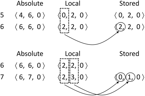
Figure 1. The setup of LAZ and LAX.

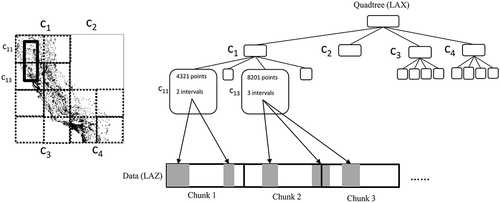
Figure 1 shows the typical setup of LAZ plus LAX. To solve a range query, the quadtree is traversed to determine the leaves that may have points in the queried region. Then, the relevant chunks are decompressed, and, finally, the resulting points are sequentially scanned to determine the points in the result. For example, in Figure 1 we want to retrieve the points within the region delimited by the rectangle with a thick solid line overlapping the quadrants $c_{11}$ and $c_{13}$. Observe that $c_{11}$ and $c_{13}$ are the quadrants on the left part of the bigger $C_1$, which contains four smaller quadrants that are surrounded by thick dotted lines. The search starts at the root of the quadtree following the quadrants overlapping the queried region. In this case, the search reaches the leaves corresponding to $c_{11}$ and $c_{13}$. As seen, $c_{11}$ contains 4321 points and 2 intervals. Each interval has an initial and a final position within the array storing the positions. In our example, since the two intervals are in the same chunk, only that chunk must be decompressed. In the case of $c_{13}$, it contains three intervals that are in chunks 2 and 3, thus both chunks must be completely decompressed to extract the points in the desired intervals.

The quadtree is limited to 2D space. Therefore, queries involving the third dimension are inefficient. In addition, there are no indexes for the attributes; thus, a sequential scan must be performed on the candidate points, making these queries inefficient as well. However, these queries are increasingly relevant because classification algorithms on point clouds may require the location of close points in the 3D space or nearby points in a 2D space with a given attribute value or range of values.

2.1.3. Scale factor and offset

LAS and LAZ store integer values. Therefore, the float numbers of real positions must be converted into positive integer values. For this purpose, LAS and LAZ use a scale factor and an offset for each dimension. The scale factor transforms a float value into an integer value. The offset is a value that moves the point cloud in the coordinate system to start at coordinate $⟨0,0,0⟩$. Both values, the scale factor and the offset, are represented as double floating values. Given a scale factor $s{f}_d$ and an offset $offse{t}_d$, the formula to calculate the corresponding position $p{{ }^{\mathrm{\prime }}}_d$ is: $p{{ }^{\mathrm{\prime }}}_d=(p_d-offse{t}_d)/s{f}_d$, where $p_d$ is the real coordinate in dimension $d$. For example, with $s{f}_d=0.1$ and $offse{t}_d=35.5$, the float value $p_d=35.8$ is converted to $p{{ }^{\mathrm{\prime }}}_d=(35.8-35.5)/0.1=0.3/0.1=3$. Likewise, the original values can be recovered as $p_d=(p{{ }^{\mathrm{\prime }}}_d\cdot s{f}_d)+offse{t}_d$. Isenburg (2013) shows that this strategy does not lose precision and thus it is a lossless representation. Moreover, this offers much more uniform precision than the corresponding floating-point value for the same number of bits. We will also use this strategy for representing the points in our proposal, using up to 64 bits for representing the integer coordinates.

2.2. Compact data structures

Compact data structures keep the data and the data structures around them in compressed form and provide the user with the capability of querying the data in compact form, that is, without decompressing them (Navarro 2016).

Most compact data structures are based on bitmaps or bitvectors. A bitmap is a bit array $B[1,n]$ that supports the following operations: i) $access(B,i)$, which returns the bit $B[i]$, for any $1\le i\le n$, ii) $ran{k}_b(B,p)$, which counts the number of occurrences of bit $b$ in bitmap $b$ until position $p$, and iii) $selec{t}_b(B,n)$, which returns the position of the $n$-th occurrence of bit $b$ in $b$. With bitmaps, we can simulate trees, graphs, grids, which are then used to enhance all sorts of complex data structures such as text indexes, spatial indexes, etc. (Navarro 2016). The target is not only to save space but provide several nice features. For instance, a tree represented with a bitmap does not use pointers, using less space for its representation, and, at the same time, can be as efficiently navigated as a pointer-based tree.

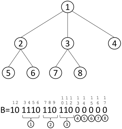
Figure 2 shows an example. The tree in the upper part is only represented with the bitmap $B$. By building rank and select structures on $B$, many operations can be done in constant time using only $B$. For example, it is possible to obtain the second child of the root node in constant time. Observe that the root node is represented by the bits at positions 3, 4, 5, and 6, and its first position is 3. The $t^{th}$ child of the node whose description starts at position $v$ can be computed as $child(v,t)=selec{t}_0(B,ran{k}_1(B,v-1+t))+1$, in our case $child(3,2)=selec{t}_0(B,ran{k}_1(B,4))+1=\text{break}selec{t}_0(B,3)+1=9+1=10$, that is, the description of the second child of the root node starts at position 10.

Figure 2. A tree represented with a bitmap.

The key factor to improve efficiency is that rank and select operations can be solved in constant time (see Munro (1996), for example), using $n+o(n)$ bits of total space. In practice, usually, rank is solved in constant time, whereas select is solved in $O(loglogn)$ time (Vigna 2008) with approximately 5% extra space over the original bitmap.

Several compact data structures have been developed for spatial data (Susana, Paramá, and Silva-Coira 2016; Ladra, Paramá, and Silva-Coira 2017; Pinto, Seco, and Gutierrez 2017; Brisaboa et al. 2020), but, until now, only for raster data.

2.3. Level-order unary degree sequence

Level-order unary degree sequence (LOUDS) (Jacobson 1989) is a compact data structure consisting in a level-wise representation of trees without pointers. In traditional tree representations, nodes are identified by the pointers to their position in memory. In a LOUDS representation, nodes are identified by their position in a bitmap. Therefore, using LOUDS, a tree is not physically implemented as a tree.

Given a tree $T$, the LOUDS representation is a bitmap $B$ where we first add bits 10. Then, we traverse $T$, starting at the root, level by level. For each node $v$ with $c$ children, $c$ 1-bits and one 0-bit are appended to $B$. These $c+1$ bits are the description of the node $v$. Figure 2 is a LOUDS representation of the tree in the upper part.

By building rank and select structures on $B$, we can perform several operations in constant time, among them, obtaining the parent, the $t^{th}$ child, the sibling, or the degree of a given node. For example, in Section 2.2, we show how to obtain the $t^{th}$ child of a given node.

If a tree $T$ has $n$ nodes, we need $n$ pointers for representing its topology, which typically require $nw$ bits, where $w$ is the machine word. Instead, using LOUDS, we only need $2n$ bits for the topology. To support rank and select operations in constant time, the total space rises to $3.6n$ bits, which can be decreased to $2.65n$ bits when using slower implementations of rank and select (Navarro 2016).

LOUDS trees can reduce the space considerably, but, for our case, it is even more important that a node $v$ is not identified by its position in memory (i.e. by a pointer) but by its position in the bitmap defining the tree. As we will explain later, this will be helpful for our proposal.

2.4. Quadtrees and octrees for representation or indexation

As we will see, our method uses an octree for binary matrices built applying the latest developments in the field of compact data structures, which we call a ${\mathrm{k}}^3-\mathrm{t}\mathrm{r}\mathrm{e}\mathrm{e}$. An octree is a quadtree for the 3D space. There are many variants of the quadtree (Samet 1984, 2006). We can roughly classify them into two groups, those mainly focused on compressing images (or rasters) and those focused on indexing data. The compression of images was its original target (Klinger 1971; Klinger and Dyer 1976), but many other works in this research line were later presented (Woodwark 1984; Lin 1997; Chan 2004; Chung, Liu, and Yan 2006; Zhang, You, and Gruenwald 2015; Graziosi et al. 2020).

The best-known quadtree-based method to index data consists in storing the leaves of a linear quadtree (Gargantini 1982) in a B+-tree (Abel and Smith 1983; Samet et al. 1984). Later, other indexes were also created based on quadtrees (Zhang and You 2010, 2013). As indexes, quadtrees were initially used to index black and white rasters (Corral, Vassilakopoulos, and Manolopoulos 1999) or point clouds (Finkel and Bentley 1974). We can say that those indexes only index the spatial component of the data, as they are only capable of finding white cells or points. In the case of rasters where cells can have more than two values, Zhang and You (2010) enrich the inner nodes of a quadtree with the min-max values of the region represented by such a node. This data structure, called Binned Min-Max Quadtree, is an index of the space and the values at cells.

The addition of the min-max values at the nodes improves the search performance. As in normal database management systems, if we want to search by two or more attributes at the same time, the ideal data structure is an index of those attributes combined. Having one index for each attribute may result in a slow response time, since the constraints on each attribute may be fulfilled by many records, and then to obtain the final solution, we have to run a costly intersection of all these records, whereas only a few records may fulfill all constraints on all attributes (Elmasri and Navathe 2016). Having the min-max values at nodes avoids the use of two different indexes, a spatial one and another indexing the values at cells. Instead, with this approach, we only have to run one search, and, at each step of the search process, we can prune the search both in space and values.

The quadtree-based indexes shown so far were auxiliary data structures to speed up searches over a different data structure where data are stored. The first data structure that combines raster (image) compression (and thus it can represent the data) and indexing capabilities was the compact data structure ${\mathrm{k}}^2-\mathrm{a}\mathrm{c}\mathrm{c}$ (De Bernardo et al. 2013; Brisaboa et al. 2020). It uses quadtrees represented with a similar strategy to that of LOUDS. Later, other works improved their results (Ladra, Paramá, and Silva-Coira 2017; Chow et al. 2020, 2022). Two are the main differences between this work and those previous methods. Those structures were designed for rasters, and each cell of the raster only has one value. The differences in this work are that, first, we aim at storing point clouds, and second, each point may have several attributes, instead of one value as in the case of rasters.

As a summary, the main difference with respect to the more traditional approaches is that while these works are either focused on representing the data using compression or on designing an auxiliary index of the data, our work combines these two worlds. Moreover, our data structure combines the index and the data, as most self-indexes of compact data structures, such as the case of the ${\mathrm{k}}^2-\mathrm{t}\mathrm{r}\mathrm{e}\mathrm{e}$ in the case of spatial data, and many other examples in other data types (Navarro 2016). Instead, the normal setup is to have an array-like data structure to store the data and an auxiliary tree to index the data. Moreover, our index is twofold as indexes the space and all the attributes of the points combined. Observe that the LAS/LAZ setup is the typical, that is, data are stored in an array structure, and an auxiliary index is built, which only indexes the space.

2.5. Compression of point clouds

As explained, much research effort was devoted to compressing images, which can be regarded as rasters or sometimes also called meshes (Peng, Kim, and Kuo 2005). However, we can also find works focused on compressing point clouds, but, as in the case of images, they are mainly focused on compressing the point cloud, but they do not care about querying the points either spatially or by any property of the points such as color (Ochotta and Saupe 2004).

Compression is achieved using kd-trees (Devillers and Gandoin 2000), octrees (Botsch, Wiratanaya, and Kobbelt 2002; Peng and Kuo 2003; Schnabel and Klein 2006), or different spatial transformations (Zhang, Florencio, and Loop 2014; De Queiroz and Chou 2016; Shuman et al. 2013; Fan, Huang, and Peng 2013). Some of these works were only focused on compressing the points, but later works also faced the compression of colors of the points (Yan, Jingliang Peng, and Gopi 2008; Zhang, Florencio, and Loop 2014; Chou, Koroteev, and Krivokuca 2020). Point cloud compressors use those transformations as a step that is combined with several other techniques, such as the RAHT coder (ISO/IEC JTC 1/SC 29/WG 7 2021). These techniques generally rely on a compression step where, in order to compress a given point, multiple neighbors are used to make a prediction that is somehow exploited by an entropy encoder. Recently, deep learning techniques have been also applied to improve different aspects of point cloud compression (Huang et al. 2020; Quach, Valenzise, and Dufaux 2020).

MPEG issued in 2017 a call for proposals for developing standards for point cloud compression (Liu et al. 2020; Graziosi et al. 2020). This effort already produced two standards: the geometry-based point cloud compression or G-PCC (ISO/IEC JTC 1/SC 29/WG 7 2021) and video-based point cloud compression or V-PCC (Schwarz et al. 2019).

However, all these techniques are strictly tied to image or video compression, where the main target is to render the image, and not to query certain regions of the space (Cao, Preda, and Zaharia 2019).

The main difference of our work with these proposals is that we are not focused on image compression capable of fast decompression (rendering), but on the ability to index and thus to search part of the point clouds, fulfilling constraints both in the spatial dimension and in the attribute value dimension.

2.6. ${\mathbf{k}}^2-\mathbf{t}\mathbf{r}\mathbf{e}\mathbf{e}$

The ${\mathrm{k}}^2-\mathrm{t}\mathrm{r}\mathrm{e}\mathrm{e}$ is a compact data structure initially designed to store and query web graphs (Brisaboa, Ladra, and Navarro 2014). However, it turns out to be a modern version of a region quadtree (Samet 2006). Indeed, since then, it has been used, among other purposes, as a spatial index (De Bernardo et al. 2013; Brisaboa et al. 2017; Silva-Coira et al. 2020; Brisaboa et al. 2019, 2021). In those works, the ${\mathrm{k}}^2-\mathrm{t}\mathrm{r}\mathrm{e}\mathrm{e}$ is used instead of a quadtree because it is more efficient in space and time since it is a pointerless representation of the quadtree equipped with efficient navigation through the tree. It is not a LOUD representation of a quadtree, but it is inspired in that representation.

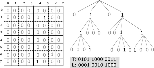
Given a binary matrix $M$ of size $n\times n$, and a parameter $k$, $M$ is divided into $k^2$ submatrices of size $n/k^2\times n/k^2$. For each of those submatrices, a child node is added to the root node. Each node only contains a bit: 0 indicates that the submatrix is full of 0-bits and 1 means that the submatrix contains at least one 1-bit. Now, for each of the submatrices with at least one 1-bit, the process continues recursively. The resulting tree is stored as a bitmap following a breadth-first traversal of the tree nodes. The ${\mathrm{k}}^2-\mathrm{t}\mathrm{r}\mathrm{e}\mathrm{e}$ divides that bitmap in two: $L$, which is formed by the bits corresponding to the last level of the tree, and $T$, which contains the rest. The reason is that, in $L$, it is not necessary to build rank structures, since that level is never navigated, whereas in $T$ it is necessary.

Figure 3 shows an example. The ${\mathrm{k}}^2-\mathrm{t}\mathrm{r}\mathrm{e}\mathrm{e}$ can efficiently answer several queries, like retrieving the value of a single cell, row/column queries, or spatial range queries. All of them require navigating the tree, which is a very fast process, since it is based on rank and select operations, which are constant-time operations. Given a 1-bit at position $p$ in $T$, that is, a node with children, these children are sequentially located at positions $children(p)=\{ran{k}_1(T,p)\cdot k^2,\dots ,ran{k}_1(T,p)\cdot k^2+k^2-1\}$ of $T:L$. The parent of a node at position $p$ of $T:L$ is computed as $parent(p)=selec{t}_1(T,p/k^2)$. Of course, navigating a pointer-based tree requires also constant time operations. However the ${\mathrm{k}}^2-\mathrm{t}\mathrm{r}\mathrm{e}\mathrm{e}$ has been shown 2–3 times faster than a traditional quadtree (Brisaboa et al. 2020).

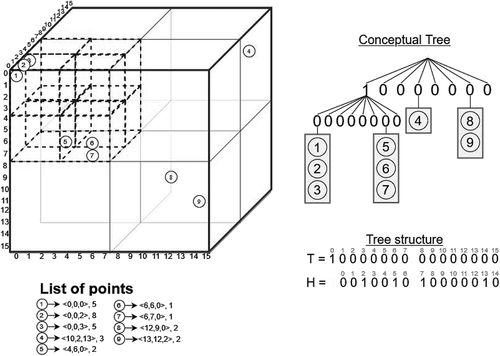
Figure 3. A binary raster, the conceptual tree, and the corresponding ${\mathrm{k}}^2-\mathrm{t}\mathrm{r}\mathrm{e}\mathrm{e}$, with $k=2$.

2.7. ${\mathbf{k}}^{\mathbf{3}}-\mathbf{t}\mathbf{r}\mathbf{e}\mathbf{e}$

The ${\mathrm{k}}^3-\mathrm{t}\mathrm{r}\mathrm{e}\mathrm{e}$ (De Bernardo et al. 2013) is the 3D version of the ${\mathrm{k}}^2-\mathrm{t}\mathrm{r}\mathrm{e}\mathrm{e}$. As the ${\mathrm{k}}^2-\mathrm{t}\mathrm{r}\mathrm{e}\mathrm{e}$, which is a modern region quadtree, the ${\mathrm{k}}^3-\mathrm{t}\mathrm{r}\mathrm{e}\mathrm{e}$ is a modern octree (Meagher 1982) (a 3D quadtree). Figure 4 shows an example, including a three-dimensional binary matrix, its conceptual tree, and its representation, which is the ${\mathrm{k}}^3-\mathrm{t}\mathrm{r}\mathrm{e}\mathrm{e}$ (bitmaps $T$ and $L$). The ${\mathrm{k}}^3-\mathrm{t}\mathrm{r}\mathrm{e}\mathrm{e}$ can be efficiently navigated using the same procedures as those for ${\mathrm{k}}^2-\mathrm{t}\mathrm{r}\mathrm{e}\mathrm{e}$, but extended to three dimensions.

Figure 4. A sequence of binary rasters and the corresponding ${\mathrm{k}}^3-\mathrm{t}\mathrm{r}\mathrm{e}\mathrm{e}$.

Given that if a node has children, then it has exactly $k^3$ children, we do not need to mark the end of the children of one node. Therefore, the ${\mathrm{k}}^3-\mathrm{t}\mathrm{r}\mathrm{e}\mathrm{e}$ of a tree of $n$ nodes uses exactly $n$ bits to represent the topology. Thus, after adding the rank and select structures, it needs between $1.65n$ bits and $2.6n$ bits.

Therefore, the use of a LOUDS-based approach to represent an octree produces two benefits. First, a save in space, from the $w$ bits per node of a traditional octree to the $1.65-2.6$ bits per node. Second, each node $v$ is not identified by its pointer, but by its position in $T$ or $L$. This property will allow us to index the different attributes of a point without having to place the information in the node of the octree. We will explain this later.

2.8. DACs

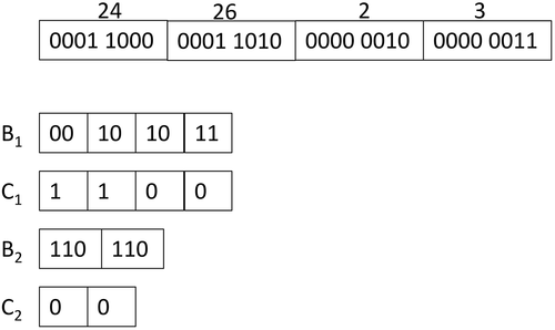
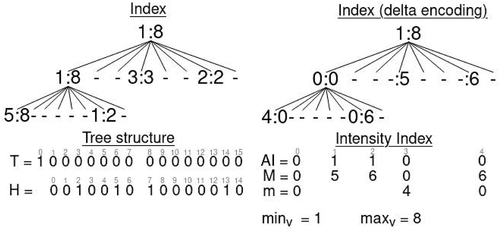
Directly Addressable Codes (DACs) (Brisaboa, Ladra, and Navarro 2013) consist in a compact data structure for sequences of integers, which not only compresses the sequence but, at the same time, supports the retrieval of any given integer of the sequence without the need to decompress the preceding integers. DACs obtain compression if the sequence of integers has a skewed frequency distribution toward smaller integer values.

Given a sequence of integers $X$ = $x_1,x_2,\dots ,x_n$, DACs take the binary representation of each number and divide it into buckets that are stored as a level-shaped structure as follows. The first level is formed by a bitmap $B_1$ that contains the first (least significant) $n_1$ bits of the binary representation of each integer. $B_1$ has an associated bitmap $C_1$ to indicate whether the binary representation of each integer requires more than $n_1$ bits (1) or not (0). In the second level, the bitmap $B_2$ stores the next $n_2$ bits of the integers with a value of 1 in $B_1$. The associated bitmap $C_2$ signals the integers that need more than $n_1+n_2$ bits, and so on. This process is repeated for as many levels as needed. The number of levels $\mathrm{\ell }$ and the number of bits of the buckets are calculated in order to maximize compression. Each value $x_i$ is retrieved using $rank$ operations on the bitmaps $C_l$ and extracting the corresponding chunks of the arrays $B_l$.

In Figure 5, we can see a sequence of 8-bits integers and its corresponding representation using DACs. Integers 2 and 3 are represented with three bits, and numbers 24 and 26 are represented using seven bits. As seen, if numbers are small, compression is achieved. That is, instead of using $w$ bits per integer, DACs try to approach the optimal $log(n)$ bits per integer by using a clever algorithm to determine the bucket sizes.

Figure 5. An example of DACs. At the top part of the figure, we show the sequence of integers $X=24,26,2,3$. At the bottom part of the figure, we show the DACs representation using a level-shaped data structure.

3. Our proposal: ${\mathbf{k}}^{\mathbf{3}}-\mathbf{l}\mathbf{i}\mathbf{d}\mathbf{a}\mathbf{r}$

In this section, we present a new compact data structure, called ${\mathrm{k}}^3-\mathrm{l}\mathrm{i}\mathrm{d}\mathrm{a}\mathrm{r}$, which represents a cloud of LiDAR points in compressed space and also contains an index to perform efficient queries over the data. In this work, we assume that the set of points is represented in Point Data Record Format 0 of LAS Specification 1.4 (The American Society for Photogrammetry and Remote Sensing 2019). We are using the attributes defined by this standard, but our structure can be adapted to support other different formats. Section 2.1.3 gives some details on the conversion of coordinates from real values to positive integer values, which is also used by LAS.

In Section 3.1, we show the conceptual description of our structure. Section 3.2 lists the structures used to represent the ${\mathrm{k}}^3-\mathrm{l}\mathrm{i}\mathrm{d}\mathrm{a}\mathrm{r}$. Then, in Section 3.3, the construction algorithm is explained. Finally, Section 3.4 describes the three queries implemented in this work.

3.1. Conceptual description

Let $C$ be an input three-dimensional matrix, or cube, of size $n\times n\times n$ that stores a set of LiDAR points.² A LiDAR point is composed of three coordinates ($x$, $y$, and $z$) and a set of attributes, like the intensity, scan direction, number of returns, etc.

Our structure follows a similar strategy to that used by the ${\mathrm{k}}^3-\mathrm{t}\mathrm{r}\mathrm{e}\mathrm{e}$ but adapted to store LiDAR points and not only to indicate in which cells there are points. Moreover, we need some additional structures to store the values of the attributes of the points.

The ${\mathrm{k}}^3-\mathrm{l}\mathrm{i}\mathrm{d}\mathrm{a}\mathrm{r}$ performs a recursive subdivision of the 3D cube $C$ and builds the tree representation of that subdivision in a similar way as the ${\mathrm{k}}^3-\mathrm{t}\mathrm{r}\mathrm{e}\mathrm{e}$. However, unlike the original ${\mathrm{k}}^3-\mathrm{t}\mathrm{r}\mathrm{e}\mathrm{e}$, the division process stops in three different cases: when it reaches the tree depth; if the subcube is empty (i.e. it does not contain any points); and when the processed subcube contains fewer points than a defined threshold $l$, which is a common stop condition in octree segmentation (Elseberg, Borrmann, and Nuchter 2011) of the tree is empty or contains a set of LiDAR points. By navigating the tree, a specific point or set of points can be efficiently retrieved.

In order to store the attributes of each point, we use different compact data structures depending on the value type of each attribute. These structures must include direct access to any position of the array in an efficient way. Therefore, we can easily obtain the attributes of a specific point.

3.2. Data structures

We use different data structures to store the conceptual tree:

• Tree structure (bitmap $T$): The topology of the tree is represented using the structure $T$. $T$ is a bitmap that indicates when a node has children or not (that is, it is a leaf). Therefore, we set a 1 if the node has children (i.e. it is divided into subcubes) and a 0 when the corresponding cube is empty or its number of points does not exceed the threshold $l$. Unlike the ${\mathrm{k}}^3-\mathrm{t}\mathrm{r}\mathrm{e}\mathrm{e}$, our structure does not need to represent the last level of the tree (bitmap $l$ in the ${\mathrm{k}}^3-\mathrm{t}\mathrm{r}\mathrm{e}\mathrm{e}$) since other structures (bitmaps $H$ and $N$), shown below, are responsible for representing the leaves.

• Leaf nodes (bitmap $H$): The structure $H$ is a bitmap that contains a bit for each 0 in $T$, i.e. when a node is leaf. Thus, $|H|=ran{k}_0(T,|T|)$. This bitmap differentiates empty subcubes from those that contain fewer points than the threshold $l$, both marked as 0s in $T$. Hence, for a node $i$ such that $T[i]=0$, we set $H[ran{k}_0(T,i-1)]\leftarrow 1$ when the corresponding subcube contains a set of points, and a 0 when the node is empty.

• Number of points (bitmap $N$): The bitmap $N$ stores the number of points of each non-empty leaf, i.e. when $H[ran{k}_0(T,i-1)]=1$, being $i$ the position of the node in $T$. These values are represented using unary code. If a node has $v$ points, we set $0^{v-1}$-bits and one 1-bit in the bitmap $N$. This means that each point in the cloud is represented with a bit in $N$, where the 1 marks the last point of the subcube. For a non-empty leaf node where $H[i]=1$ and $e=ran{k}_1(H,i-1)$ (number of not-empty nodes before position $i$), we can calculate first and last positions of its points in $N$ as $selec{t}_1(N,e)+1$ and $selec{t}_1(N,e+1)$, respectively.

• Coordinates: Let us consider a point with absolute coordinates $(x,y,z)$ and let us suppose that it is located in a subcube corresponding to a leaf of size $s\times s\times s$. To represent it, we store the tuple $⟨x{ }^{\mathrm{\prime }},y{ }^{\mathrm{\prime }},z{ }^{\mathrm{\prime }}⟩=⟨xmods,ymods,zmods⟩$. With this, we reduce the magnitude of the values, and thus we can use fewer bits to represent them. Observe that we can easily recover their original values descending through the tree.

We use two different strategies to store the coordinates of the points.

1. Three arrays of coordinates ($X$, $Y$, and $Z$): The first option is to store each component of each point in the corresponding array. The three arrays are encoded with DACs.

2. Array of coordinates (P): The second option only uses one array to represent the three coordinates of a point. Each point of a node is encoded as a unique value computed as $x\cdot s^2+y\cdot s+z$, where $s$ is the size of the corresponding subcube of the node. This array is also encoded with the compact data structure DACs.

In both cases, points that belong to the same node are sorted following a row-major order. That is, they are ordered first by the X coordinate, then by the Y coordinate, and finally by the Z coordinate. These arrays are aligned with bitmap $N$. Once we know the range of positions of $N$ we are interested in, the same positions in $X$, $Y$, $Z$ (or $P$) contain the desired coordinates.

• Attributes: We have one structure for each attribute. Depending on the type of attribute, we use integer arrays (for intensity, scan angle, return number, etc.) or bitmaps when we only need a single bit per value (as the scan direction and edge). The arrays of integers are encoded with DACs. Again, these arrays are aligned with bitmap $N$.

In order to return a point at position whose position in $N$ is $p$, we access $X[p]$, $Y[p]$, $Z[p]$ (or $P[p]$ if we are using the second strategy) and $intensity[p]$, $scan\mathrm{\_}angle[p]$, and so on.

3.3. Construction

The construction process starts by dividing the cube $C$ into $k^3$ equal-sized subcubes. From the root of the tree, a child node is appended for each subcube. The algorithm then continues through each child node. If it does not contain any points, the process stops for that branch, adds a 0-bit to bitmap $T$, and continues with the next node. When the number of points is less than the threshold $l$, the process also stops for that branch, adding again a 0-bit to bitmap $T$, the number of points is encoded in bitmap $N$, and the list of points associated with that node is represented in the array(s) of coordinates ($X,Y,Z$ or $P$). Otherwise, a 1-bit is added to bitmap $T$, the node is again divided into $k^3$ subcubes and the previous process is repeated until reaching leaf nodes.

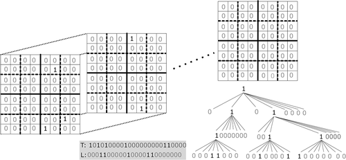
Let us explain the algorithm with an example. Figure 6 (upper-left) contains a cloud of LiDAR points in a space of size $16\times 16\times 16$. The list of points is shown in the bottom left of the figure, where each one is represented as a circle with a unique identifier, a set of coordinates $⟨x,y,z⟩$, and the intensity value. To simplify the explanation, we have only taken into account the intensity attribute but the process is the same for the rest of the attributes. In this example, the scale factor is 1 and the offset is 0 for the three dimensions (transformation is not applied to the input data). Additionally, we are using a value of $k=2$ and the threshold to stop dividing is $l=4$. The conceptual tree representation of the ${\mathrm{k}}^3-\mathrm{l}\mathrm{i}\mathrm{d}\mathrm{a}\mathrm{r}$ is shown in the upper right part of the figure.

Figure 6. Example of LiDAR point cloud and its representation using ${\mathrm{k}}^3-\mathrm{l}\mathrm{i}\mathrm{d}\mathrm{a}\mathrm{r}$. We only show here the data structures needed for representing the tree structure, using $k=2$ and threshold $l=4$. A point (circle) is represented by a unique number and it has associated three coordinates and an intensity value. For example, point 5 is located at coordinates $⟨4,6,0⟩$ and has an intensity value of 2.

In this example, from the eight subcubes of size $8\times 8\times 8$, only the one that contains points 1–7 is divided into subcubes of size $4\times 4\times 4$, since it contains more points than threshold $l=4$. This is reflected in the conceptual tree, where only the first child has a 1-bit to signal this. The four $4\times 4\times 4$ subcubes are not further divided, and thus all their bits in the second level of the tree have a 0-bit.

$T$ is simply the levelwise traversal of the conceptual tree. $H$ has a bit for each 0-bit in $T$. In the figure, we aligned the bits of $H$ with the corresponding 0-bit of $T$, but observe that they are not really aligned, since $H$ does not have bits for the 1-bits of $T$. This is done to save space. To recover the alignment between the 0-bits in $T$ and their corresponding bits in $H$, we have to use rank operations, as previously explained.

Figure 7 shows how the LiDAR points are stored in our structure. Recall that points belonging to the same node are sorted following a row-major order. They are representing following a level-wise traversal of the tree; thus, we start with the fourth node at the first level of the tree. This node only contains point 4. First, we append the number of points in the bitmap $N$ in unary, in this case, $1$ (1 in unary). Next, we calculate the local coordinates of the point, whose absolute coordinates are $⟨10,2,13⟩$. Notice that the subcube has size $8\times 8\times 8$, therefore, $x=10mod8=2$, $x=2mod8=2$, and $z=13mod8=5$. Hence, the point $⟨10,2,13⟩$ becomes $⟨2,2,5⟩$ and it is stored as $X[0]\leftarrow 2$, $Y[0]\leftarrow 2$, and $Z[0]\leftarrow 5$. We continue with the rest of the nodes, following a breadth-first order of the tree. In this example, with the seventh node of the first level and then with the first and seventh nodes of the next level.

Figure 7. Representation of the LiDAR points of the running example using the ${\mathrm{k}}^3-\mathrm{l}\mathrm{i}\mathrm{d}\mathrm{a}\mathrm{r}$, including bitmap $N$ and the coordinates and attribute arrays.

For a set of points that belong to the same node, we use some optimizations to make the values smaller. The coordinates of a point $p_n=⟨v{1}_n,v{2}_n,v{3}_n⟩$ are stored using delta encoding with respect to the previous point $p_{n-1}=⟨v{1}_{n-1},v{2}_{n-1},v{3}_{n-1}⟩$ as $vi{{ }^{\mathrm{\prime }}}_n=v{i}_n-v{i}_{n-1}$ iff $v{e}_n=v{e}_{n-1}$ for $1<=e<i-1$. The target is to take advantage of the compression achieved by DACs. As seen in Section 2.8, DACs try to come closer to using $log(n)$ bits for an integer $n$, so by reducing the magnitude of the numbers, we obtain better compression.

We are going to explain this using the seventh node at the second level. This node contains points 5, 6, and 7. Observe in Figure 8 in the upper part the encoding of the points 5 and 6. Their absolute coordinates are $⟨4,6,0⟩$ and $⟨6,6,0⟩$ that after applying modulo 4 became $⟨0,2,0⟩$ and $⟨2,2,0⟩$. The first point of the leaf is stored with its local coordinates. For the second (point 6), the $x$ coordinate is delta encoded, and it is highlighted with a box with dotted points. However, as soon as the box with dotted points has two different numbers, the next coordinates are not delta encoded. In this case, the $x$ values of points 5 and 6 are different, and thus, the $y$ and $z$ coordinates are not delta encoded.

Figure 8. Example of delta encoding of points.

In the lower part, we can see how the point 7 is stored. The $x$ coordinate as always is delta encoded, and as it has the same value (2) in both points, the $y$ coordinate is also delta encoded. However, the $y$ coordinate has different values in point 6 (2) and point 7 (3), and thus the $z$ coordinate is not delta encoded.

Finally, the intensity values are stored in the array $I$ following the same order as their points. In case of having more attributes, a sequence $A$ is created for each one.

According to the classification of point compressors seen in Section 2.1.1, ${\mathrm{k}}^3-\mathrm{l}\mathrm{i}\mathrm{d}\mathrm{a}\mathrm{r}$ is a lossless, non-progressive, non-streaming, point-permuting compressor. The non-streaming property means that it needs to have all points before compression starts, thus its memory footprint is bigger. This is a common property of compact data structures. Since main memory is currently cheaper than in the time where the disk-based applications were mandatory, and as long as the data can fit in main memory, it is worthwhile to get rid of disk accesses. It is a point-permuting compressor, as all compressors based on a octree. However, unlike LAZ, which is not really a random-access compressor, ${\mathrm{k}}^3-\mathrm{l}\mathrm{i}\mathrm{d}\mathrm{a}\mathrm{r}$ is a truly random-access compressor.

3.3.1. Storing coordinates in a unique array $P$

We have implemented an alternative to store the coordinate in a unique array instead of three different structures. With this second option, the local coordinates are represented using a single value. For example, we store point 4, with local coordinate $⟨2,2,5⟩$, as $P[0]=x\cdot s^2+y\cdot s+z=2\cdot 64+2\cdot 8\text{break}+5=149$, where $s$ is the size of the current subcube. We repeat the process for the rest of the points. Moreover, we apply a delta encoding to points of the same node. For example, we represent the point $p_5=⟨2,0,0⟩$ as $p_5=2\cdot 16+0\cdot 4+0=32$, the point $p_6=⟨3,1,0⟩$ as $p_6=3\cdot 16+1\cdot 4+0=52$, and the point $p_7=⟨3,2,0⟩$ as $p_6=3\cdot 4\cdot 4\text{break}+2\cdot 4+0=56$. Then, we use delta encoding for these values, therefore we set $P[6]\leftarrow 32$, $P[7]\leftarrow p_6-p_5=52-32=20$, and $P[7]\leftarrow p_7-p_6\text{break}=56-52=4$

3.4. Supported queries

In this section, we describe three queries implemented for the ${\mathrm{k}}^3-\mathrm{l}\mathrm{i}\mathrm{d}\mathrm{a}\mathrm{r}$. These queries are common in multi-dimensional environments.

3.4.1. Obtaining all points in a region (getRegion)

This query obtains all points inside a region defined by $⟨x_i,y_i,z_i⟩$ $\times$ $⟨x_e,y_e,z_e⟩$.³ The ${\mathrm{k}}^3-\mathrm{l}\mathrm{i}\mathrm{d}\mathrm{a}\mathrm{r}$ performs a top-down traversal of the tree, following the nodes corresponding to subcubes that overlap with the region of interest. When the process reaches a leaf node, the coordinates of each point are obtained and checked. For those points that belong to the region of interest, their attributes are also retrieved and attached to the final result. In this step, our algorithm is able to reduce the number of points checked using some mechanisms. Recall that points follow a row-major order, for example, when the algorithm reaches a point $⟨x,y,z⟩$ and $x>x_e$, the process stops because there are no more valid points in the current leaf node. In addition, the value of coordinate $y$ is only retrieved when $x_i\le x<x_e$ and analogous for the value of coordinate $z$.

The pseudocode of this query is shown in Algorithm 1, which is a recursive procedure. Let $n\times n\times n$ be the size of the space and $H$, $N$, $X$, $Y$, and $Z$ global parameters. The precalculated value $1s\mathrm{\_}in\mathrm{\_}T$ is the total number of 1s in bitmap T. In order to obtain all the points contained within a region $⟨x_i,y_i,z_i⟩\times ⟨x_e,y_e,z_e⟩$, the first call of the algorithm is invoked as $\mathbf{g}\mathbf{e}\mathbf{t}\mathbf{R}\mathbf{e}\mathbf{g}\mathbf{i}\mathbf{o}\mathbf{n}(n,x_i,y_i,z_i,x_e,y_e,z_e,0)$. Parameter $result$ stores the list of points returned by this procedure.

Lines 1–3 determine which subcubes overlap the queried region, that is, which nodes have to be inspected to find the result. Line 4 obtains the position in $T$ of each subcube by using children_pos, which indicates the position of the first child of the node. The condition in line 5 determines if the node is at the maximum level $lo{g}_{k}n$ of the tree or at an intermediate level.

Next, line 6 indicates whether the current node is a leaf or an internal node. Lines 7–10, which are executed in the second case, compute first the local positions of the region, that is, determine the portion of the region that overlaps the current subcube, and then recursively invoke the function with those values (line 10). The position of its children in bitmap $T$ is calculated as $ran{k}_1(T,pos)\cdot k^3$, and the size of the subcube is $s/k$.

Lines 12–22 are executed in the case of reaching a leaf node. In line 12, variable $\mathrm{\#}leaves$ counts the number of leaves (0s in $T$) until position $pos$. Next, line 13 checks if the current node is empty; otherwise, the algorithm calculates the initial and final position of the points in $N$. For that, line 14 counts the number of non-empty leaves (represented by a 1 in $H$) up to the current position (variable $\mathrm{\#}ones$). Lines 15–18 get the first and last positions in arrays $X$, $Y$, and $Z$ using the operations $selec{t}_1(N,\mathrm{\#}ones)+1$ and $selec{t}_1(N,\mathrm{\#}ones+1)$, respectively. All intermediate bits belong to the current node and are associated with a point. Finally, lines 18–22 return the coordinates of each point and check if it is within the queried region. Those that meet the condition are added to the result together with the values of their attributes.

Lines 24–32 are only executed when the algorithm reaches the tree depth, i.e. level $lo{g}_{k}n$. Observe that several points can have the same coordinates. This level is not represented in $T$; therefore, the position in $H$ is calculated as $\mathrm{\#}leaves\leftarrow pos-1s\mathrm{\_}in\mathrm{\_}T$ (line 24). Lines 25–32 are equal to lines 13–22 except that the algorithm does not need to calculate the local positions or check if they are within the region.

Algorithm 1: getRegion

$(s,x_i,y_i,z_i,x_e,y_e,z_e,children\mathrm{\_}pos)$ returns all LIDAR points from region $⟨x_i,y_i,z_i⟩$ $\times$ $⟨x_e,y_e,z_e⟩$

Figure 9 shows an example of this operation. We want to retrieve the points in the cube $[⟨2,2,0⟩\times ⟨3,5,0⟩]$, which is the shaded region in Figure 9(b).

Figure 9. Example of getRegion.

The operation is launched with getRegion(8,2,2,0,3,5,0,0). Lines 1–3 determine which subcubes of size $4\times 4\times 4$ overlap the queried region, which, in this case, are the subcubes $c_1$ and $c_3$. These two subcubes are highlighted in the space of the figure with thick lines. The fors of lines 1–3 process those subcubes one by one. For $c_1$, line 4 computes its position in $T$, which is $pos=0$ (see that position highlighted in Figure 9(c).

Since we are not at the last level of the tree (line 5), the flow reaches line 6. Since $T[0]=1$, lines 7–9 obtain the relative coordinates of the part of the queried region overlapping $c_1$. This is $[⟨2,2,0⟩\times ⟨3,3,0⟩]$, using relative coordinates within $c_1$, which is the region with vertical stripes in the space. Then, a new call getRegion(4,2,2,0,3,3,0,8) is issued, since $rank(T,0)\cdot k^3=8$, that is, the position of the first child of $c_1$ in $T$.

The call getRegion(4,2,2,0,3,3,0,8) processes $c_1$. Lines 1–4 determine which subcubes of size $2\times 2\times 2$ of $c_1$ overlap the queried region, which, in this case, is only subcube $c_{14}$, which is highlighted with thick dotted lines in Figure 9(b). Line 4 obtains the position in $T$ corresponding to $c_{14}$, which is $pos=11$. Observe that that bit corresponds to the node with vertical stripes in the last level of the conceptual tree. The check of line 5 takes the flow to line 6, and, since $T[11]=0$, the flow jumps to line 12. This line obtains the bit in $H$ corresponding to the current leaf. Observe that we are processing the subcube $c_{14}$ whose bit in $T$ is at position 11, but, as seen in the figure, its corresponding bit in $H$ is at position $\mathrm{\#}leaves=8$. We aligned them in the figure to facilitate the understanding, but observe that the positions are not the same for aligned bits.

As explained, in line 13, it is checked whether the subcube has points by accessing $H[8]$. Since it stores a 1-bit, the flow reaches line 14. Lines 14–17 compute the positions in bitmaps $X$, $Y$, and $Z$ of the coordinates of the points within $c_{14}$. For this, the algorithm has to detect in $N$ the positions corresponding to the position 8 of $H$. Line 14 counts the number of 1-bits in $H$ until position $ran{k}_1(H,8-1)=1$. Then, line 16 obtains the desired position as $selec{t}_1(N,1)+1=1$, that is, the first bit in $N$ corresponding to $c_{14}$ is at that position. Then, the algorithm checks that position and the contiguous until reaching a 1-bit, each 0-bit means that a second, third, etc., point is present in the same cube, however since the position 1 of $N$ already has a 1-bit, then $c_{14}$ only contains one point, and its coordinates are at position 1 of $X$, $Y$, and $Z$.

Line 19 obtains the coordinates in the full space. Observe that from $X$, $Y$, and $Z$, we obtain the point $⟨0,1,0⟩$, but those are relative coordinates within $c_{14}$, the call to calculateCoord returns the absolute coordinates $⟨2,3,0⟩$. Line 19 checks if that point is within the queried region, and as in this case this is true, the point is reported as a result, and then this ends this recursive call.

Now, the flow returns to the first call getRegion(8,2,2,0,5,3,0,0) to process the second subcube of size $4\times 4\times 4$ overlapping with the queried region, that is $c_3$. Line 4 computes its position in $T$, which is $pos=2$ (see its position highlighted in $T$). Next, line 10 issues getRegion(4,4,4,0,5,5,0,24), since $rank(T,2)\cdot k^3=24$, this is the position in $T$ of the first child of $c_3$.

Lines 1–4 determine that the only subcube of size $2\times 2\times 2$ of $c_3$ that overlaps the queried region is $c_{32}$. Line 4 obtains the position $pos=25$ in $T$ corresponding to $c_{32}$. The bit in $H$ corresponding to $c_{32}$ is computed in line 12, which obtains $\mathrm{\#}leaves=22$. Since $H[22]=1$, $c_{32}$ has points. Lines 14–17 determine that it has two points, since as it is highlighted in Figure 9(c), the position in $N$ corresponding to position 22 of $H$, that is position 5, has a 0-bit and position 6 a 1-bit. Then, in position 5 and 6 of $X$, $Y$, and $Z$, we can obtain the coordinates of those points.

3.4.2. Obtaining all points of a two-dimension region (getRegionxy)

For a region $⟨x_i,y_i⟩$ $\times$ $⟨x_e,y_e⟩$, this query obtains the set of points that belong to the region of interest. This query is a straightforward extension of the query getRegion but without taking into account the coordinate of the $z$ dimension.

3.4.3. Obtaining all points of a region filtered by attribute value (filterAttregion)

This query returns all points contained in a region $⟨x_i,y_i,z_i⟩$ $\times$ $⟨x_e,y_e,z_e⟩$ with the value of attribute A within a range $[A_i,A_e]$. The algorithm also performs a top-down traversal of the tree adding the points that meet the conditions. Unlike the query getRegion, when the process reaches a leaf node, the attribute value is obtained and compared to the given range $[A_i,A_e]$ after checking the coordinates of the point. The rest of the attributes are only retrieved if the point belongs to the region of interest and the attribute value is within the range.

4. Adding attribute indexes: ${\mathbf{k}}_{\mathbf{i}}^{\mathbf{3}}-\mathbf{l}\mathbf{i}\mathbf{d}\mathbf{a}\mathbf{r}$

This section introduces a new version of ${\mathrm{k}}^3-\mathrm{l}\mathrm{i}\mathrm{d}\mathrm{a}\mathrm{r}$, denoted ${\mathrm{k}}_{\mathrm{i}}^3-\mathrm{l}\mathrm{i}\mathrm{d}\mathrm{a}\mathrm{r}$, which includes an index to prune points using the values of attributes during a top-down traversal of the tree. This indexation is not provided by an additional index/tree, but it is included in the same tree used by the normal ${\mathrm{k}}^3-\mathrm{l}\mathrm{i}\mathrm{d}\mathrm{a}\mathrm{r}$. This allows the pruning of all dimensions (space and attribute values) at each step of the search.

The basic idea is to store at each node of the tree the minimum and maximum values of the indexed attribute of the points it contains. Although this section is explained for a single attribute, our structure can be expanded to include multiple indexes on different attributes following the same procedure.

In Section 4.1, we explain the new structures to represent the index in the ${\mathrm{k}}_{\mathrm{i}}^3-\mathrm{l}\mathrm{i}\mathrm{d}\mathrm{a}\mathrm{r}$ version. Moreover, Section 4.2 gives details of the construction of this variant. Finally, Section 4.3 shows how the navigation varies concerning the original version presented in Section 3.4.3.

4.1. Data structures to represent the index

In addition to the structures explained in Section 3.2, the following are used to represent the index on an attribute:

• Index tree (bitmap $AI$): The topology of the index is represented with a bitmap $AI$. For each non-empty node, we set a 1 when all points of the node have the same value in the attribute, that is, the minimum and maximum values are equal, and a 0 in other case. Given a node $i$ with $T[i]=1$ or $H[ran{k}_0(T,i-1)]=1$, the corresponding node in the index is calculated as $AI[ran{k}_1(T,i)+ran{k}_1(H,ran{k}_0(T,i-1))-1]$. For instance, in Figure 10, the corresponding position of the first node at the second level (position 8 in T) is calculated as $AI[ran{k}_1(T,8)+ran{k}_1(H,ran{k}_0(T,8-1))-1]=AI[ran{k}_1(T,8)\text{break}+ran{k}_1(H,7))-1]=AI[1+3-1]=AI[3]$

Figure 10. Conceptual tree and structures of ${\mathrm{k}}_{\mathrm{i}}^3-\mathrm{l}\mathrm{i}\mathrm{d}\mathrm{a}\mathrm{r}$ that represent the index of intensity attribute. Bitmaps $T$ and $H$ are not part of the attribute index, they correspond to the tree topology that are already part of ${\mathrm{k}}_{\mathrm{i}}^3-\mathrm{l}\mathrm{i}\mathrm{d}\mathrm{a}\mathrm{r}$ data structure, as shown in Figure 6. In the conceptual tree of the attribute index, each node shows the minimum and maximum intensities of their points as $m:M$. The ${\mathrm{k}}_{\mathrm{i}}^3-\mathrm{l}\mathrm{i}\mathrm{d}\mathrm{a}\mathrm{r}$ adds arrays $AI$, $M$ and $M$ for speeding up queries on that attribute.

• Minimum and maximum values (arrays $m$ and $m$): We use two different arrays, $m$ and $m$ to represent the minimum and maximum values, respectively. Observe that if $AI[i]=1$, both values are equal. Therefore, we only save the minimum value in $m$ when it is different from the maximum value. We can easily access the minimum of a node when $AI[a]=0$ with the formula $m[ran{k}_0(AI,a-1)]$. In order to obtain smaller numbers, and thus, as explained in Section 2.8, DACs can represent them with fewer bits, our structure stores the values of a node as the difference with respect to the corresponding parent. Finally, both arrays are encoded using the compact data structure DACs, and the global maximum and minimum values of the cube are stored in $ma{x}_v$ and $mi{n}_v$. Following the previous example, where $AI[3]=0$ and the minimum and maximum value of the parent node are 1 and 8, respectively, the maximum is calculated as $max\leftarrow ma{x}_v-M[3]=8-0=8$ and the minimum as $min\text{leftarrowm}[ran{k}_0(AI,3-1)]+mi{n}_v=m[1]+1=4\text{break}+1=5$.

As explained, our method combines in one data structure the data, an index of the space, and now, an index for each attribute. We describe the case of a single integer attribute. This setup is more efficient than that of a traditional configuration, where the index or indexes are separate data structures. To perform multikey searches (i.e. searches involving constraints on several attributes), it is better to have a single index for all indexed elements. In the literature, there are several methods to address this issue such as a grid file (Sevcik and Hinterberger 1984) or a partitioned hash (Burkhard 1976). However, in current database management systems, this issue is solved with an ordered index on multiple attributes (Elmasri and Navathe 2016, Sect 17.4.1) using as keys of the $B^{+}$-tree the concatenation of the values of all indexed attributes. We can use the same idea for our case, extending the idea of the Binned Min-Max Quadtrees, to have a pair of min-max values in each node of the octree for each indexed attribute. For each node of the octree, this approach requires the $w$ bits of the pointer to the node and another $2w$ bits per indexed attribute, that is, $(2a+1)w$ bits, being $a$ the number of attributes. Observe that we cannot compress these min-max values at the nodes of the octree, since they are concatenated, and to be able to access a given pair, they must be fixed in length. To this, we have to add the pointers to the data file storing the data themselves. As explained, LAS index stores for each leaf of the quadtree one or more intervals. Each of these intervals is encoded by using two positions of the data file where are placed the points corresponding to the leaf, that is $2w$ bits per interval. We cannot bound the number of intervals at each leaf but assuming a quadtree with $v$ nodes of which $l$ are leaves, we need at least $v(2a+1)w+2lw$ bits. Instead, our method gets rid of pointers, so this is $vw+2lw$ less bits. In addition, instead of using $2w$ bits per min-max pair at each node, since we are able to detach those values from the nodes of the tree, we can compress them with DACs, which use a variable-length code to obtain compression. This approaches to $log(n)(1+1/b)$ bits per min-max value $n$, assuming a fixed chunk size $b$, by using DACS. That is, we require $v(1.65+2a(log(n)(1+1/b))+P)$ bits, where $P$ is the number of indexed points, as we require a 1 bit per point for the bitmap $n$.

To get rid of the pointers (and thus the $w$ factor), we rely on the capacity of the LOUDS-based approach of the ${\mathrm{k}}^3-\mathrm{t}\mathrm{r}\mathrm{e}\mathrm{e}$ of identifying nodes by their position in the bitmaps $T$ and $H$. Moreover, we also do not use pointers to indicate where the data are located, as the points corresponding to a leaf can be retrieved by using its position in $H$ and the bitmap $N$.

Our setup is designed to obtain fast access times, by joining all indexes and data in one data structure, and this produces a loss of compression capability, since we cannot arrange the data in an array-like structure where a prediction approach coupled with an arithmetic compressor can be successful. That is, we present a new trade-off, where the compression is less powerful, but we are able to provide fast access to data by indexing all dimensions.

4.2. Construction of ${\mathbf{k}}_{\mathbf{i}}^{\mathbf{3}}-\mathbf{l}\mathbf{i}\mathbf{d}\mathbf{a}\mathbf{r}$

The construction of the ${\mathrm{k}}_{\mathrm{i}}^3-\mathrm{l}\mathrm{i}\mathrm{d}\mathrm{a}\mathrm{r}$ requires a new step that computes the maximum and minimum of the attribute values of each subcube and associates them with its corresponding node of the tree.

Figure 10 shows the intensity index of the example in Figure 6. The index tree is represented in the top-left part of the figure, where each node contains the minimum and the maximum intensity values of its points. At the top-right part, we show the tree by applying delta encoding to the values. The new structures used in this version are shown on the bottom-right part of the figure.

Let us explain the building process with the example of Figure 10. The root node stores the minimum and maximum values for the whole cube. The process divides the cube into $k^3$ subcubes and adds a child to the root for each node that contains points. The first child is not empty, and the minimum value is 1 and the maximum 8. Therefore, it contains points with different values and we set $AI[0]\leftarrow 0$. Then, both values are added to arrays $M$ and $M$ as the difference with its parent, $M[0]\leftarrow 8-8=0$ and $m[0]\leftarrow 1-1=0$. The next two children are empty, and no data about them is stored in the index. The only point of the fourth child has a value of 3; therefore, the minimum and maximum are the same. In this case, we assign $AI[1]\leftarrow 1$ and we only store the maximum value as $M[1]\leftarrow 8-3=5$. The two points with identifiers 8 and 9, which are in the seventh child of the root, have the same value 2; therefore, again, only the maximum is stored as a difference with respect to the maximum value at the root $M[2]=8-2=6$

Finally, the first child of the root is split again. Its first child contains values between 5 and 8, which yield $M[3]\leftarrow 8-8=0$ and $m[1]\leftarrow 5-1=4$. The seventh child adds $M[4]\leftarrow 8-2=6$ and $m[4]\leftarrow 1-1=0$.

4.3. Obtaining all points of a region filtered by attribute value (filterAttRegion) using the ${\mathbf{k}}_{\mathbf{i}}^{\mathbf{3}}-\mathbf{l}\mathbf{i}\mathbf{d}\mathbf{a}\mathbf{r}$ version

This query is similar to the one exposed in Section 3.4.3. The only difference is that the ${\mathrm{k}}_{\mathrm{i}}^3-\mathrm{l}\mathrm{i}\mathrm{d}\mathrm{a}\mathrm{r}$ uses the minimum and maximum values at each node of the tree to prune the search.

Algorithm 2 shows the pseudocode of this query. Only the parts that differ from Section 3.4.3 are going to be explained below. Let $⟨x_i,y_i,z_i⟩\times ⟨x_e,y_e,z_e⟩$ be the region of interest and $[a_i,a_e]$ the queried range of values for the attribute $A$.

The new parameters $mi{n}_a$ and $ma{x}_a$ store the minimum and maximum values of the parent of the current node. The first call is invoked as $getRegion(n,x_i,y_i,z_i,x_e,y_e,z_e,a_i,a_e,0,mi{n}_v,ma{x}_v).$

Line 6 checks if the node is empty or not. In the first case, the algorithm skips the current node and continues with the next one. Lines 7–16 calculate the values of the minimum and maximum of the current node. Line 7 compares the values of the parent node and, if they are equal, those values are assigned to the minimum and maximum of the current node (lines 15–16). Otherwise, lines 8–11 are executed to extract the values of the current node. Lines 8–9 calculate the maximum value. In line 9, it is checked whether all the points have the same value (if $AI[a\mathrm{\_}pos]=1$) and, if so, the same value is assigned to the minimum. In another case, line 11 obtains the minimum value from the index. Finally, lines 12–13 compare if these values are within the range of interest. If the values are out of range, then the current node is discarded.

The rest of the algorithm continues as explained in Section 3.4.3.

Algorithm 2: filterAttRegion

$(s,x_i,y_i,z_i,x_e,y_e,z_e,a_i,a_e,children\mathrm{\_}pos,mi{n}_a,ma{x}_a)$ returns all LIDAR points from region $⟨x_i,y_i,z_i⟩$ $\times$ $⟨x_e,y_e,z_e⟩$ with values for the attribute $A$ between $a_i$ and $a_e$. We mark with an asterisk the lines of the pseudocode that differ from those of Algorithm 1.

5. Experimental evaluation

5.1. Experimental framework

We ran a set of experiments to measure the space requirements and time performance of the two proposals, ${\mathrm{k}}^3-\mathrm{l}\mathrm{i}\mathrm{d}\mathrm{a}\mathrm{r}$ (see Section 3) and ${\mathrm{k}}_{\mathrm{i}}^3-\mathrm{l}\mathrm{i}\mathrm{d}\mathrm{a}\mathrm{r}$ (see Section 4). We compared our results with those obtained using LAS/LAZ format. More concretely, we show the space consumption in disk, peak main memory consumption when running a query, construction real times, and the user CPU time for executing a batch of queries of the three types defined in Section 3.4.

All our experiments were run on an isolated 11th Gen Intel® i7–11700 @ 2.50 GHz (16 cores) with 16 MB L3 cache, and 64 GB RAM. The server ran the Ubuntu 20.04 LTS operating system, with kernel 5.11.0 (64 bits). All techniques were executed using just one core.

The different datasets were converted to Point Data Record Format 0 (LAS Specification 1.4) and we use the LAZ format. Additionally, we created indexes for all files using the Lasindex tool of LAStools.⁴ These indexes are used to speed up the query time by indexing the $X$ and $Y$ dimensions (but not the $Z$). Queries on LAS/LAZ files were implemented using the LASLib library in C++. In LAZ, we used the default chunk size of 50,000 points.

For the ${\mathrm{k}}^3-\mathrm{l}\mathrm{i}\mathrm{d}\mathrm{a}\mathrm{r}$ and ${\mathrm{k}}_{\mathrm{i}}^3-\mathrm{l}\mathrm{i}\mathrm{d}\mathrm{a}\mathrm{r}$, we use a configuration with $k=2$ and different threshold values $l$, from 50 to 1000. Sections 5.5, 5.4, and 5.6 show the result for $l=100$, and Section 5.7 discusses the performance of our approach when varying this parameter. The ${\mathrm{k}}_{\mathrm{i}}^3-\mathrm{l}\mathrm{i}\mathrm{d}\mathrm{a}\mathrm{r}$ version indexes the values of the intensity attribute. All our structures and algorithms were coded in C/C++ and compiled using gcc 9.4.0 with −03 option.

5.2. Datasets

We used ten different datasets of different nature, obtained from three different sources:

• PNOA: We created a collection of three datasets of different sizes from the union of several tiles of the Spanish National Program for Aerial Orthophoto (PNOA).⁵ Each tile represents an area of $2\times 2$ km² of Spanish territory and has a density of at least 0.5 points/m². The dataset PNOA-S was created from four tiles and covers an area of 16 km². PNOA-M is composed of nine tiles and represents an area of 36 km². Finally, PNOA-L is composed of 23 tiles and covers an area of 92 km² (see Figure 11).

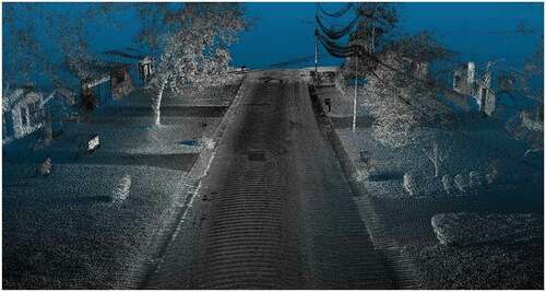
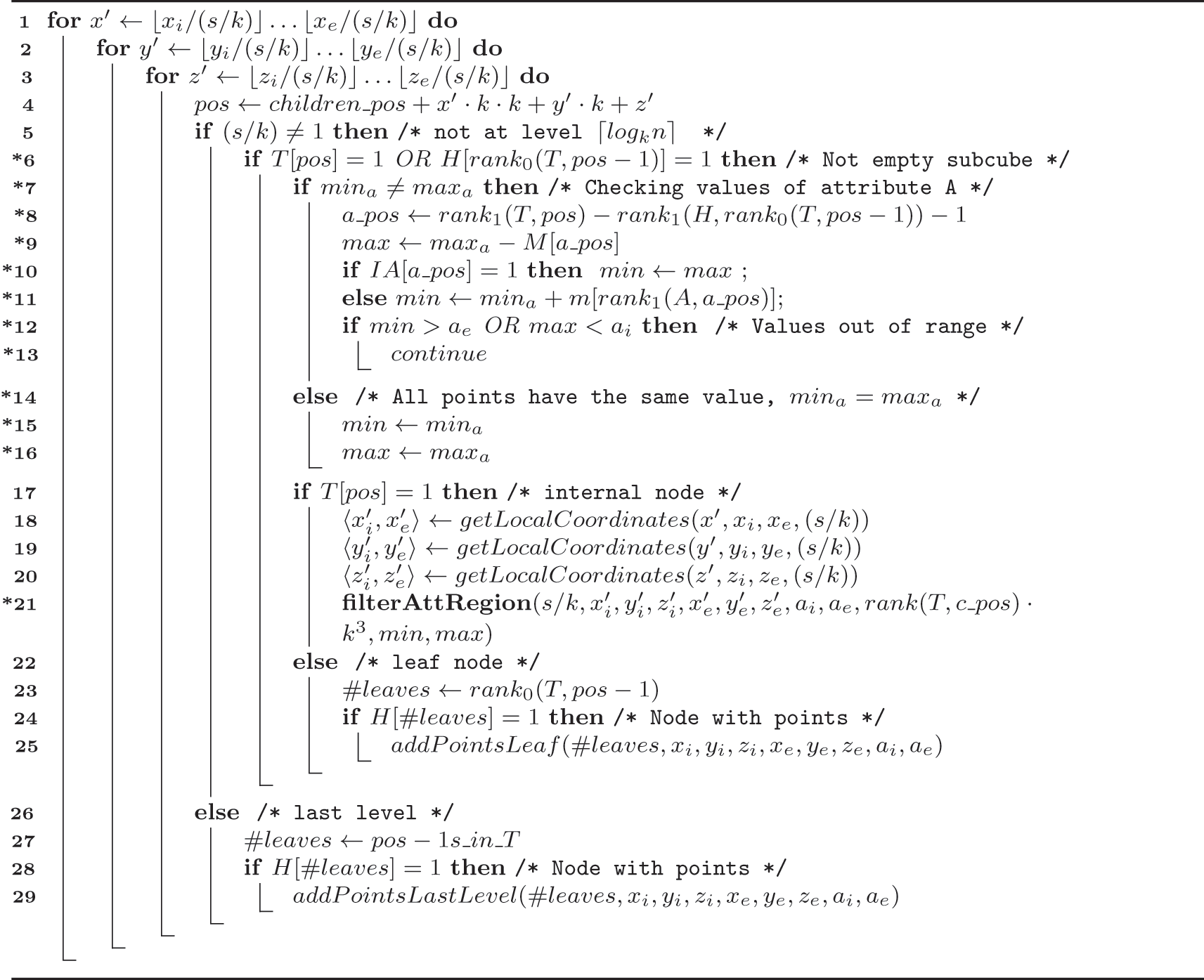
Figure 11. Visualization of the dataset labeled as PNOA-L using the software CloudCompare. The dataset is a point cloud acquired using an aircraft-mounted scanner with a density of at least 0.5 points/m². the dataset is centered on the city of a Coruña (Spain) and it includes a high-density urban area, low-density intermediate areas, and sea areas.

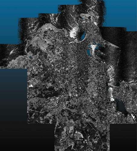
• ISPRS: We used two datasets extracted from the ISPRS benchmark on indoor modeling (Khoshelham et al. 2017).⁶ These datasets are labeled as TUB1 and FireBr. TUB1 is a point cloud captured in one of the buildings of the Technische Universitat Braunschweig, Germany, while FireBr represents an office of the fire brigade in Delft, the Netherlands. These datasets only contain the point coordinates, being the rest of the additional attributes empty.

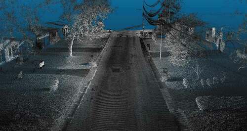
• LidarUSA: We used five datasets from LidarUSA sample data.⁷ The first three datasets (Velo1, Velo2, and Velo3) correspond to data collected from the back of a truck using a Velodyne HD32 scanner in a busy urban environment. The other two datasets (Ladyb1 and Ladyb2) correspond to data with a Scanlook Snoopy A-Series mounted on a truck and then colorized along with the corresponding Ladybug5 imagery. Figures 12 and 13 show a general and detailed visualization of dataset Ladyb2.

Figure 12. Visualization of the dataset labeled as Ladyb2 using the software CloudCompare. The dataset is a point cloud acquired using a truck-mounted scanner in a residential area and it includes a street, some trees and house facades.

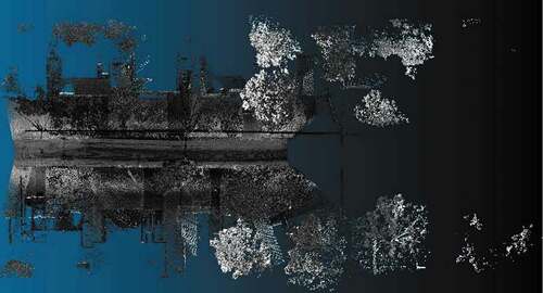
Figure 13. Detail of the Ladyb2 described in Figure 12.

Table 1 and Table 2 show the main properties of the datasets. For each one, we include the number of points, the maximum and minimum value for each coordinate, both the original value and also the converted one, which is used in the representation, and the range of values of the attributes it contains (intensity, return number, number of returns, edge of flight line, scan direction flag, classification, scan angle rank, and point source id). Datasets TUB1 and FireBr do not include any attribute, and datasets from LiDarUSA source only include intensity, scan angle rank, and point source id attributes.

Table 1. Dataset description. We show the number of points, the minimum and maximum values for the real coordinates $x,y,z$, and the maximum $x,y,z$ values, after the coordinates are converted (scaled and translated using an offset).

	PNOA-S	PNOA-M	PNOA-L	TUB1	FireBr
#points	13,265,144	25,108,130	52,627,503	32,597,694	10,406,389
min x (real)	546,000.00	544,000.00	542,000.00	−9.90	44.32
max x (real)	549,999.99	549,999.99	551,999.99	5.76	58.40
min y (real)	4,798,000.00	4,798,000.00	4,794,000.00	−24.52	23.10
max y (real)	4,801,999.99	4,803,999.99	4,805,020.45	18.30	77.67
min z (real)	−39.14	−162.43	−162.43	−1.46	1.27
max z (real)	179.58	1005.05	1005.05	1.10	12.04
max X (conv.)	3,999,990	5,999,990	9,999,990	${10}^9$	${10}^9$
max Y (conv.)	3,999,990	5,999,990	11,020,450	${10}^9$	${10}^9$
max Z (conv.)	218,720	1,167,480	1,167,480	${10}^9$	${10}^9$
intensity	[0, 255]	[0, 255]	[0, 255]
return number	[1,4]	[1,4]	[1,4]
#returns	[1,4]	[1,4]	[1,4]
edge flight line	[0,1]	[0,1]	[0,1]
scan direction	[0,1]	[0,1]	[0,1]
classification	[1,7]	[1,7]	[1,7]
scan angle	[−24,25]	[−24,25]	[−25,28]
point source	[176,244]	[176,226]	[175,227]

Table 2. Dataset description. We show the number of points, the minimum and maximum values for the real coordinates $x,y,z$, and the maximum $x,y,z$ values, after the coordinates are converted (scaled and translated using an offset).

	Velo1	Velo2	Velo3	Ladyb1	Ladyb2
#points	10,000,414	10,002,027	10,001,404	10,001,535	4,295,200
min x (real)	623,346.98	623,131.56	622,919.91	2,241,515.76	2,242,107.25
max x (real)	623,663.73	623,481.06	623,245.05	2,242,377.00	2,242,614.25
min y (real)	698,246.92	698,287.45	698,340.70	1,742,298.86	1,742,299.38
max y (real)	698,486.03	698,532.89	698,574.82	1,742,556.94	1,742,554.63
min z (real)	7.76	8.19	13.77	699.89	699.90
max z (real)	104.24	90.11	91.00	791.74	788.87
max X(conv.)	316,754	349,502	325,145	861,243	507,000
max Y (conv.)	239,109	245,444	234,115	258,073	255,250
max Z (conv.)	96,484	81,925	77,234	91,854	88,974
intensity	[0, 255]	[0, 255]	[0, 255]	[0, 255]	[0, 255]
scan angle	[−90,90]	[−90,90]	[−90,90]	[−90,90]	[−90,90]
point source	[0,31]	[0,31]	[0,31]	[0,31]	[0,31]

We include in Appendix A the visualization of all the datasets. Figures 11, 12 and 13 show the visualization of the largest and smallest datasets, i.e. PNOA-L and Ladyb2. We have used the open-source software CloudCompare⁸ to create the visualizations displaying the point intensity using a grayscale. For ISPRS datasets (i.e. TUB1 and FireBr), we have also included a visualization using an eye-dome lighting (EDL) shader. EDL is a non-photorealistic, image-based shading technique designed to improve depth perception in scientific visualization images (Ribes and Boucheny 2017).

5.3. Query sets and benchmarking setup

We report average CPU time needed by each method for running a set of random queries. The sets of queries are randomly created beforehand for each type of query, such that all techniques run the same sets of queries. The queries are executed in batch mode on the compressed point cloud, running the queries consecutively, starting the next query as soon as the previous one ends. In the case of LAZ, the LAX file is also created beforehand, and is not rebuilt when executing the queries, just loaded before the query set is launched. In the case of ${\mathrm{k}}^3-\mathrm{l}\mathrm{i}\mathrm{d}\mathrm{a}\mathrm{r}$ and ${\mathrm{k}}_{\mathrm{i}}^3-\mathrm{l}\mathrm{i}\mathrm{d}\mathrm{a}\mathrm{r}$, the compact data structure is also created beforehand, and the complete data structure is loaded into the main memory before running the query set.

Table 3 shows, for each type of query and for each dataset, the number of queries included in each query set and the number of points recovered after running those queries. In the case of the query getRegion, the queries consist of a 3D region defined by two 3D points. In the case of the query getRegionXY, the queries consist of a 2D region defined by two 2D points. In the case of the query filterAttRegion, the queries consist of a 3D region defined by two 3D points and a range of two values. For each query, the coordinate values of the points and the range values are chosen randomly between the minimum and maximum of the possible values, such that they are valid regions of the point cloud and valid ranges for the indexed attribute.

Table 3. Query set description. We show the number of random queries generated for each dataset and type of query, and the number of points recovered by each query set.

	getRegion		getRegionXY		filterAttRegion
	#	# recov.	#	# recov.	#	# recov.
Dataset	queries	points	queries	points	queries	points
PNOA-S	385	403,101,444	427	928,104,816	383	137,136,273
PNOA-M	255	726,373,357	466	2,114,689,801	193	200,265,173
PNOA-L	304	1,775,203,414	446	5,558,524,972	214	472,055,725
TUB1	427	1,004,335,863	431	3,529,701,353
FireBr	416	231,777,820	428	665,774,913
Velo1	426	320,454,223	473	1,626,998,431	334	88,292,206
Velo2	415	389,749,715	439	1,300,906,010	406	125,592,346
Velo3	425	280,165,398	456	1,222,284,837	388	62,673,909
Ladyb1	385	190,312,415	424	1,164,475,358	362	52,378,075
Ladyb2	405	88,517,554	454	553,178,511	368	18,673,499

5.4. Space requirements

The comparison of space is shown in Table 4. We report the space required by each method when representing the datasets with all their attributes. We include two alternatives for ${\mathrm{k}}^3-\mathrm{l}\mathrm{i}\mathrm{d}\mathrm{a}\mathrm{r}$ and ${\mathrm{k}}_{\mathrm{i}}^3-\mathrm{l}\mathrm{i}\mathrm{d}\mathrm{a}\mathrm{r}$ depending on how the coordinates are being represented: using three arrays (column $X,Y,Z$) or just one array (column $P$). In the case of LAZ, the reported space also includes the size of LAX file. The size of this file is negligible in comparison to the size of the datasets (for these datasets, around 15–110 KB).

Table 4. Comparison of the space (MB) for the different approaches over all datasets. We include two alternatives for ${\mathrm{k}}^3-\mathrm{l}\mathrm{i}\mathrm{d}\mathrm{a}\mathrm{r}$ and ${\mathrm{k}}_{\mathrm{i}}^3-\mathrm{l}\mathrm{i}\mathrm{d}\mathrm{a}\mathrm{r}$ depending on how the coordinates are being represented: using three arrays (column $X,Y,Z$) or just one array (column $P$) The best value is in bold.

		Space (MB)
				${\mathrm{k}}^3-\mathrm{l}\mathrm{i}\mathrm{d}\mathrm{a}\mathrm{r}$		${\mathrm{k}}_{\mathrm{i}}^3-\mathrm{l}\mathrm{i}\mathrm{d}\mathrm{a}\mathrm{r}$
Dataset	# points	LAS	LAZ	$X,Y,Z$	$P$	$X,Y,Z$	$P$
PNOA-S	13,265,144	254.0	42.4	112.6	109.3	114.5	111.2
PNOA-M	25,108,130	479.0	79.7	213.8	207.6	217.5	211.3
PNOA-L	52,627,503	1004.0	172.8	448.8	435.8	456.7	443.6
TUB1	32,597,694	622.0	195.2	288.5	287.6	291.6	291.0
FireBr	10,406,389	199.0	76.9	97.4	97.4	99.0	99.0
Velo1	10,001,496	191.0	58.2	62.4	59.6	63.7	60.9
Velo2	10,002,229	191.0	60.0	64.7	61.9	66.0	63.3
Velo3	10,002,080	191.0	59.5	64.7	61.9	66.0	63.3
Ladyb1	10,001,543	191.0	59.7	67.0	64.5	68.5	65.9
Ladyb2	4,447,430	85.0	22.5	23.8	22.1	24.4	22.8

LAZ files obtain the best results in almost all cases, especially for the first five datasets extracted from PNOA and ISPRS data sources. However, our techniques achieve almost the same compact space as LAZ for the datasets extracted from LidarUSA. In particular, for Ladyb2, our version using just one array for representing the coordinate values outperforms LAZ in terms of space requirements. This good behavior of our approach for LidarUSA datasets is due to the fact that LidarUSA clouds are very dense, and they can be compactly captured by our proposal. However, both PNOA and ISPRS are much sparse 3D point clouds, which require a higher number of levels of the tree and higher numbers for representing the coordinates, which worsens the compression rate of their DACs representation.

Compared with the uncompressed format, LAZ shows a compression rate that ranges between 16.6% and 38.6% of the space required by LAS format. Our approaches obtain spaces lower than half the space required by LAS for all datasets (ranging 26.0%–48.7% of LAS format). We can also see that our approach ${\mathrm{k}}_{\mathrm{i}}^3-\mathrm{l}\mathrm{i}\mathrm{d}\mathrm{a}\mathrm{r}$ requires around 1%–3% more space than ${\mathrm{k}}^3-\mathrm{l}\mathrm{i}\mathrm{d}\mathrm{a}\mathrm{r}$. This is due to the attribute indexes, which require a bit of extra space, but will allow more efficient filterAttRegion queries, as we will see in the next sections.

Table 5 shows the comparison of space used in main memory running a query, specifically getRegion. LAZ obtains the best results in all cases and, furthermore, does not show variation for datasets of different nature. LAZ is stored on disk during the execution of the query. Thus, it is not necessary to load the whole file into the main memory.

Table 5. Comparison of the peak of space (MB) consumption running the query getRegion for the different approaches over all datasets. We include two alternatives for ${\mathrm{k}}^3-\mathrm{l}\mathrm{i}\mathrm{d}\mathrm{a}\mathrm{r}$ and ${\mathrm{k}}_{\mathrm{i}}^3-\mathrm{l}\mathrm{i}\mathrm{d}\mathrm{a}\mathrm{r}$ depending on how the coordinates are being represented: using three arrays (column $X,Y,Z$) or just one array (column $P$).

	Space (MB)
		${\mathrm{k}}^3-\mathrm{l}\mathrm{i}\mathrm{d}\mathrm{a}\mathrm{r}$		${\mathrm{k}}_{\mathrm{i}}^3-\mathrm{l}\mathrm{i}\mathrm{d}\mathrm{a}\mathrm{r}$
Dataset	LAZ	$X,Y,Z$	$P$	$X,Y,Z$	$P$
PNOA-S	17	128	125	130	127
PNOA-M	18	230	224	234	227
PNOA-L	16	465	452	473	460
TUB1	16	305	304	308	307
FireBr	16	113	113	115	115
Velo1	17	78	75	80	77
Velo2	17	81	78	82	79
Velo3	17	81	78	82	79
Ladyb1	17	83	80	84	82
Ladyb2	17	40	38	40	39

Comparing the results with the values in Table 4, we observe that the memory consumption is proportional to the space used to represent our structure. Recall that our solution is designed to reside in main memory all the time. Therefore, most of the consumption is due to the structure itself and our algorithm does not require much additional memory. In this case, the ${\mathrm{k}}_{\mathrm{i}}^3-\mathrm{l}\mathrm{i}\mathrm{d}\mathrm{a}\mathrm{r}$ structure has a slightly higher consumption than the ${\mathrm{k}}^3-\mathrm{l}\mathrm{i}\mathrm{d}\mathrm{a}\mathrm{r}$ because it also has to include the indexes on the attributes.

5.5. Construction time

Table 6 shows the comparison among different approaches when measuring the construction time from a LAS file. In this case, we measured real-time, which also includes the disk-access times.

Table 6. Construction time (real time, in seconds) for the different approaches over all datasets. We breakdown the construction time for LAZ to show separately the process of creating the LAZ representation and the LAX file. For ${\mathrm{k}}^3-\mathrm{l}\mathrm{i}\mathrm{d}\mathrm{a}\mathrm{r}$ and ${\mathrm{k}}_{\mathrm{i}}^3-\mathrm{l}\mathrm{i}\mathrm{d}\mathrm{a}\mathrm{r}$ we include two alternatives depending on how the coordinates are being represented: using three arrays (column $X,Y,Z$) or just one array (column $P$) The best value is in bold.

		Time (s)
		LAZ			${\mathrm{k}}^3-\mathrm{l}\mathrm{i}\mathrm{d}\mathrm{a}\mathrm{r}$		${\mathrm{k}}_{\mathrm{i}}^3-\mathrm{l}\mathrm{i}\mathrm{d}\mathrm{a}\mathrm{r}$
Dataset	# points	LAZ	LAX	Total	$X,Y,Z$	$P$	$X,Y,Z$	$P$
PNOA-S	13,265,144	1.85	2.59	4.44	5.16	4.72	5.57	5.07
PNOA-M	25,108,130	3.52	4.98	8.50	10.19	9.32	11.05	9.90
PNOA-L	52,627,503	7.45	10.05	17.50	23.10	19.78	23.12	21.04
TUB1	10,406,389	4.58	5.03	9.61	12.48	16.67	18.71	12.84
FireBr	32,597,694	1.56	1.88	3.44	3.98	3.83	4.53	4.23
Velo1	10,001,496	1.48	2.25	3.73	4.05	3.55	4.35	3.77
Velo2	10,002,229	1.46	2.28	3.74	4.68	3.54	4.19	3.7
Velo3	10,002,080	1.44	2.32	3.76	4.00	3.55	4.23	3.76
Ladyb1	10,001,543	1.49	2.38	3.87	3.80	3.40	4.13	3.69
Ladyb2	4,447,430	0.65	0.94	1.59	1.67	1.50	1.77	1.61

For LAZ files, we break down the time reporting that required just to obtain the LAZ representation and also the building time of the LAX indexes. The construction of LAX indexes accounts for between 52% and 62% of the total construction time. As we can observe in the results, all methods have a comparable construction time. LAZ is faster for PNOA and ISPRS datasets, whereas ${\mathrm{k}}^3-\mathrm{l}\mathrm{i}\mathrm{d}\mathrm{a}\mathrm{r}$ using just one array $P$ for the coordinates is the fastest method for LidarUSA datasets. The construction times obtained by ${\mathrm{k}}^3-\mathrm{l}\mathrm{i}\mathrm{d}\mathrm{a}\mathrm{r}$ are consistent with the space results obtained by this technique. The final data structure is more compact, and it requires less time to be created.

5.6. Query times

Table 7 shows the results for queries getRegion and getRegionXY. We only show here the results obtained by ${\mathrm{k}}^3-\mathrm{l}\mathrm{i}\mathrm{d}\mathrm{a}\mathrm{r}$, as these queries only require accessing the coordinates of the LiDAR points and not the values of the attributes; thus, the indexes over the attributes of ${\mathrm{k}}_{\mathrm{i}}^3-\mathrm{l}\mathrm{i}\mathrm{d}\mathrm{a}\mathrm{r}$ do not present any advantage. We can see that our approach ${\mathrm{k}}^3-\mathrm{l}\mathrm{i}\mathrm{d}\mathrm{a}\mathrm{r}$ clearly outperforms LAZ, being around one order of magnitude faster for all datasets for getRegion query. More concretely, ${\mathrm{k}}^3-\mathrm{l}\mathrm{i}\mathrm{d}\mathrm{a}\mathrm{r}$ is between 8 and 47 times faster than LAZ. In the case of getRegionXY query, ${\mathrm{k}}^3-\mathrm{l}\mathrm{i}\mathrm{d}\mathrm{a}\mathrm{r}$ is between 4 and 7 times faster than LAZ. Among the two approaches for representing the coordinates in our ${\mathrm{k}}^3-\mathrm{l}\mathrm{i}\mathrm{d}\mathrm{a}\mathrm{r}$ technique , the one that uses one array obtains the best performance for getRegion, but without filtering by the Z coordinate (getRegionXY) the version using three arrays achieves better times.

Table 7. Comparison of the time results for getRegion and getRegionxy queries (user CPU time, in microseconds per retrieved point) for the different approaches over all datasets. We include two alternatives for ${\mathrm{k}}^3-\mathrm{l}\mathrm{i}\mathrm{d}\mathrm{a}\mathrm{r}$ and ${\mathrm{k}}_{\mathrm{i}}^3-\mathrm{l}\mathrm{i}\mathrm{d}\mathrm{a}\mathrm{r}$ depending on how the coordinates are being represented: using three arrays (column $X,Y,Z$) or just one array (column $P$) The best value is in bold.

	getRegion ($\mu$s/point)			getRegionXY ($\mu$s/point)
		${\mathrm{k}}^3-\mathrm{l}\mathrm{i}\mathrm{d}\mathrm{a}\mathrm{r}$			${\mathrm{k}}^3-\mathrm{l}\mathrm{i}\mathrm{d}\mathrm{a}\mathrm{r}$
Dataset	LAZ	$X,Y,Z$	$P$	LAZ	$X,Y,Z$	$P$
PNOA-S	0.814	0.077	0.075	0.387	0.073	0.080
PNOA-M	0.594	0.076	0.073	0.339	0.072	0.077
PNOA-L	0.675	0.077	0.071	0.305	0.074	0.079
TUB1	1.709	0.086	0.084	0.611	0.083	0.088
FireBr	1.507	0.074	0.080	0.438	0.072	0.082
Velo1	2.479	0.076	0.068	0.221	0.042	0.046
Velo2	1.678	0.074	0.069	0.551	0.117	0.124
Velo3	2.475	0.076	0.072	1.386	0.335	0.359
Ladyb1	3.068	0.071	0.070	0.349	0.047	0.050
Ladyb2	3.566	0.076	0.076	2.794	0.460	0.522

We can observe that, even than LAZ creates an index for $x$ and $y$ coordinates, we obtain significantly better results when only those coordinates are used in the query, that is, for getRegionXY query. Moreover, as expected, for queries requiring the third dimension, that is, for getRegion queries, ${\mathrm{k}}^3-\mathrm{l}\mathrm{i}\mathrm{d}\mathrm{a}\mathrm{r}$ shows a remarkable superior performance, as LAZ with LAX does not natively support this functionality. Thus, for those datasets requiring similar space, such as those extracted from LidarUSA, ${\mathrm{k}}^3-\mathrm{l}\mathrm{i}\mathrm{d}\mathrm{a}\mathrm{r}$ is the perfect choice when considering the space/time trade-off.

Another interesting property of our approach is that it does not show a high variance in the time results (measured in microseconds per retrieved point); thus, it presents a more stable performance independently of the nature of the input dataset.

Table 8 shows the results for query filterAttRegion when applying a filter over the attribute intensity. We can see here that the ${\mathrm{k}}_{\mathrm{i}}^3-\mathrm{l}\mathrm{i}\mathrm{d}\mathrm{a}\mathrm{r}$ obtains the best results for all cases, in particular, the version using one array for representing the coordinates. It is on average 20% faster than ${\mathrm{k}}^3-\mathrm{l}\mathrm{i}\mathrm{d}\mathrm{a}\mathrm{r}$ and between 11 and 107 times faster than LAZ. Again, our approach shows a more stable performance independently of the nature of the input dataset, which is a desirable property.

Table 8. Comparison of the time results for filterAttregion query (user CPU time, in microseconds per retrieved point) filtering by attribute intensity for the different approaches over all datasets containing that attribute. We include two alternatives for ${\mathrm{k}}^3-\mathrm{l}\mathrm{i}\mathrm{d}\mathrm{a}\mathrm{r}$ and ${\mathrm{k}}_{\mathrm{i}}^3-\mathrm{l}\mathrm{i}\mathrm{d}\mathrm{a}\mathrm{r}$ depending on how the coordinates are being represented: using three arrays (column $X,Y,Z$) or just one array (column $P$) The best value is in bold.

	filterAttRegion ($\mu$s/point)
		${\mathrm{k}}^3-\mathrm{l}\mathrm{i}\mathrm{d}\mathrm{a}\mathrm{r}$		${\mathrm{k}}_{\mathrm{i}}^3-\mathrm{l}\mathrm{i}\mathrm{d}\mathrm{a}\mathrm{r}$
Dataset	LAZ	$X,Y,Z$	$P$	$X,Y,Z$	$P$
PNOA-S	2.449	0.145	0.142	0.132	0.122
PNOA-M	1.468	0.138	0.138	0.129	0.120
PNOA-L	1.669	0.138	0.136	0.126	0.114
Velo1	7.068	0.188	0.176	0.117	0.101
Velo2	5.222	0.141	0.146	0.117	0.109
Velo3	10.230	0.173	0.180	0.138	0.129
Ladyb1	10.588	0.158	0.161	0.129	0.120
Ladyb2	15.404	0.176	0.193	0.160	0.144

5.7. Varying the value of the threshold $l$

In the previous sections, we have used a fixed value of $l=100$ for comparing the results of our method with those obtained by LAS and LAZ. However, this parameter, which determines the stop condition in the building process, may affect both the time performance and the space consumption. In general, when solving getRegion or getRegionXY queries, a higher number of points per leaf node, i.e. setting a high value for $l$, implies shorter trees, and thus better time performance. This is due to the fact that the top-down traversals on the tree needed to obtain the points at the leaves require a lower number of rank operations when the tree is shorter; thus, reducing the overall query time. However, they can require larger memory consumption in the case of ${\mathrm{k}}^3-\mathrm{l}\mathrm{i}\mathrm{d}\mathrm{a}\mathrm{r}$, as the representation is not exploiting the compressibility of those points. On the contrary, the ${\mathrm{k}}_{\mathrm{i}}^3-\mathrm{l}\mathrm{i}\mathrm{d}\mathrm{a}\mathrm{r}$ uses less memory for high values of $l$, as low values of $l$ imply a higher number of levels of the tree, and also require a larger space of the attribute index. It is also interesting the behavior for filterAttRegion queries. In this case, having a high number of points in the leaves requires a longer process of filtering those points by attribute value. Thus, intermediate values for $l$ is a good choice when considering time performance, as small values of $l$ imply trees with a high number of levels, which are neither efficient in terms of time. Of course, this is highly dependent on the dataset and it should be configured for each dataset to obtain the best space/time trade-off.

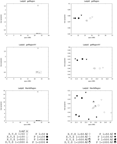
Figures 14 and 15 show the space/time trade-off for different configurations of our approach for the three queries over datasets PNOA-L and Ladyb2. We have chosen those two datasets as they are the largest and smallest in terms of number of points, respectively. In the left part of each figure, we also show the space/time results for LAZ. As LAZ obtains significantly higher time results in all cases, we zoom the part of the figure that includes the results of the variations of our approach. These extracts of the plots are shown in the right part of the figure.

Figure 14. Space/time trade-off for different configurations over PNOA-L dataset when computing the three different types of queries. In the left part, we include the results for LAZ and for the four versions of our method varying threshold $l$. In the right part of the figure, we zoom the figure to better illustrate the differences among the different configurations of our approach. We denote $X,Y,Z$ the version using three different arrays for representing the coordinates and $P$ the one using one unique array. We marked with the text ‘AI’ the configuration including an index over attribute intensity.

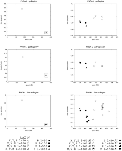
Figure 15. Space/time trade-off for different configurations over Ladyb2 dataset when computing the three different types of queries. In the left part, we include the results for LAZ and for the four versions of our method varying threshold $l$. In the right part of the figure, we zoom the figure to better illustrate the differences among the different configurations of our approach. We denote $X,Y,Z$ the version using three different arrays for representing the coordinates and $P$ the one using one unique array. We marked with the text ‘AI’ the configuration including an index over attribute intensity.

In the case of PNOA-L, we can see the expected behavior. For ${\mathrm{k}}^3-\mathrm{l}\mathrm{i}\mathrm{d}\mathrm{a}\mathrm{r}$, the best space results are obtained with small values of $l$, whereas the best time results are obtained with high values of $l$. On the other hand, for ${\mathrm{k}}_{\mathrm{i}}^3-\mathrm{l}\mathrm{i}\mathrm{d}\mathrm{a}\mathrm{r}$, the best space results are obtained for high values of $l$, whereas the best time performance in the filterAttRegion query is obtained for $l=100$ and using three arrays for representing the coordinates.

In the case of Ladyb2, the best time and space results of ${\mathrm{k}}^3-\mathrm{l}\mathrm{i}\mathrm{d}\mathrm{a}\mathrm{r}$ are obtained with high values of $l$. This differs from the results obtained for the PNOA-L dataset, where the best space results were obtained for a low value of $l$. This is caused by the fact that the points of the Ladyb2 LiDAR cloud are less clustered, more sparse, and thus, having a high number of levels in the tree does not exploit any compressibility of the dataset. For ${\mathrm{k}}_{\mathrm{i}}^3-\mathrm{l}\mathrm{i}\mathrm{d}\mathrm{a}\mathrm{r}$, again, the best time performance in the filterAttRegion query is obtained for $l=100$ and using three arrays for representing the coordinates. It is also worth noting that LAZ is clearly outperformed here both in space and time by several configurations of our approach, namely, ${\mathrm{k}}^3-\mathrm{l}\mathrm{i}\mathrm{d}\mathrm{a}\mathrm{r}$ and ${\mathrm{k}}_{\mathrm{i}}^3-\mathrm{l}\mathrm{i}\mathrm{d}\mathrm{a}\mathrm{r}$ using just one array $P$ for representing the coordinates and using high values for $l$.

5.8. Discussion

Next, we discuss the results of the experiments. The most important contribution of our proposal is that it efficiently supports searches involving the third spatial dimension or the additional attributes, due to the fact that ${\mathrm{k}}^3-\mathrm{l}\mathrm{i}\mathrm{d}\mathrm{a}\mathrm{r}$ has indexes on them, whereas LAZ/LAX does not. This has a direct implication in the time performance of these types of queries.

Moreover, our proposal also outperforms LAZ/LAX for searches that only include constraints on $x$ and $y$ coordinates. This is because our ${\mathrm{k}}^3-\mathrm{l}\mathrm{i}\mathrm{d}\mathrm{a}\mathrm{r}$ is a real random-access compressor, so it only has to recover/decompress the data the user requested, which are stored already at the leaves of our compact octree. Derived from this, two consequences arise. First, to obtain real random access, the compression techniques on which our method is based, basically DACs and delta encoding, are simple, but as a side effect, they are fast. However, the second consequence is that ${\mathrm{k}}^3-\mathrm{l}\mathrm{i}\mathrm{d}\mathrm{a}\mathrm{r}$ compression power is lower, compared to the prediction methods coupled with an arithmetic coder of LAZ.

On the contrary, LAZ is not a real random-access method. To obtain some sort of random access, LAZ divides the data into chunks, with recommended size of 50,000 points, and even when only a small part of a chunk is needed, the complete chunk has to be decompressed. For example, in Figure 1, chunks 1, 2, and 3 must be completely decompressed even when only the shaded regions may have points of interest. Finally, the compression of the coordinates of LAZ is based on a predictor that needs to check the five previous values to make a prediction, and then, the difference between the prediction and the actual value is encoded with an arithmetic encoder. During the decompression, that prediction must be also done and the arithmetic decompression is known to be very slow (Brisaboa et al. 2007).

Moreover, the traditional setup of LAZ/LAX implies two main drawbacks. First, the (spatial) index is an auxiliary structure separated from the data, so when a leaf of the index is reached, a pointer must be followed to access the data file. Second, the pointer points to a disk position, and the access could be slow. Another problem is that, as explained in Section 2.1.2, the pointers at leaves are indeed intervals; moreover, each leaf can have several intervals due to the fact that it is a streaming and order-preserving compressor. Thus, when searching a region, each affected leaf adds a list of intervals. In order to speed up the inspection of these intervals, LAX pays an extra time merging them, trying to get a lower number of less fragmented intervals.

On the other hand, as we already saw, ${\mathrm{k}}^3-\mathrm{l}\mathrm{i}\mathrm{d}\mathrm{a}\mathrm{r}$ consumes more main memory, as it is expected because it uses a compact data structure approach, and thus, it has to keep all the data in main memory all the time, whereas LAZ only loads the disk blocks it needs at each moment, and after using them, they can be deleted from main memory.

6. Conclusions

In this paper, we have presented a new representation for LiDAR point clouds that not only requires very compact spaces, similar to those obtained by state-of-the-art methods such as LAZ but, more importantly, it supports the efficient computation of queries over the compressed data. It solves typical queries, such as obtaining all the points in a 2D or 3D region between 4 and 47 times faster than the state-of-the-art methods. In addition, it offers the possibility to efficiently retrieve the points in a region filtered by an attribute value. Our approach computes these queries 11–88 faster than LAZ. Moreover, we also present a variant of our approach that adds an index over the attributes and, with around 1%–3% of extra space, improves these kinds of queries, being up to 107 faster than LAZ.

Our approach is configurable so it can be adapted to the different nature of the datasets. We include several options, such as different approaches to compact coordinate values or the number of points in the leaf nodes. This allows us to obtain different space/time trade-offs.

As future work, we will extend our technique to support additional queries over LiDAR point clouds and also explore the use of our approach for integrating it into visualization tools for LiDAR point clouds, as our tree-shaped representation can be of interest to efficiently manage the visualization of complex point clouds, in particular zoom-in and zoom-out functionalities.

Another research line would be to turn ${\mathrm{k}}^3-\mathrm{l}\mathrm{i}\mathrm{d}\mathrm{a}\mathrm{r}$ updatable, since it is a static data structure. This is not a big issue for LiDAR data, as acquiring LiDAR data is expensive, thus the updating rate of this type of data is low. Moreover, re-creating the compressed representation from scratch is not a costly process, as shown in our experiments of construction time, compared to the time required by detecting changes on the LiDAR data and updating its compressed representation. However, a dynamic version of our proposal could be of interest in other domains. This dynamic version will be based on practical implementations of dynamic bitmaps that have been presented in recent years (Cordova and Navarro 2016; Prezza 2017).

Disclosure statement

No potential conflict of interest was reported by the author(s).

Data availability statement

The source code of k³ – lidar and k_i³ – lidar is publicly available in the following repository: https://gitlab.lbd.org.es/fsilva/k3-lidar/.

The datasets PNOA-S, PNOA-M, and PNOA-L are a derived work of LIDAR 1st Coverage (2008–2015) CC-BY Organismo Autónomo Centro Nacional de Información Geográfica (CNIG). CNIG grants permissions to use the datasets and to generate derived datasets for any purpose as long as the creator is attributed. Our derived datasets are openly available in figshare at https://figshare.com/collections/LiDAR/5720168, reference number 5,720,168.

The datasets TUB1 and FireBr are part of the ISPRS Benchmark on Indoor Modeling (Khoshelham et al. 2017) and can be downloaded from https://www2.isprs.org/commissions/comm4/wg5/benchmark-on-indoor-modelling. ISPRS grants permission to use the datasets for research purposes only, and it does not allow the datasets to be distributed. They have to be downloaded from the ISPRS website using the link above.

The datasets Velo1, Velo2, Velo3, Ladyb1, and Ladyb2 are available on request from the website of LidarUSA at https://www.lidarusa.com/sample-data.html. We have contacted a representative from the company that has granted us usage of the datasets for research purposes.

The query sets used in the experimental evaluation to measure time performance are openly available in figshare at https://figshare.com/collections/LiDAR_Queries/5915297, reference number 5,915,297.

Additional information

Funding

This work was supported by CITIC, as Research Center accredited by Galician University System, is funded by “Consellera de Cultura, Educación e Universidade from Xunta de Galicia”, supported in an 80% through ERDF Funds, ERDF Operational Programme Galicia 2014–2020, and the remaining 20% by “Secretara Xeral de Universidades” (Grant ED431G 2019/01), Xunta de Galicia/FEDER-UE under Grants [ED431C 2021/53; IG240.2020.1.185]; Ministerio de Ciencia e Innovación under Grants [PID2020-114635RB-I00; PDC2021-120917-C21; PDC2021-121239-C31; PID2019-105221RB-C41].

Notes on contributors

Susana Ladra

Susana Ladra is Associate Professor at the University of A Coruña, Spain. Her research interests include design and analysis of algorithms and data structures, and data compression and data mining in the fields of information retrieval and bioinformatics.

Miguel R. Luaces

Miguel Rodríguez Luaces received his Ph.D. in Computer Science from the University of A Coruña (Spain) in 2004. He undertook research in the area of spatial, temporal and spatio-temporal databases at the FernUniversität Hagen (Germany) under the ChoroChronos project funded by the European Union. Today, he is an Associate Professor at the University of A Coruña and his research interests include Geographic Information Systems, Spatial and Spatio-temporal Databases, Software Engineering, and Web-based Information Systems.

José R. Paramá

José R. Paramá is Associate Professor at the University of A Coruña, Spain. His research interests include compression and indexation of information, spatial databases, and bioinformatics.

Fernando Silva-Coira

Fernando Silva-Coira received the PhD degree in Computer Science from the University of A Coruña. He is an adjunct at the University of A Coruña. His research interests are compact data structures, algorithms, and spatial databases.

Notes

1. https://www.apple.com/ipad-pro/.

2. In the case of a cube with different sizes in each dimension, we conceptually fill the input data with empty space. This does not significantly affect the final result because our data structure is very efficient at representing the empty areas.

3. Notice that the cube can be defined from two 3D points by just taking a mixture of their elements to get the eight corner vertices in the 3D space.

4. https://github.com/LAStools/LAStoolshttps://github.com/LAStools/LAStools.

5. https://pnoa.ign.es/el-proyecto-pnoa-lidarhttps://pnoa.ign.es/el-proyecto-pnoa-lidar.

6. https://www2.isprs.org/commissions/comm4/wg5/benchmark-on-indoor-modelling/https://www2.isprs.org/commissions/comm4/wg5/benchmark-on-indoor-modelling/.

7. https://www.lidarusa.com/sample-data.htmlhttps://www.lidarusa.com/sample-data.html.

8. https://www.danielgm.net/cc/https://www.danielgm.net/cc/.

Appendix A:

Visualization of the Datasets

Figure A1. Visualization of the dataset labeled as PNOA-S.

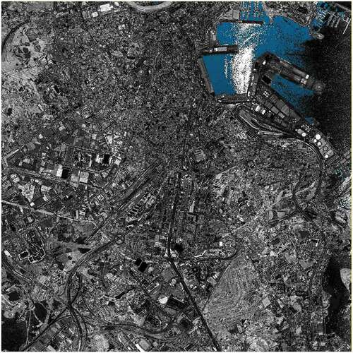
Figure A2. Visualization of the dataset labeled as PNOA-M.

Figure A3. Visualization of the dataset labeled as PNOA-L.

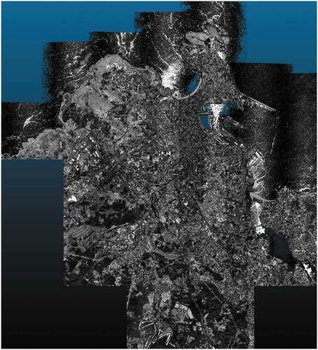
Figure A4. Visualization of the dataset labeled as TUB1.

Figure A5. Visualization of a detail of the dataset labeled as TUB1.

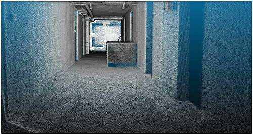
Figure A6. Visualization of a detail of the dataset labeled as TUB1-Detail using an EDL shader.

Figure A7. Visualization of the dataset labeled as FireBr.

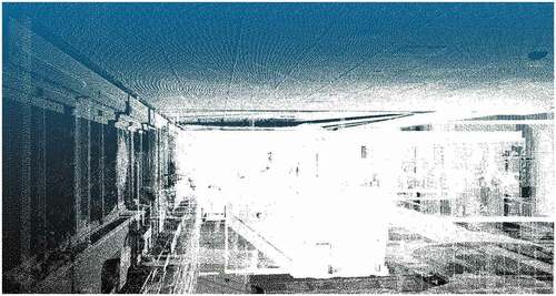
Figure A8. Visualization of a detail of the dataset labeled as FireBr.

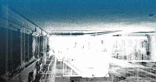
Figure A9. Visualization of a detail of the dataset labeled as FireBr using an EDL shader.

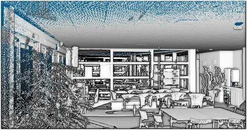
Figure A10. Visualization of the dataset labeled as Velo1.

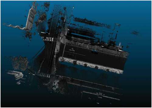
Figure A11. Visualization of a detail of the dataset labeled as Velo1.

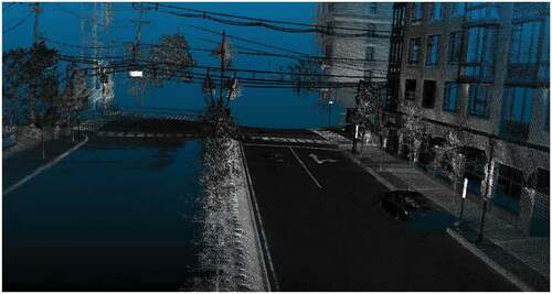
Figure A12. Visualization of the dataset labeled as Velo2.

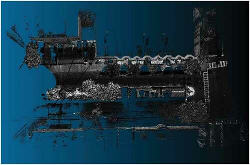
Figure A13. Visualization of a detail of the dataset labeled as Velo2.

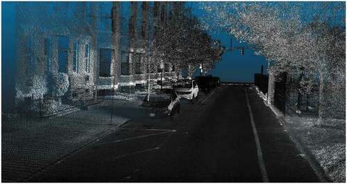
Figure A14. Visualization of the dataset labeled as Velo3.

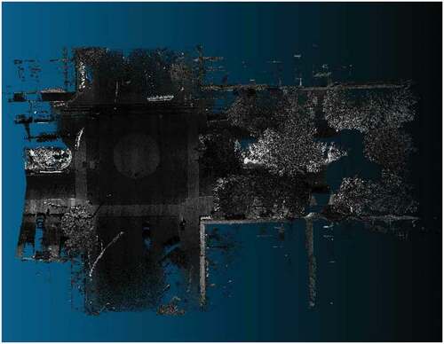
Figure A15. Visualization of a detail of the dataset labeled as Velo3.

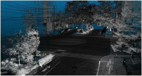
Figure A16. Visualization of the dataset labeled as Ladyb1.

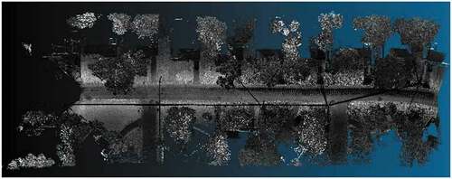
Figure A17. Visualization of a detail of the dataset labeled as Ladyb1.

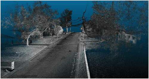
Figure A18. Visualization of the dataset labeled as Ladyb2.

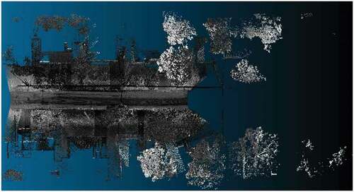
Figure A19. Visualization of a detail of the dataset labeled as Ladyb2.

References

- Abel, D. J., and J. L. Smith. 1983. “A Data Structure and Algorithm Based on a Linear Key for a Rectangle Retrieval Problem.” Computer Vision, Graphics, and Image Processing 24 (1): 1–13. doi:10.1016/0734-189X(83)90017-8.