Unravel the spatio-temporal patterns and their nonlinear relationship with correlates of dockless shared bikes near metro stations

ABSTRACT

The dockless bike-sharing system has rapidly expanded worldwide and has been widely used as an intermodal transport to connect with public transportation. However, higher flexibility may cause an imbalance between supply and demand during daily operation, especially around the metro stations. A stable and efficient rebalancing model requires spatio-temporal usage patterns as fundamental inputs. Therefore, understanding the spatio-temporal patterns and correlates is important for optimizing and rescheduling bike-sharing systems. This study proposed a dynamic time warping distance-based two-dimensional clustering method to quantify spatio-temporal patterns of dockless shared bikes in Wuhan and further applied the multiclass explainable boosting machine to explore the main related factors of these patterns. The results found six patterns on weekdays and four patterns on weekends. Three patterns show the imbalance of arrival and departure flow in the morning and evening peak hours, while these phenomena become less intensive on weekends. Road density, living service facility density and residential density are the top influencing factors on both weekdays and weekends, which means that the comprehensive impact of built-up environment attraction, facility suitability and riding demand leads to the different usage patterns. The nonlinear influence universally exists, and the probability of a certain pattern varies in different value ranges of variables. When the densities of living facilities and roads are moderate and the relationship between job and housing is relatively balanced, it can effectively promote the balanced usage of dockless shared bikes while maintaining high riding flow. The spatio-temporal patterns can identify the associated problems such as imbalance or lack of users, which could be mitigated by corresponding solutions. The relative importance and nonlinear effects help planners prioritize strategies and identify effective ranges on different patterns to promote the usage and efficiency of the bike-sharing system.

KEYWORDS:

• Dockless shared bikes
• spatio-temporal patterns
• machine learning
• transit oriented development

1. Introduction

In the context of global low-carbon economy, environmentally sustainable development and physical health initiatives, shared bikes are widely promoted. Under the rapid rise of the sharing economy, the bike-sharing system has become popular all over the world, especially dockless bike-sharing programs (Liu, Szeto, and Ho 2018). Over 300 cities in China deployed shared bikes by 2019, and the number is further expanding. Although some recent studies critically questioned their contribution to reducing environmental pollution because of management chaos and expensive maintenance costs, in the long run, if management efficiency is improved, the benefit of shared bikes for reducing carbon emissions would be significant (Médard De Chardon 2019; Ricci 2015). In particular, as a feeder mode, shared bikes make metro stations more attractive beyond walking distance (Lin et al. 2019). To achieve the goal of high urban density, sustainable development, and pedestrian- and cycle-friendly urban environments, the concept of Transit Oriented Development (TOD) has been widely accepted (Ibraeva et al. 2020; Shao et al. 2020). The basic philosophy of TOD is channeling mega-city growth in full use of public transit systems, enhancing the sustainability, accessibility, and efficiency of public transportation (Hickman and Hall 2008). The popularity of shared bikes provides a flexible option to improve the efficiency of public transit systems, and their integration has attracted the attention of substantial scholars (Lu et al. 2018; Capodici, D’Orso, and Migliore 2021; Dadhich and Hanaoka 2012). Using bikes to access/depart transit stations is regarded as a time-saving method to solve the first/last mile problem (Lin et al. 2019).

Dockless shared bikes can be stopped anywhere, except for areas prohibited from parking, which saves the space and capital of constructing dock stations (Zhang and Mi 2018). Meanwhile, the flexibility of selecting the origin and destination makes it an important approach to study the user’s travel behavior. However, some problems also follow, such as supply and demand mismatch, low utilization efficiency, and indiscriminate parking (Zhang, Lin, and Mi 2019). For example, a “tidal flow” moves from or to certain regions during morning and evening commuting peaks, leading to some regions being entirely full while others lack shared bikes (Fishman 2015). This phenomenon may hinder the rational distribution of shared bikes, reduce satisfaction, and even aggravate traffic problems (Tan et al. 2021). According to the survey, integration with public transportation is the most common use of dockless shared bikes, which makes the imbalance between supply and demand more serious around the metro station (Li et al. 2021). As the “capillaries” for the transit aorta, the bike trips around transportation hubs help solve the first/last mile problem and facilitate the implementation of the TOD policy (Lin et al. 2019). Therefore, understanding the spatio-temporal usage patterns of shared bikes around metro stations and identifying related factors are necessary to implement effective intervention and management strategies.

Many studies have investigated bike-sharing systems, explored the features and causes of their usage patterns, and proposed rebalancing and optimization strategies (Kou and Cai 2019; Xing, Wang, and Lu 2020; Ji et al. 2020). However, some critical questions have not been well addressed. First, most studies only focus on the intensity of riding flow, or the balance of arrival and departure flow. Few studies completely combine riding intensity and the balance of arrival/departure for pattern division. The imbalance of arrivals and departures in high riding flow areas is often more likely to lead to an imbalance between the supply and demand of shared bikes. For clustering algorithms, Euclidean distance is generally used to measure the difference. Since peaks and troughs of bike-sharing usage are not strictly one-to-one corresponding in the time dimension, the offsets are difficult to be captured by Euclidean distance (Li, Zhao, and Li 2019). Furthermore, previous studies assumed that the effects of variables are linear and ignored the potential thresholds. While the probability of a certain pattern may be the greatest in a specific value range, changing the condition may be infertile in influencing usage patterns once the threshold is reached.

To fill these gaps, this study conducted empirical research on bike-sharing data obtained from Mobike, the world’s largest dockless bike-sharing platform, to explore the spatio-temporal patterns and nonlinear effects of possible variables. This research makes three main contributions. First, bivariate time series clustering was used on two characteristics, total flow (intensity of riding flow) and net flow (balance of arrival and departure flow), and analyzed these two-dimensional patterns, which can better describe the convergence and divergence of shared bikes around metro stations and identify areas prone to “tidal phenomena”. Dynamic Time Warping (DTW) distance was introduced to better capture the similarity among different time series and obtain more effective clustering results. Second, using interpretable machine learning models, the nonlinear and threshold effects of factors on usage patterns were illustrated, thereby providing effective ranges for the implementation of intervention and optimization strategies. For example, high road density may promote cycling, but will this effect continue linearly? This study offers concrete evidence for the thresholds of variables and guides operators and planners to which areas should be given more attention. Third, the different usage patterns and the key variables on weekdays and weekends were compared, further discussing the possible causes. Spatio-temporal patterns can increase the understanding of the usage of shared bikes at the TOD level and identify the associated problems, such as tidal phenomena and lack of users, which could be alleviated by corresponding solutions. Furthermore, the relative importance and nonlinear effects of individual factors can inform policy-makers to prioritize strategies and propose more targeted measures to guide the efficient use of shared bikes, alleviating the first/last mile problem.

This paper is organized as follows: Section 2 introduces the related literature. Section 2 proposes the data and methods to perform the analysis. Section 3 presents the analysis and results. Section 4 provides the discussion and policy implications. Section 5 concludes the study.

2. Literature review

In this section, related research on the usage patterns of shared bikes and their explanatory factors is reviewed. The existing bike-sharing schemes can be divided into two categories: with bike stations (docked bike-sharing schemes) and without bike stations (dockless bike-sharing schemes). Most of the earlier studies were about docked shared bikes, including utilization rate, location optimization of bike-sharing stations, user characteristics, rebalancing measures, temporal usage patterns, and so on (Ma et al. 2020; O’Neill and Caulfield 2012; García-Palomares, Gutiérrez, and Latorre 2012). For instance, Shaheen, Cohen, and Martin (2013) found that gender and income could affect the choice of docked shared bikes; specifically, men and people with higher incomes are more likely to choose docked shared bikes. Kaltenbrunner et al. (2010) performed a case study in Barcelona and found that the utilization rate of docked shared bikes was higher on weekdays than on weekends, and there was a peak in the morning and evening, which means that the main purpose of using docked shared bikes on weekdays may be commuting. Jiménez et al. (2016) classified the bike-sharing stations with three ratios: available bikes ratio, turnover ratio, and cumulative trips ratio. The results showed the spatial imbalance of bike-sharing distribution and confirmed which stations need to avoid low use. Vogel, Greiser, and Mattfeld (2011) used the expectation-maximization algorithm to conduct a cluster analysis of ride flow, revealing different spatio-temporal patterns of pickup and return activities at bike stations. Froehlich, Neumann, and Oliver (2008) investigated the temporal patterns of different bike-sharing stations to reflect human mobility and city dynamics and revealed that the movement patterns were significantly affected by urban layout. Although these results help understand the related factors influencing the demands and usage patterns of shared bikes, the accessibility and flexibility of the docked bike-sharing system are restricted by the location of stations, which hinders its deployment, especially in condensed metropolises with limited available space (Yu, Liu, and Yin 2021). Besides, connectivity of public transit has been identified as one of the main challenges in urban development, and bikes as a connection tool is a feasible and economical way to expand the scope of transit services, which means a more flexible bike-sharing system is needed (Lu et al. 2018).

With the recent emergence of the dockless bike-sharing system and GPS tracking techniques, it provides great convenience for connecting to metro stations and solving the first/last mile problem (Huang and Wang 2020; Shen et al. 2020). Compared to docked shared bikes, the dockless bike-sharing system has two main advantages: (1) It saves the cost and space for constructing the bike-sharing stations and infrastructures. (2) The shared bikes can be rented and returned almost anywhere. Locators are equipped inside dockless shared bikes to record the digital footprints of users, which makes it possible to explore the spatio-temporal usage patterns of shared bikes by having massive amounts of data. The number of studies on dockless bike-sharing systems is limited because these systems have existed for a short time up to now and the data is confidential due to privacy issues. Existing studies found that users of dockless shared bikes were mostly male, younger, company employees and more educated (Li et al. 2018; Xin et al. 2018). Some studies focus on different travel activities of dockless bike users, such as commuting, entertainment, and schooling, which contribute to understanding the main purpose of dockless bike-sharing usage. (Buck et al. 2013; Yang et al. 2019). According to the questionnaire and research results, integration with public transportation is the major purpose of using shared bikes. Sixty-three percent of bike-sharing orders are to connect transportation hubs in Guangzhou, China (Wang et al. 2016). Shen, Zhang, and Zhao (2018) found that the peak value of morning and evening rush time on weekdays was more obvious, whereas the demand trend was smoother on weekends, indicating the fact that trips for commuting purposes dominate on weekdays while more trips for leisure activities take place on weekends. A study on inferring the use purpose of shared bikes based on the gravity model and Bayesian rules found that transfer activities account for the largest proportion of bike-sharing travel, especially around metro hubs, which proved that dockless shared bikes play an important role in the first/last mile connection with metro stations (Li et al. 2021). Furthermore, TOD has been widely advocated, and the study of TOD typology has attracted the attention of researchers (Lyu, Bertolini, and Pfeffer 2016). By analyzing the land use and other indicators around the metro stations, the metro station is divided into different types through clustering methods, and the context-specific typology can guide planners in considering future interventions (Kamruzzaman et al. 2014). Bearing such a trend in mind, the spatio-temporal patterns of dockless shared bikes around metro stations and their characteristics need to be explored, which could guide the improvement of multi-mode transportation systems and promote commuting efficiency.

To date, some research has investigated the spatio-temporal patterns of bike-sharing usage and the connection with transportation hubs. Yang et al. (2019) used graph-based approaches to quantify the influence of metro services on bike-sharing patterns and riding flows, exploring the support of shared bikes over the “last mile.” Li et al. (2020) employed a nondata adaptive representation method to reduce the random error of time series and used k-means to differentiate bike usage patterns. Xing, Wang, and Lu (2020) applied k-means ++ to investigate the demand patterns and trip purpose of dockless shared bikes. Although these studies provide insights into understanding the usage patterns of shared bikes, most were concentrated on a single dimension of riding intensity or the balance of arrival and departure of riding flow. Some studies have introduced the process of convergence and divergence into pattern analysis and conducted empirical research on human mobility to describe the balance of daily activities (Yang et al. 2016; Fang et al. 2017), which the definitions and methods could be transferred to the research on the tidal phenomenon of dockless shared bikes. Besides, the ratios focus on bike stations can also be applied to the dockless bike-sharing schemes (Jiménez et al. 2016). Considering both the intensity and balance of riding flow when analyzing the spatio-temporal pattern of bike-sharing usage can recognize the regions with high riding intensity that remain the balance of arrival/departure and find the regions with large fluctuations over time. Focus was placed on tidal phenomena in regions with more bike-sharing users rather than areas with less riding flow in this study. The bivariate clustering method can better distinguish these regions. Analyzing the two attributes of riding flow can be a more comprehensive perspective for optimizing and rescheduling bike-sharing systems. When performing the cluster analysis of time series data, DTW distance can effectively recognize differences and construct the similarity matrix (Liu et al. 2020; Li, Zhao, and Li 2019; Chabchoub and Fricker 2015), which has great potential in distinguishing the usage patterns of shared bikes.

Additionally, existing studies are mainly based on binary or multiple logistic models to reveal the main causes of usage patterns, which may ignore the potential nonlinear effects of factors and understate the influences of variables within the effective range (Liu, Wang, and Xiao 2021; Chen and Ye 2021). Researchers have recently applied machine learning methods to examine nonlinear relationships in the field of geography and transportation and have proven their effectiveness. Willing et al. (2017) used a Gradient Boosting Machine (GBM) to rank the variables according to their respective influence on carsharing activity. For identifying factors influencing bike-sharing demand, Duran-Rodas, Chaniotakis, and Antoniou (2019) compared three methods and found that GBM was the most suitable regression method to fit the data, followed by generalized linear models. Comprehensively compared with logit models, researchers have found that machine learning outperforms at both the individual and aggregate levels, which has successfully shaken the linear assumption and provided additional nuanced references (Ding, Cao, and Wang 2018). However, current studies have focused on the factors affecting the demand for shared bikes, which is a regression problem, while few studies have investigated factors affecting different usage patterns of shared bikes, which is a multiclass situation. Additionally, each factor may have nonlinear relationships with different usage patterns. If true, the “one size fits all” assumption may provide incorrect estimates of the associations between factors and usage patterns within certain ranges, which hence will mislead planners. Therefore, introducing the interpretable machine learning method to capture the nonlinear and threshold effects of variables on the usage patterns of shared bikes is a meaningful attempt.

3. Methodology

3.1. Study area and data

Wuhan, the core city in central China, has a large population of over 11 million and a total area of 8569 km² in 2019. The urban center is situated at the intersection where the Yangtze and Han Rivers meet (Figure 1). With the rapid increase in population, the huge travel demand stimulates public transport infrastructure construction and the dockless bike-sharing market. By the end of 2019, 12 metro lines with a total length of 389 km had been in service, making it the main commuting choice for citizens in Wuhan. As a response to the TOD policy and a solution to the first/last mile problem, dockless shared bikes are widespread, and more than 0.58 million shared bikes have been used.

Figure 1. The study area and the spatial distribution of metro stations in the main urban area of Wuhan.

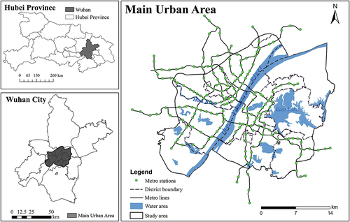
This study focused on the main urban area of Wuhan, which is densely populated, with a large number of dockless shared bikes and high cycling flow, accounting for approximately 88% of the city’s total usage of shared bikes. A total of 708 metro station exits/entrances of 136 different stations alongside eight metro lines were considered, which opened before November 2019 in the main urban area of Wuhan. The bike-sharing dataset collected by Mobike Technology Co., Ltd, the company with the highest market share of dockless bikes in Wuhan, was used. The dataset was generated by bike-sharing orders from November 1 (Friday) to November 7 (Thursday) 2019, a period with good weather conditions and no special events. The dataset contains the position coordinates of order origin and destination, the order start and end time, user ID, and bike ID (Table 1). After data cleaning and deduplication, approximately 0.85 million orders a day on weekdays and 0.73 million a day on weekends were used in this study. It is noteworthy that this study only employed a seven-day dataset, which may not be enough to achieve all the potential of the machine learning techniques, and the statistical and systematical biases in subsequent analysis must be acknowledged. Fortunately, the biases may be diminished due to the periodicity of bike-sharing usage.

Table 1. Example of users’ records.

User_Id	Bike ID	Start-time	O_ longitude	O_ latitude	End-time	D_ longitude	D_ latitude
360550	26628	2019/11/2 20:38	114.4222	30.6058	2019/11/2 20:48	117.2631	34.81315
1012447	65287	2019/11/4 11:57	117.1335	36.6805	2019/11/4 12:11	117.1479	36.68504
980168	70546	2019/11/5 15:11	116.991	36.6689	2019/11/5 15:25	116.9819	36.66227

We also employed demographic and commuting data provided by Baidu, metro station-related data crawled via Gaode map Application Programming Interface, including spatial locations of exits/entrances of each metro station and metro lines, road network and land use data provided by Wuhan Geomatics Institute. The demographic data recorded the Baidu User Density (BUD) in each grid with a spatial resolution of 200 m. Commuting data records the working place and residence of people aged 16–64 with stable commuting characteristics (regular movement between working place and residence for two consecutive weeks).

3.2. Rational service scope of metro stations

Previous studies have shown that the average time spent walking is approximately 10 min during the intermodal process of shared bikes and subways at the TOD level (Ibraeva et al. 2020; Lyu, Bertolini, and Pfeffer 2016). Therefore, the area within a 10-min walk around the metro station was regarded as the potential service scope. The lattice fitting method was applied, which is based on the path planning of Gaode map, to reconstruct the rational service scope of each metro station. Concrete steps are as follows:

Step 1: Set starting point. Each exit/entrance of the metro station was set as the starting point, which means that one station could contain multiple starting points.

Step 2: Set target point. Taking the geometric midpoint of the metro station as the center, the pedestrian lattice was set every 50 m to cover a range of 1.2 km around the station (over 10 min of possible walking distance), constructing a 2.4 km point matrix centered on metro stations.

Step 3: Obtain the minimum time consumption. Based on the actual road network whose precision has reached the garden road level within the community, Gaode path planning provides the optimal path between two points. A Python crawler was designed via Gaode map Application Programming Interface to obtain the minimum time consumption of each route from each starting point to the target point.

Step 4: Generate rational service scope of stations. On the basis of the time consumption of the dot matrix, we constructed the space enclosed by the target points whose time consumption was less than 10 min as the rational service scope.

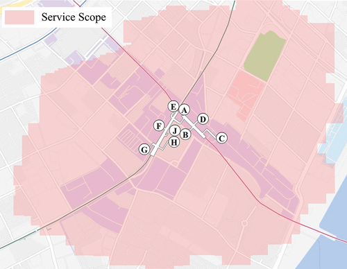
Figure 2 illustrates the service scope as a sample, demonstrating that the service scope generated by path planning based on the real road network is more accurate than that using the traditional GIS method and saves the complex process of constructing a road network.

Figure 2. Schematic diagram of a service scope.

3.3. Definition of the usage patterns of shared bikes

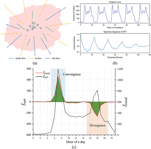
Referring to previous studies, the conceptions of convergence and divergence were introduced to characterize the usage patterns of shared bikes (Yang et al. 2016). The existing dataset contains the location and time information of the start and end points of each bike-sharing order. Therefore, the inside flow of the metro station was defined as the internal activities of sharing bikes and outgoing flow (outflow) as the cumulative departure orders, whereas the incoming flow (inflow) can be defined as the cumulative arrival orders. Figure 3(a) displays the inside flow, outflow and inflow in a designated area during time period $t$. The total flow ($f_{total}$) and net flow ($f_{net}$) can be defined as:

Figure 3. (a) Schematic diagram of inside flow, inflow, and outflow of a station; (b) Workday rhythm of $f_{total}$ and the corresponding spectrum diagrams of FFT; (c) Schematic diagram of convergence-divergence during a day.

(1) $f_{total}=inflow+outflow+inside\hspace{0.17em}flow$(1)

(2) $f_{net}=inflow-outflow$(2)

To describe usage patterns precisely, the $f_{total}$ and $f_{net}$ of each metro station were calculated at intervals of one hour for the week. Considering the significant difference in bike-sharing usage on weekdays and weekends, the spatio-temporal matrix of $f_{total}$ and $f_{net}$ for weekdays and weekends was constructed respectively, as follows:

(3) $F_{total}=\left[\begin{array}{c}{f}_{total}\left[1,1\right],f_{total}\left[1,2\right],\cdots ,f_{total}\left[1,n\right]\\ f_{total}\left[2,1\right],f_{total}\left[2,2\right],\cdots ,f_{total}\left[2,n\right]\\ \dots \\ f_{total}\left[m,1\right],f_{total}\left[m,2\right],\cdots ,f_{total}\left[m,n\right]\end{array}\right]$(3)

(4) $F_{net}=\left[\begin{array}{c}{f}_{net}\left[1,1\right],f_{net}\left[1,2\right],\cdots ,f_{net}\left[1,n\right]\\ f_{net}\left[2,1\right],f_{net}\left[2,2\right],\cdots ,f_{net}\left[2,n\right]\\ \dots \\ f_{net}\left[m,1\right],f_{net}\left[m,2\right],\cdots ,f_{net}\left[m,n\right]\end{array}\right]$(4)

where $n$ represents the length of the time period, 120 (24 × 5) on weekdays and 48 (24 × 2) on weekends; $m$ represents the number of metro stations, which is 136. Before cluster analysis, we tested the periodicity of the time series because the stability of the high-dimensional matrix of the $F_{total}$ and $F_{net}$ time series data has a great impact on the subsequent clustering results. Additionally, the dimension can be reduced by determining the minimum period of the time series. A Fast Fourier Transform (FFT) was applied to conduct the periodic test. FFT is a method of converting time series from the time domain to the frequency domain to determine the period, which is widely used in time series data processing (Lin and Ye 2019). Figure 3(b) shows the origin wave and spectrum diagrams of $F_{total}$ on weekdays as an example, and the main periodic component corresponding to the maximum peak spectrum is 24, which is the period. The results showed that the period of $F_{total}$ at all stations is 24, whereas the period of $F_{net}$ at 94% of stations was 24. The stable periodicity means that we could add and average the time series with a period of 24 h to achieve the purposes of dimensionality reduction and facilitating analysis. Figure 3(c) illustrates the convergence and divergence in a day represented by $F_{total}$ and $F_{net}$, which is also the data basis for the subsequent usage pattern analysis.

3.4. Factors affecting the usage patterns of shared bikes

According to previous studies, four main categories of factors (station attributes, demographics, traffic conditions, and land use variables) were selected to explore the possible relationship with the usage patterns of shared bikes (Ji et al. 2020; Tan et al. 2021; Tu et al. 2021), which are shown in Table 2. Although the socioeconomic attributes of individuals were unavailable due to user privacy, considering that the main users in this study are young people who commute by shared bikes, the economic and social backgrounds may be similar. Therefore, this study mainly focused on the built environment, station attributes, and other macro factors (Zhao and Cao 2020). Betweenness centrality reflects the importance of the station in the metro network, which can replace dummy locational variables, such as “terminal station” and “transfer station,” with a specific value. Betweenness centrality is computed as the number of links between any other two stations passing through station (An et al. 2019), the formula of which is as follows:

Table 2. Factors and collinearity diagnosis.

Variable	Name	Mean	St. dev.	VIF
Station attributes	Number of entrances	5.21	2.59	1.16
	Average distance of the nearest four stations (m)	1546.82	501.59	2.03
	Betweenness centrality	0.07	0.06	1.90
Demographics	BUD (per km^2)	6780.09	4011.18	6.11
	Resident density (per km^2)	2774.37	1579.63	4.12
	Employment density (per km^2)	3803.95	2883.24	5.18
	Job–housing ratio	1.85	2.03	1.94
Traffic conditions	Road density (km/km^2)	10.11	5.64	4.93
	Intersection density (per km^2)	11.23	7.42	4.09
	Bus station density (per km^2)	15.86	6.90	2.19
Land use variables	Shop density (per km^2)	6.61	5.70	5.63
	Living service facility density (per km^2)	60.09	55.78	5.57
	Commercial floor area ratio (%)	91.43	79.30	1.46
	Land use mix	0.60	0.11	1.58

(5) $C_i^B=\frac{1}{\left(N-1\right)\left(N-2\right)}{\sum }_{j=1;k=1;j\ne k\ne i}^N\frac{n_{jk}\left(i\right)}{n_{jk}}$(5)

where $n_{jk}$ represents the number of paths between two stations $j$ and $k$, and $n_{jk}\left(i\right)$ represents the number of paths that contain station $i$. A metro station with a large betweenness may be a transfer station or have a strong connection with other stations in the metro network, whereas the betweenness levels of terminals are mostly close to 0. The BUD social media data in this study are collected from Baidu, the largest Internet company with numerous active users in China, which has been proven to be an effective substitute for reflecting real-time population dynamics and regional vitality (Li et al. 2021). Residential and employment densities were determined by the commuting data provided by Baidu. Due to the spatial separation between jobs and housing and functional group planning, there are obvious boundaries between place of employment and residence in Wuhan. The long-term and stable commuter flow data can reflect the characteristics of regional employment and residence (Cai et al. 2020). All big data are based on a 200 m grid. We used the 2018 building survey data provided by Wuhan Geomatics Institute in using the entropy index ($E{I}_i$) to indicate land use mix:

(6) $E{I}_i=-{\sum }_{k=1}^S{p}_{k,i}\mathrm{l}\mathrm{n}\left(p_{k,i}\right)/\mathrm{l}\mathrm{n}S$(6)

where $S$ is the number of land use types within the scope of station $i$, and $p_{k,i}$ represents the proportion of land use type $k$. A high $EI$ value reflects a diverse land use combination, whereas a close-to-0 value means a single type of land use.

Although the machine learning model can weaken the influence of collinearity through multiple trainings, if the focus is given to the interpretability of the model, then the selection of highly correlated variables is inappropriate because of the substitutability between them (Friedman 2001). Therefore, the Variance Inflation Factor (VIF) was calculated to check for collinearity among the variables. In general, variables with VIF values greater than seven may have multicollinearity and need to be removed from the model (Tang et al. 2019). As shown in Table 2, the VIF values of all variables are below 7, indicating a minimal influence of multicollinearity.

3.5. Model

3.5.1. K-medoids with DTW distance

3.5.1.1. DTW distance

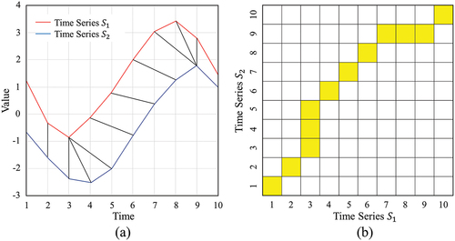
DTW was first introduced for speech recognition and is widely used in pattern mining for time series data (Kate 2015). To cluster the usage patterns represented by $f_{total}$ and $f_{net}$ time series, we used DTW to obtain the “distance” which can better match the peaks and troughs of different time series than Euclidean distance. As illustrated in Figure 4, Euclidean distance uses a one-to-one alignment, whereas DTW distance uses a one-to-many alignment, which means DTW distance can minimize the distance by warping the time dimension, efficiently solving the offset of time series. Suppose two time series $S_1$ and $S_2$ have lengths a and b, respectively. The square of Euclidean distance between any two elements in $S_1$ and $S_2$ was calculated to create a × b distance matrix $D$. A warping path $P$ through matrix $D$ is a series of matrix elements mapped between $S_1$ and $S_2$, which must meet the following three constraints (Javed et al. 2019):

Figure 4. Illustration of DTW distance: (a) Optimal path (black) between time series $S_1$ (red) and time series $S_2$ (blue); (b) a distance matrix showing the process of finding the optimal path and the DTW distance is the sum of distances (orange).

First:

Boundary condition. The first and last points of $S_1$ and $S_2$ must align respectively, which means the beginning and ending of the warping path must be at the diagonally opposite corner cells.

Second:

Continuity. The warping path can only be aligned with adjacent points, and cross-alignment is not allowed.

Third:

Monotonicity. Each point of $S_1$ must be matched to one or more points of $S_2$ and vice versa. Backward matching is not allowed.

DTW distance is the path among all the warping paths that minimize the following equation:

(7) $\mathrm{D}\mathrm{T}\mathrm{W}\left(S_1,S_2\right)=\underset{P\mathrm{b}\mathrm{e}\mathrm{t}\mathrm{w}\mathrm{e}\mathrm{e}\mathrm{n}{S}_1\mathrm{a}\mathrm{n}\mathrm{d}{S}_2}{min}\sqrt{{\sum }_{\left(i,j\right)\equiv p_k\in P}D\left[i,j\right]}$(7)

where $D\left[i,j\right]$ represents the Euclidean distance between the $i$th point of $S_1$ and the $j$th point of $S_2$, obtained by the formula:

(8) $D\left[i,j\right]=d{\left(S_{1i},S_{2j}\right)}^2$(8)

DTW has two variants considering bivariate time series: DTW-independent, which adds the distances that are obtained separately for a single variable, and DTW-dependent that processes $S_1$ and $S_2$ as multivariate time series and only calls DTW algorithm once. Given the importance of the dependency between $f_{total}$ and $f_{net}$, we used DTW-dependent in this study.

3.5.1.2. K-medoids clustering algorithm

K-medoids cluster method is a variant of K-means, which uses actual data points as the cluster centroids. Given that the K-medoids method is based on the representative points located in the clustering centers, it is less sensitive to noise points and outliers compared with K-means (Park and Jun 2009). Besides, compared with other clustering algorithms, K-medoids is applicable to multivariate series. It is an iterative method, and the specific steps are as follows:

First:

Determine the number of clusters k and then randomly select initial centroids from the dataset.

Second:

Calculate the distance from all the points to each centroid. In this study, DTW distance is used, and then all the points are assigned to the closest centroid.

Third:

Select the point with the minimum sum of distances from it to all the other sample points in the cluster as the new centroid.

Fourth:

Repeat the algorithm until the centroid selection is no longer changed.

Hopkins test statistic was used to measure the cluster validity of a dataset. Under the null hypothesis that data are uniformly randomly distributed, Hopkins test statistic can judge the randomness of data in space and further evaluate whether the data can be clustered (Javed et al. 2019). A value of Hopkins test statistic close to 1 means the data is highly clusterable, while a value close to 0.5 implies randomness.

The silhouette coefficient and the Sum of Square Errors (SSE) were chosen to evaluate the clustering result. The silhouette coefficient can measure the cohesion and separation of clustering results to quantificationally represent cluster quality (Rousseeuw 1987), which can be calculated as follows:

(9) $s^{\left(i\right)}=\frac{b^{\left(i\right)}-a^{\left(i\right)}}{max\left\{b^{(i)},a^{(i)}\right\}}$(9)

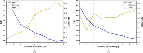
where $a^{\left(i\right)}$ represents the cohesion, which is the average distance between point $i$ and other points in the cluster; $b^{\left(i\right)}$ represents the separation, which is the average distance between point $i$ and all points of other clusters. The closer $s^{\left(i\right)}$ is to 1, the better the performance of the clustering result. We used the elbow method to determine the “optimal” number of clusters k, which means the optimal k is the point where the silhouette coefficient stops sharp increase and SSE stops sharp fall, adding the number of clusters results in diminishing the improvement of the clustering result. Meanwhile, we validated the optimal k value by using the Kneedle algorithm (Satopaa et al. 2011).

3.5.2. Multiclass explainable boosting machine

This study applied a machine learning method named Multiclass Explainable Boosting Machine (MC-EBM), which explores the interpretability of multi-classification. Recently, machine learning models have been widely used in the field of traffic behavior because of their reliable identification of the relative importance of features and potential nonlinear effects (Tao et al. 2020). Compared with traditional multiple logistic regression and other linear models, machine learning models handle multicollinearity well, offer a precise prediction, and do not follow any pre-assumptions (Chen and Ye 2021). Interpretable models, as a form of machine learning method, although occasionally less accurate than blackbox models, are more widely preferred because their transparency helps discover potential relationships among variables (Mi, Li, and Zhou 2020). Explainable Boosting Machine (EBM) is one of the most widely used interpretable models.

EBM is based on Generalized Additive Models plus interaction (GA² M) and can detect the pairwise interactions among input features (Lou et al. 2013), the form of which is:

(10) $g\left(E\left[y\right]\right)={\beta }_0+\sum f_i\left(x_i\right)+\sum f_{ij}\left(x_i,x_j\right)$(10)

where $\sum f_i\left(x_i\right)$ is the individual function term that models the relationship between input feature $x_i$ and output $y$ through link function $g$; $\sum f_{ij}\left(x_i,x_j\right)$ is the pairwise interaction function term that models the relationship between two features $x_i$, $x_j$ and output $g\left(E\left[y\right]\right)$; ${\beta }_0$ is the intercept adjusting the model prediction. MC-EBM generalizes EBM to the multiclass setting and introduces an Additive Post-Processing for Interpretability (API) method to achieve interpretability without sacrificing accuracy (Zhang et al. 2019). MC-EBM satisfies two axioms of interpretability to avoid visual misleading, which is also the design concept of API.

First is the axiom of monotonicity. For each shape function of feature, its monotonicity for all classes should be consistent with the monotonicity of the real prediction probability. Researchers do not want to see a shape function increasing, but the prediction probability is actually decreasing. The second is the axiom of smoothness. For each shape function of feature, it must avoid any unnecessary or artificial unevenness. The discontinuities of shape function make it difficult to understand the prediction trend. On this premise, MC-EBM can generate the shape functions of each feature on each class to illustrate the changes in the influence at different values of the feature.

Some limitations should be noticed. First, MC-EBM cannot provide the confidence intervals of coefficients. However, this study emphasized the practical significance of variables and weakened their statistical inferential significance. Second, similar to other machine learning models, MC-EBM has the possibility of overfitting. Hence, we used the fivefold cross-validation method and balance classification test dataset to reduce the impact of overfitting. Last, some fluctuations may occur in the intervals with few samples. Thus, we combined the distributions of samples and analysis cautiously in unreliable estimation intervals.

4. Results

4.1. Usage patterns of shared bikes at the TOD level

The Hopkins test statistic of the bike-sharing dataset on weekdays was 0.84 and on weekends was 0.86, indicating a highly clusterable characteristic (Banerjee and Dave 2004). Using both the elbow method and the Kneedle algorithm, it was determined that the clustering numbers were 6 and 4 on weekdays and weekends, respectively, when K-medoids were applied with DTW-dependent to the dataset (Figure 5).

Figure 5. SSE and silhouette for different numbers of clusters (a) on weekdays (the elbow is at 6.) and (b) on weekends (the elbow is at 4.).

4.1.1. Usage patterns on weekdays

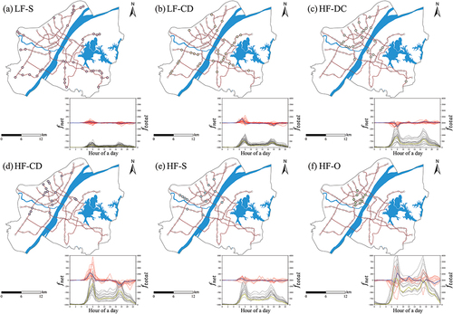
Table 3 shows the names and proportions of different usage patterns, and two segments were used to represent the name of each pattern according to their riding intensity and convergence-divergence characteristics. The riding intensity was divided into high total flow and low total flow, which are abbreviated as HF and LF respectively. Four types of convergence-divergence characteristics were identified: all-day stability (S), convergence in the morning and divergence in the evening (CD), divergence in the morning and convergence in the evening (DC), and all-day oscillation (O).

Table 3. Usage patterns for weekdays and weekends.

Clusters	LF-S	LF-CD	HF-DC	HF-CD	HF-S	HF-O
Weekdays	30.88%	22.79%	16.18%	13.24%	9.56%	7.35%
Weekends	55.15%	18.38%	-	18.38%	-	8.09%

The statistical results and spatial distribution of the six patterns for weekdays are shown in Figure 6. The hourly profiles of $f_{total}$ and $f_{net}$ were also plotted for different patterns in which the clustering centers are highlighted by a yellow line ($f_{total}$) and a blue line ($f_{net}$). The proportion of LF-S pattern was 30.88%, which was the dominant type with a stable and low riding flow. No obvious peaks or troughs were found in the curve, indicating a random use of shared bikes. Spatially, LF-S pattern was mainly distributed at the edge of the main urban area with a sparse population where the commuting demand was low and the intensity of daily activities was weak. LF-CD pattern, with a proportion of 22.79%, witnessed inconspicuous tidal patterns where the shared bikes converged in the morning rush hours and diverged in evening rush hours at a relatively low $f_{total}$ level. HF-DC pattern, with a proportion of 16.18%, was the opposite in the pattern of convergence and divergence. Stations with LF-CD pattern were mainly distributed in the residential communities near the Second Ring Road. In contrast, stations with HF-DC pattern were close to the urban center. This intuitively shows that sharing bikes as a connection tool solves the first/last mile problem. Numerous residents go to the metro stations by bike to commute in the morning and leave the metro stations in the evening, causing the accumulation and dispersion of shared bikes in the morning and evening peaks, respectively. Near the workplace, the opposite was true because more commuters ride from subway stations to workplaces during the morning peak, which caused the divergence of shared bikes. The peak value of the $f_{net}$ curve in the evening rush time was lower than that in the morning rush time. It is plausible that commuters need to save time in the morning to catch up with the company’s time regulations, while the choice of transportation modes after work was more diverse because there was no need to consider the time cost too much. The proportion of HF-CD pattern was 13.24%, and its tidal phenomenon was considerably obvious where shared bikes converged in the morning peak and diverged in the evening peak. The peak and trough of the $f_{net}$ curve were formed quickly, and the duration was approximately three hours. Stations with HF-CD pattern were distributed near the city center where residential and employment activities were relatively intensive. Bike-sharing travels in these areas were generally for the purpose of commuting on weekdays. The proportion of HF-S pattern was 9.56%, and its $f_{total}$ value was relatively high, whereas its $f_{net}$ curve was steady overall, and the fluctuation does not have an obvious peak timing. Most areas with HF-S pattern were mixed business districts, and the purpose of sharing bikes was diverse. The proportion of HF-O pattern was 7.35%, and its $f_{total}$ value was the highest among all clusters. The fluctuation of the $f_{net}$ curve was obvious all day, not only in the morning and evening commuting peaks. HF-O pattern was concentrated in the urban center with high mixed land use types where the intensity of human activities was fairly high, whereas human mobility does not show a consistent pattern on the time scale.

Figure 6. Metro station distribution of different patterns and corresponding hourly profiles of $f_{total}$ (black) and $f_{net}$ (red) on weekdays.

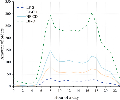
The inside flow of each usage pattern was counted separately to find the internal use of shared bikes, which may not be related to the connection to metro station. Figure 7 shows the average hourly inside flow of six usage patterns for weekdays. Overall, the distribution of inside flow and total flow is similar in time, but the inside flow of HF-CD pattern and HF-O pattern in the morning and evening peak are significantly higher than that of the other four types. Combined with the spatial distribution, these two usage patterns are distributed closer to the urban center and have a higher degree of mixing of work and residence. Therefore, the shorter trips with shared bikes as the direct commuting mode is more likely to occur in the morning and evening peak. Besides, the “lunch spike” appears in these two patterns at 12 noon, which also shows that the mix of land functions in the urban center makes some short-distance use of shared bikes for non-commuting purposes on weekdays. In addition, due to the large number of bike-sharing usage for shorter trips and the agglomeration of metro station in the downtown area, the $f_{net}$ value of HF-O pattern fluctuates greatly throughout the day.

Figure 7. Hourly fluctuation of inside flow in different patterns on weekdays.

4.1.2. Usage patterns on weekends

Figure 8 shows the hourly profiles and spatial distribution of the four patterns for weekends. As the weekend riding demand was less than that on weekdays, the usage patterns were less, and the tidal phenomenon in the morning and evening peaks was not obvious. Additional stations were classified into LF-S pattern, with a proportion of 55.15%, and the $f_{total}$ value of some stations was close to 0. The proportion of LF-CD pattern was 18.38%, and the peaks and troughs of the morning and evening peaks in LF-CD pattern almost disappeared. Instead, the change in $f_{total}$ value from 7:00 to 19:00 was also stable, which means that as the commuter flows attenuate, the peak demand for shared bikes decreases. The third usage pattern was similar to HF-CD pattern on weekdays, with a proportion of 18.38%. Even on weekends, convergence still occurred in the morning and divergence at night, and the occurrence time of divergence of some stations was postponed to approximately 20:00. The fourth usage pattern was similar to HF-O pattern on weekdays, with a proportion of 8.09%. These stations maintain high riding intensity.

Figure 8. Metro station distribution of different patterns and corresponding hourly profiles of $f_{total}$ (black) and $f_{net}$ (red) on weekends.

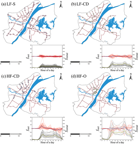
Spatially, the use of shared bikes further shrinked to the urban center, with larger spatial differentiation than the suburbs. The spatial autocorrelation for the usage patterns on weekdays and weekends was also tested by using Moran’s I index in ArcGIS software. The p-value on weekdays was not significant, and the Z-score was 0.5, which means that the usage patterns presented a random distribution in space. In contrast, the p-value on weekends was lower than 0.01 and the Z-score was 11.5, which denotes that the usage patterns were spatially clustered. Stations with tidal phenomena were mostly near the urban center with intensive employment, whereas stations with high riding intensity were still in the urban center.

Figure 9 shows the inside flow of four usage patterns for weekends. The total amount of inside flow of shared bikes is considerably lower than that on weekdays, and the gap between HF-O pattern and other patterns is more obvious, indicating a more concentrated use of shared bikes in the urban center on weekends. Without the pressure of work schedule, people tend to casually use shared bikes, which makes the peak value of morning and evening rush time of the curve smaller, but also leads to the disorder of the fluctuation of $f_{net}$ value throughout the day, especially HF-O pattern.

Figure 9. Hourly fluctuation of inside flow in different patterns on weekends.

4.2. Influential factors of the usage patterns of shared bikes

Different combinations of hyperparameters were tested by using a fivefold cross-validation method to obtain the optimal parameter settings and improved results. As an imbalanced classification dataset, synthetic minority oversampling and cleaning undersampling were also combined to build a balanced test set of expanded samples. To avoid the optimistic estimate caused by biased classifiers on imbalanced datasets, the balanced accuracy metric was used to measure the performance, which can better evaluate the model in classification tasks considering the imbalance of classes (Zhang et al. 2019):

(11) $BACC\left(f\right)=\frac{1}{K}{\sum }_{k=1}^K\mathrm{P}\left(f\left(\mathbf{x}\right)=k\mid y=k\right)$(11)

Finally, the balanced accuracies of the training and test sets on weekdays were 0.91 and 0.88 and those on weekends were 0.84 and 0.79, respectively. Considering the small difference between the training and test sets, the influence of overfitting may be relatively small. The weekday and weekend models achieve satisfactory accuracy, showing considerable performance.

After standardizing each variable, the results on weekdays were compared with the Multiclass Logistic Regression (MLR) model, which is universally used to predict the probabilities of different possible results for the dependent variables. In general, a base class should be designated in MLR, and the interpretation of other classes is based on the comparisons of the base class. LF-S pattern was selected as the base class because it was the most common pattern. The model was significant with a confidence level of 0.001, suggesting that the model was valid. Nagelkerke’s R² and balanced accuracy were 0.86 and 0.71, respectively, indicating a good explanation. Unsurprisingly, the predictive accuracy was lower than that of the MC-EBM model because capturing the nonlinear effects promotes the overall goodness-of-fit. In addition, the MLR model cannot effectively reveal the transformation among all possible classes because of the preset base classes.

4.2.1. Relative importance of explanatory variables

Relative importance was a widely used method of interpretable models, measured by the times a certain feature was selected and that of all features adds up to 100% (Tao et al. 2020). A feature with high relative importance can make a large contribution to the prediction. Table 4 presents the relative importance of explanatory variables in influencing the usage patterns of shared bikes on weekdays and weekends. The most influential category of variables was demographic. Demographic characteristics represent activity intensity and job-residence relationships, which often spatially and temporally affect travel behavior, both on weekdays and weekends. While traffic conditions have a greater impact on weekends than on weekdays, people prefer to use shared bikes in regions with good traffic conditions, given the flexibility and freedom of weekend travel behavior (Li et al. 2020).

Table 4. Relative importance of variables.

Variable	Weekday		Weekend
	Relative importance (%)	Rank	Relative importance (%)	Rank
Station attributes	19.92		19.42
Number of entrances	7.62	5	6.49	10
Average distance of the nearest four stations	8.42	2	9.22	2
Betweenness centrality	3.88	14	3.71	14
Demographics	29.96		27.96
BUD	6.84	11	7.37	9
Resident density	7.40	6	7.79	6
Employment density	7.39	7	9.04	3
Job–housing ratio	8.33	3	3.76	13
Traffic conditions	23.78		27.15
Road density	9.50	1	10.69	1
Intersection density	7.04	10	8.90	4
Bus station density	7.24	8	7.56	8
Land use variables	26.34		25.47
Shop density	7.14	9	7.65	7
Living service facility density	7.80	4	8.36	5
Commercial floor area ratio	5.59	13	4.13	12
Land use mix	5.82	12	5.32	11

In terms of single variables, road density and the average distance of the nearest four stations were the two most important variables, whereas betweenness centrality was the least important on weekdays and weekends. These findings imply that compared with the location in the metro network, the density of the metro station plays a more important role in affecting travel behavior (Lin et al. 2019). Among the land use variables, the impact of a single variable may seem trivial, but combining multiple land use variables can achieve a larger impact.

4.2.2. Associations between key variables and usage patterns on weekdays

Partial Dependence Plots (PDPs) were used to visualize the marginal effects of variables on the predicted outcomes, given that all other variables remained constant. PDPs show the probability of each usage pattern when the variable takes different values. The probability curve of each usage pattern was drawn in the form of ladder diagrams to avoid the excessive fluctuation of the curve. Meanwhile, the density distribution of each explanatory variable was drawn below the possibility graph, where a higher density means more data points and the results tend to be more reliable. The fluctuation caused by the sparse data density should be carefully interpreted.

Considering the complex causes of tidal stations, PDPs were marked with different line types, solid lines for clusters with tidal phenomena (LF-CD, HF-DC, and HF-CD) and dotted lines for clusters without the tidal phenomena (LF-S, HF-S, and HF-O). Among them, HF-S pattern achieves dynamic balance while maintaining high riding vitality, which greatly reduces the occurrence of tidal flow problems. Therefore, increasing the probability of HF-S pattern is more conducive to the efficient operation of the bike-sharing system, improving commuting efficiency and satisfaction of bike-sharing users.

As illustrated in Figure 10(a), LF-S pattern likely occurs in regions with low road density, and more precisely, the road density was less than 10.3 km/km². LF-S pattern represents the suburbs with low riding vitality, which generally have low population density and public facility density. While a high road density can create a convenient riding environment and stimulate riding demand, this impact seems to be weakened when road density exceeds 14 km/km². At this time, HF-CD and HF-O likely occur, and HF-O pattern becomes the dominant pattern in areas with road densities greater than 20 km/km². In terms of clusters with tidal phenomena, LF-CD and HF-DC patterns are less affected by road density, whereas HF-CD pattern most likely occurs in the range of 10.3–20 km/km², and the probability peaks at approximately 12 km/km².

Figure 10. Nonlinear associations between the top five key variables and usage patterns on weekdays.

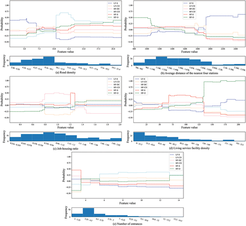
Figure 10(b) indicates a similar trend, which was reasonable because the average distance of the surrounding stations reflects the station density. The higher the density of metro stations is, the greater the human mobility and activity intensity because of the convenience of travel. Additionally, as a time-saving approach of arriving/departing the subway station, the use of shared bikes was also significantly affected by the station density, especially when it was below the threshold of 1915 km. At tidal stations, HF-DC and HF-CD patterns were less affected, whereas the probability of LF-CD pattern increases first and then decreases, peaking at approximately 1800 km.

The balanced job – housing space was generally believed to be the region with a job – housing ratio between 0.8 and 1.3 (Lin, Allan, and Cui 2016). Figure 10(c) illustrates that LF-CD pattern was the dominant type in the balanced job – housing regions, whereas HF-DC pattern likely occurs in regions with a low job – housing ratio, and the turning point was approximately 1.21. On weekday mornings, scenarios where shared bikes flow out in residential-dominated areas but flow in work-dominated areas were reasonable because of commuting activities (Fishman 2015). When the job – housing ratio was between 1.21 and 1.30, the probability of HF-S pattern has a short peak, indicating that the job – housing balance may contribute to the dynamic load balancing of shared bikes.

As the living service facility density becomes high, an increased probability of HF-O pattern and a decreased probability of other clusters were observed, except for HF-S pattern in Figure 10(d). The curve of HF-S pattern presents an inverted U, which means that a moderate-scale living facility configuration may be conducive to creating users of shared bikes while stabilizing $f_{net}$ value.

For the number of entrances, HF-S pattern most likely appears when it was lower than 4 (Figure 10(e)). With the increase in the number, HF-CD pattern gradually becomes the dominant pattern. Note that the curve may be less reliable in the ranges above 12, owing to the absence of enough sample data. At stations with more entrances, tidal patterns that converge in the morning and diverge at night are more likely to occur. A situation where more entrances may attract more commuters is reasonable, resulting in tidal patterns of the usage of shared bikes.

4.2.3. Associations between key variables and usage patterns on weekends

As illustrated in Figure 11(a), the overall trend was consistent with that on weekdays, whereas for stations with tidal phenomena, it most likely occurs in a smaller road density range of 10.2–13.0 km/km². Similarly, the effective influence interval of the average distance of the surrounding stations shrinks to 1730 km, as displayed in Figure 11(b). This occurrence was understandable because the area covered by bike-sharing travel on weekends was small, which means that the change in environmental variables was limited (Li et al. 2020).

Figure 11. Nonlinear associations between the top five key variables and usage patterns on weekends.

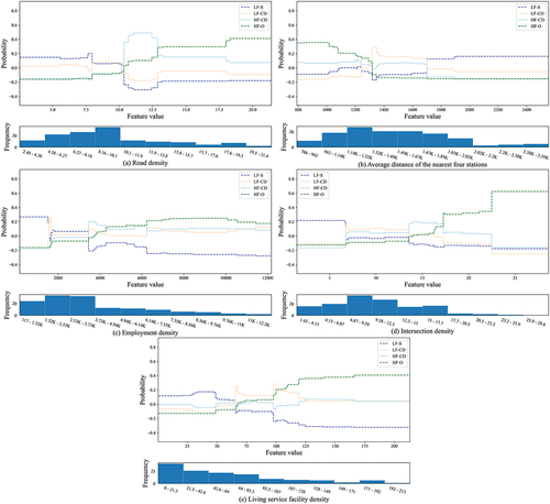
Employment density was the third important variable, which has a considerable impact not only on LF-S and HF-O but also on HF-CD in the interval with sufficient training data, as illustrated in Figure 11(c). Even on weekends, some Internet and financial companies still maintain commuting hours on weekdays, resulting in tidal phenomena. This impact was most obvious in areas with an employment density range of 3450–6100 per km².

Figure 11(d) shows that intersection density has a strong impact on promoting the use of shared bikes where the probability of HF-O pattern was higher than that of other classes after the intersection density reaches 17 per km². A higher intersection density around metro stops means better network connectivity, providing more alternative routes, which may increase users’ willingness to ride (Liu, Wang, and Xiao 2021). In addition, the tidal phenomenon may occur at a high intersection density, precisely in the range of 14–17 per km². Figure 11(e) indicates that the effect of stabilizing $f_{net}$ value in a medium living facility market is also effective on weekends, which has an effective range of 65–100 per km².

5. Discussion

5.1. Comparison of usage patterns on weekdays and weekends

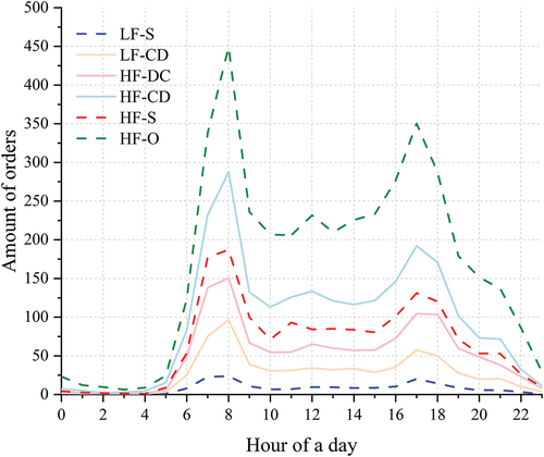
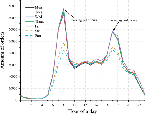
We also summed the bike-sharing orders within the reconstructed service scope of all metro stations every day of the week (Figure 12). The usage of shared bikes in Wuhan is quite distinct at different times of the day, as well as on weekdays and weekends. The usage curves on weekdays show two commuting peaks in the morning and evening, which means that a large number of orders suddenly appear around the metro stations, indicating that shared bikes are widely used as a transfer tool to facilitate first/last mile connection to public transport during commute times. The morning peak usage is higher than the evening peak, which is different from previous studies (Li et al. 2020), suggesting an increased usage for commuting purposes in Wuhan, whereas the usage of shared bikes is reduced after work because of the increase in recreational travel. On weekends, the morning and evening peaks almost disappear, and a secondary peak at approximately 21:00 implies that outdoor leisure or social activities may become mainstream. Compared with studies in Paris (Kabra, Belavina, and Girotra 2020), in which the time when usage peak appears is in the afternoon, and research in Nice shows no remarkable differences between weekdays and weekends (O’Brien, Cheshire, and Batty 2014), the different results may be due to the different rhythms of working-life style, which also implies that shared bikes are more a tool for connecting public transport for commuting in Wuhan.

Figure 12. Hourly fluctuation of bike-sharing demand per day.

As the regions with the most frequent activities of residents in the city, some non-commuting trips are often carried out by shared bikes near metro stations. Shared bikes are also used as direct transportation for short commuting as an alternative to walking. Generally, the travel distance would be shorter if the purpose of using shared bikes is leisure activities (Li, Zhu, and Guo 2019). We compared the mean trip length with other studies conducted outside Wuhan. According to the studies from Shanghai and Beijing, the mean trip lengths are 1.32 km and 1.45 km respectively (Lin et al. 2019; Wang, Chen, and Xu 2016), which are shorter than the average distance of 1.71 km obtained in this paper. Due to the “commuting desert” caused by the group planning in some regions, commuters in Wuhan are relatively dependent on public transport (Cai et al. 2020). Therefore, it is reasonable that more long-distance trips are observed, which the shared bikes are more likely to be used to connect to the metro stations. In addition, compared with the bus, the service capacity of the subway is stronger, and the parking of shared bikes is often prohibited near bus stops. Consequently, the connection between shared bikes and subways is significantly more than that of connecting buses, especially in metropolises like Wuhan. Approximately 30% of the orders are under 1 km; hence, incentive measures could be implemented to encourage longer distance riding, thereby promoting the shift from buses to shared bikes, and expanding the influential scope of the metro station.

Furthermore, the usage patterns at the TOD level can be divided into three types: stable type (LF-S, HF-S), tidal type (LF-CD, HF-DC, and HF-CD), and high-flow oscillation type (HF-O). Additional stations are grouped into stable types on weekends because of weekend downtime. The stable type with relatively high riding flow (HF-S) can be regarded as an effective pattern of using shared bikes. For the stable type with low riding flow (LF-S), managers should consider two aspects. On the one hand, the delivery scale in combination with user needs should be further controlled. Although the Wuhan municipal government reduced the total number of shared bikes from 1.03 million in 2018 to 0.58 million by the end of 2019 through multiple rounds of regulation, the problem of excessive delivery remains in some areas, causing a waste of resources. On the other hand, the utilization of shared bikes should be improved. Stations close to residential and commercial areas, especially stations reclassified into stable types due to the weakening of commuting activities on weekends, have certain user market potential (Shen et al. 2020). Fee concessions may be effective in these regions and can hence foster clean and energy-saving travel modes (Parkes et al. 2013). The spatial position of the high-flow oscillation type is relatively fixed and is located in the central activity area and large business districts. Additional regulations may be needed in these areas.

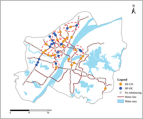
Further attention should be given to tidal types where the nonequilibrium of arrival and departure flows may bring challenges to the scheduling of shared bikes. Fortunately, two opposite tidal patterns exist and some of them are adjacent on weekdays (Figure 13). Based on the spatial distribution, the rebalancing strategy can be optimally paired to schedule the stock of shared bikes among stations with opposite tidal patterns to dynamically alleviate the problems caused by the tidal phenomenon. With the shortest distance cost, the shared bikes accumulated in stations with HF-CD pattern can be transferred to stations with HF-DC pattern in the morning peak hours, and the opposite measures can be taken in the evening peak hours, so as to rebalance the number of shared bikes. For nonequilibrium stations on weekdays, some recreational travel may compete with commuting travel for the use of shared bikes. Thus, introducing price incentives to limit recreational use can mitigate fleet imbalance, which has been proven effective (Fishman 2015). The spatio-temporal distribution pattern of tidal type revealed in this study can provide a reference for the rebalancing plans of bike-sharing operators.

Figure 13. Dynamic rebalancing zones adjacent to HF-CD pattern and HF-DC pattern inside the red ellipse.

5.2. Key factors affecting the usage patterns of shared bikes

The modeling results show that the two most important variables are road density and the average distance of the surrounding stations on weekdays and weekends, both of which are different from previous studies that consider population to be the most decisive factor affecting the usage of shared bikes (Du, Deng, and Liao 2019; Tan et al. 2021). The population may have significant effects when differentiating high flows from low flows, while the impact may be inelastic when considering net flows based on a time series model, whereas built environment variables play a greater role in influencing use patterns. Betweenness centrality is the least important, which suggests that when implementing the TOD policy, the focus should be shifted from network nodes to high station density areas. The rankings of shop density and commercial floor area ratio increase, whereas the ranking of job – housing ratio decreases on weekends, indicating an increase in the recreational use of shared bikes, which is consistent with previous studies (Fishman 2015; Li et al. 2020). In terms of each category of variables, road density, living service facility density and resident density are the main influencing factors on both weekdays and weekends, which can be understood that the comprehensive impact of built-up environment attraction, facility suitability and riding demand leads to the different usage patterns. The management strategy considering these factors is the key to maintaining the even distribution and dynamic balancing use of shared bikes.

Nonlinear effects challenge the linearity assumption, providing some meaningful supplements when exploring the relationship between variables and usage patterns. Most variables have thresholds and some variables have associations of inverted U shape with tidal patterns, indicating that stations with tidal phenomena likely occur in some specific value ranges, which may inform operators with a refined effective range to implement strategies and prioritize intervention resources. For example, the probability of HF-CD pattern is the lowest when the road density is less than 10.3 km/km². While the probability increases sharply and exceeds all other patterns in the range of 10.3–13.0 km/km², which means that the tidal flow of shared bikes in these regions is very obvious. More attention should be paid to the accumulation of shared bikes in the morning and insufficient supply in the evening rush time. Similarly, when the range of living service facility density is from 65 to 130 per km², the probability of HF-S pattern exceeds all other patterns, which means the moderate configuration of resources such as shops and living services may be conducive to promoting the balancing use of shared bikes. In addition, high road density can increase the possibility of HF-O pattern both on weekdays and weekends, but the slope becomes small and the effect seems trivial beyond 13.0 km/km². This threshold suggests that the densification strategy may facilitate the use of shared bikes but has a diminishing return.

For bike-sharing companies, the dynamic balance of bike-sharing usage requires flexible delivery and scheduling strategies. Combined with the nonlinear influence of key variables, bike-sharing operators can adopt different block dispatching strategies according to the scale of residential areas and employment areas, the facility suitability, and regional riding conditions. In small residential communities with weak user bases, bike-sharing companies can offer higher discounts to mine potential uses. While in areas with better built environment and more users, more emphasis should be put on the management of bike-sharing flow fluctuation. In addition, when road density is in the range of 10.3–13.0 km/km² and the job-housing ratio is less than 1.21, the probability of tidal patterns is much higher than that of other patterns, so the operators should pay more attention to the rebalancing of shared bikes in these regions. For policymakers, the obtained variable threshold of HF-S pattern also provides a reference for TOD planning from the perspective of building a riding-friendly environment. Policymakers can increase the scale of residential communities and ensure the completeness of supporting facilities. Meanwhile, promote the balance between regional residence and employment, and avoid excessive job-housing separation. Smoothing break road sections and optimizing the medium and low-density road network to construct multi-level road networks suitable for riding. In particular, the densification strategy has a corresponding threshold, such as 1.3 of job-housing ratio and 13.0 km/km² of road density.

6. Conclusions

This work investigated the spatio-temporal patterns of the usage of dockless shared bikes and further explored the nonlinear effects of possible factors influencing the usage patterns at the TOD level. The rational service scope of metro stations was reconstructed in line with the TOD concept and derived two measures ($f_{total}$ and $f_{net}$) from the OD data of bike users to present the convergence and divergence at different times of the day. A time series with two variables ($f_{total}$ and $f_{net}$) was generated for each station and clustered stations by using the DTW distance-based K-medoids algorithm. Then, the MC-EBM model was applied to identify key variables and illustrate the threshold and nonlinear effects on each cluster.

Six patterns were found on weekdays and four patterns on weekends, which can be divided into three types. The use of shared bikes was less and further concentrated in the urban center on weekends. Driven by commuting activities, the tidal phenomenon was more obvious on weekdays, whereas the number of stable types was larger on weekends. The identified spatio-temporal patterns and their spatial distribution can guide operators, whether in promoting the use of shared bikes or arranging the rebalancing management schedule of the tidal phenomenon. Some key variables affecting usage patterns on weekdays and weekends were the same, such as road density and the average distance of the nearest four stations, while some are different, such as job – housing ratio on weekdays and employment density on weekends. These quantitative importance levels and rankings may be worthy of reference to prioritize strategies to achieve efficient management of bike-sharing systems and promote TOD policy. The probability of patterns varies in different value ranges, suggesting that the influence of variables was nonlinear. The nonlinear effects and thresholds could inform the effective ranges of built environment adjustment on different patterns and thus provide targeted intervention for TOD practice.

Several limitations merit further explorations. First, the service scope of stations can be extended at multiple scales. Although the 10-min walk was the common concept of TOD, different levels (i.e. 15-min or 20-min walk) to aggregate the data may have different results in which multiscale analysis can bring further detailed guidance (Liu et al. 2020). When multisource datasets at different spatial resolutions are collected at the same level, determining how to reduce the aggregation error was a universal issue (Zhao et al. 2013; Dangermond and Goodchild 2019). Future studies can supplement unified finer-grained big data. Second, the dataset only covers one week. Although the use of shared bikes shows obvious periodicity, more data should be introduced to verify the characteristics of spatio-temporal usage patterns and related influencing factors (Wu, Gui, and Yang 2020). There may be seasonal or weather-related differences in usage patterns, while without the influence of special weather or events, the change in bike-sharing usage is minor. A longer time span of research may require a new framework. In addition, annual variations in usage patterns may reflect changes in the travel behavior of residents and the effects of traffic facility construction. Last, introducing the analysis of time series variables (i.e. hourly population density) and individual attribute variables could be a meaningful supplement to the research to further explain the patterns on the time scale. However, the sociodemographic characteristics or travel attitudes of individuals cannot be extracted due to the desensitization of big data. If individual survey data could be combined in the future, then the results would be more realistic. Furthermore, the results from this case study could be unique and unable to form an effective comparison with relevant cities. The generalizability merits further research. Future works can investigate other cities and compare intercity variations.

Disclosure statement

No potential conflict of interest was reported by the author(s).

Data availability statement

Restrictions apply to the availability of these data. The data are not publicly available due to Mobike’s contract and privacy policy.

Additional information

Funding

This research is supported by the National Key Research and Development Program of China [grant number 2017YFB0503601]

Notes on contributors

Zhaomin Tong

Zhaomin Tong is a PhD candidate in School of Resource and Environmental Science, Wuhan University, China. His research interests include geospatial analysis, spatio-temporal behavior and complex urban system.

Yi Zhu

Yi Zhu is an assistant engineer in Chengdu Land Planning and Cadastral Affairs Center, Chengdu, China. He got his master’s degree from School of Resource and Environmental Science, Wuhan University. His research mainly focuses on spatial quantitative analysis and urban design.

Ziyi Zhang

Ziyi Zhang received the PhD degree from Wuhan University. Her main research interests and publications are on ecological remote sensing.

Rui An

Rui An is a PhD student at School of Resource and Environmental Science, Wuhan University, China. His research interests include land-use modeling, spatial data aggregation and travel behavior. He is also interested in geospatial analysis.

Yaolin Liu

Yaolin Liu is a professor at School of Resource and Environmental Science, Wuhan University, China. He specializes in spatial modeling.

Meng Zheng

Meng Zheng is the director of Wuhan Transportation Development Strategy Institute. His main research interest is sustainable urban transportation.

References

- An, D., X. Tong, K. Liu, and E. H. W. Chan. 2019. “Understanding the Impact of Built Environment on Metro Ridership Using Open Source in Shanghai.” Cities 93: 177–187. doi:10.1016/j.cities.2019.05.013.
- Banerjee, A., and R. N. Dave. 2004. “Validating Clusters Using the Hopkins Statistic.” In Paper presented at the 2004 IEEE International Conference on Fuzzy Systems, Budapest, Hungary, July 25-29. doi: 10.1109/FUZZY.2004.1375706.
- Buck, D., R. Buehler, P. Happ, B. Rawls, P. Chung, and N. Borecki. 2013. “Are Bikeshare Users Different from Regular Cyclists?” Transportation Research Record: Journal of the Transportation Research Board 2387 (1): 112–119. doi:10.3141/2387-13.
- Cai, M., J. Jiao, M. Luo, and Y. Liu. 2020. “Identifying Transit Deserts for Low-Income Commuters in Wuhan Metropolitan Area, China.” Transportation Research Part D: Transport and Environment 82. doi:10.1016/j.trd.2020.102292.
- Capodici, A. E., G. D’Orso, and M. Migliore. 2021. “A GIS-Based Methodology for Evaluating the Increase in Multimodal Transport Between Bicycle and Rail Transport Systems. A Case Study in Palermo.” ISPRS International Journal of Geo-Information 10 (5): 321. doi:10.3390/ijgi10050321.
- Chabchoub, Y., and C. Fricker. 2015. “Classification of the Vélib Stations Using Kmeans, Dynamic Time Warping and DBA Averaging Method.” In Paper presented at the 2014 International Workshop on Computational Intelligence for Multimedia Understanding (IWCIM), Paris, France, November 1-2. doi: 10.1109/IWCIM.2014.7008802.
- Chen, E., and Z. Ye. 2021. “Identifying the Nonlinear Relationship Between Free-Floating Bike Sharing Usage and Built Environment.” Journal of Cleaner Production 280: 124281. doi:10.1016/j.jclepro.2020.124281.
- Dadhich, P. N., and S. Hanaoka. 2012. “Spatial Investigation of the Temporal Urban Form to Assess Impact on Transit Services and Public Transportation Access.” Geo-Spatial Information Science 15 (3): 187–197. doi:10.1080/10095020.2012.715955.
- Dangermond, J., and M. F. Goodchild. 2019. “Building Geospatial Infrastructure.” Geo-Spatial Information Science 23 (1): 1–9. doi:10.1080/10095020.2019.1698274.
- Ding, C., X. Cao, and Y. Wang. 2018. “Synergistic Effects of the Built Environment and Commuting Programs on Commute Mode Choice.” Transportation Research Part A: Policy and Practice 118: 104–118. doi:10.1016/j.tra.2018.08.041.
- Du, Y., F. Deng, and F. Liao. 2019. “A Model Framework for Discovering the Spatio-Temporal Usage Patterns of Public Free-Floating Bike-Sharing System.” Transportation Research Part C: Emerging Technologies 103: 39–55. doi:10.1016/j.trc.2019.04.006.
- Duran-Rodas, D., E. Chaniotakis, and C. Antoniou. 2019. “Built Environment Factors Affecting Bike Sharing Ridership: Data-Driven Approach for Multiple Cities.” Transportation Research Record: Journal of the Transportation Research Board 2673 (12): 55–68. doi:10.1177/0361198119849908.
- Fang, Z., X. Yang, Y. Xu, S.-L. Shaw, and L. Yin. 2017. “Spatiotemporal Model for Assessing the Stability of Urban Human Convergence and Divergence Patterns.” International Journal of Geographical Information Science 31 (11): 2119–2141. doi:10.1080/13658816.2017.1346256.
- Fishman, E. 2015. “Bikeshare: A Review of Recent Literature.” Transport Reviews 36 (1): 92–113. doi:10.1080/01441647.2015.1033036.
- Friedman, J. H. 2001. “Greedy Function Approximation: A Gradient Boosting Machine.” Annals of Statistics 29 (5): 1189–1232. doi:10.1214/aos/1013203451.
- Froehlich, J., J. Neumann, and N. Oliver. 2008. “Measuring the Pulse of the City Through Shared Bicycle Programs.” In Paper presented at the Proceedings of International Workshop on Urban, Community, and Social Applications of Networked Sensing Systems, Raleigh, USA, November 4.
- García-Palomares, J. C., J. Gutiérrez, and M. Latorre. 2012. “Optimizing the Location of Stations in Bike-Sharing Programs: A GIS Approach.” Applied Geography 35 (1–2): 235–246. doi:10.1016/j.apgeog.2012.07.002.
- Hickman, R., and P. Hall. 2008. “Moving the City East: Explorations into Contextual Public Transport-Orientated Development.” Planning Practice and Research 23 (3): 323–339. doi:10.1080/02697450802423583.
- Huang, B., and J. Wang. 2020. “Big Spatial Data for Urban and Environmental Sustainability.” Geo-Spatial Information Science 23 (2): 125–140. doi:10.1080/10095020.2020.1754138.
- Ibraeva, A., G. H. D. A. Correia, C. Silva, and A. P. Antunes. 2020. “Transit-Oriented Development: A Review of Research Achievements and Challenges.” Transportation Research Part A: Policy and Practice 132: 110–130. doi:10.1016/j.tra.2019.10.018.
- Javed, A., S. Hamshaw, D. Rizzo, and B. Lee. 2019. “Analysis of Hydrological and Suspended Sediment Events from Mad River Watershed Using Multivariate Time Series Clustering.” arXiv Preprint arXiv: 1911.12466.
- Ji, Y., X. Ma, M. He, Y. Jin, and Y. Yuan. 2020. “Comparison of Usage Regularity and Its Determinants Between Docked and Dockless Bike-Sharing Systems: A Case Study in Nanjing, China.” Journal of Cleaner Production 255. doi:10.1016/j.jclepro.2020.120110.
- Jiménez, P., M. Nogal, B. Caulfield, and F. Pilla. 2016. “Perceptually Important Points of Mobility Patterns to Characterise Bike Sharing Systems: The Dublin Case.” Journal of Transport Geography 54: 228–239. doi:10.1016/j.jtrangeo.2016.06.010.
- Kabra, A., E. Belavina, and K. Girotra. 2020. “Bike-Share Systems: Accessibility and Availability.” Management Science 66 (9): 3803–3824. doi:10.1287/mnsc.2019.3407.
- Kaltenbrunner, A., R. Meza, J. Grivolla, J. Codina, and R. Banchs. 2010. “Urban Cycles and Mobility Patterns: Exploring and Predicting Trends in a Bicycle-Based Public Transport System.” Pervasive and Mobile Computing 6 (4): 455–466. doi:10.1016/j.pmcj.2010.07.002.
- Kamruzzaman, M., D. Baker, S. Washington, and G. Turrell. 2014. “Advance Transit Oriented Development Typology: Case Study in Brisbane, Australia.” Journal of Transport Geography 34: 54–70. doi:10.1016/j.jtrangeo.2013.11.002.
- Kate, R. J. 2015. “Using Dynamic Time Warping Distances as Features for Improved Time Series Classification.” Data Mining and Knowledge Discovery 30 (2): 283–312. doi:10.1007/s10618-015-0418-x.
- Kou, Z., and H. Cai. 2019. “Understanding Bike Sharing Travel Patterns: An Analysis of Trip Data from Eight Cities.” Physica A: Statistical Mechanics and Its Applications 515: 785–797. doi:10.1016/j.physa.2018.09.123.
- Li, W., S. Wang, X. Zhang, Q. Jia, and Y. Tian. 2020. “Understanding Intra-Urban Human Mobility Through an Exploratory Spatiotemporal Analysis of Bike-Sharing Trajectories.” International Journal of Geographical Information Science 34 (12): 2451–2474. doi:10.1080/13658816.2020.1712401.
- Li, X., Y. Zhang, L. Sun, and Q. Liu. 2018. “Free-Floating Bike Sharing in Jiangsu: Users’ Behaviors and Influencing Factors.” Energies 11 (7): 1664. doi:10.3390/en11071664.
- Li, D., Y. Zhao, and Y. Li. 2019. “Time-Series Representation and Clustering Approaches for Sharing Bike Usage Mining.” IEEE Access 7: 177856–177863. doi:10.1109/access.2019.2958378.
- Li, Y., Z. Zhu, and X. Guo. 2019. “Operating Characteristics of Dockless Bike-Sharing Systems Near Metro Stations: Case Study in Nanjing City, China.” Sustainability 11 (8): 2256. doi:10.3390/su11082256.
- Li, S., C. Zhuang, Z. Tan, F. Gao, Z. Lai, and Z. Wu. 2021. “Inferring the Trip Purposes and Uncovering Spatio-Temporal Activity Patterns from Dockless Shared Bike Dataset in Shenzhen, China.” Journal of Transport Geography 91: 102974. doi:10.1016/j.jtrangeo.2021.102974.
- Lin, D., A. Allan, and J. Cui. 2016. “The Influence of Jobs–Housing Balance and Socio-Economic Characteristics on Commuting in a Polycentric City.” Environment and Urbanization ASIA 7 (2): 157–176. doi:10.1177/0975425316654802.
- Lin, H.-C., and Y.-C. Ye. 2019. “Reviews of Bearing Vibration Measurement Using Fast Fourier Transform and Enhanced Fast Fourier Transform Algorithms.” Advances in Mechanical Engineering 11 (1): 168781401881675. doi:10.1177/1687814018816751.
- Lin, D., Y. Zhang, R. Zhu, and L. Meng. 2019. “The Analysis of Catchment Areas of Metro Stations Using Trajectory Data Generated by Dockless Shared Bikes.” Sustainable Cities and Society 49: 101598. doi:10.1016/j.scs.2019.101598.
- Liu, Y., W. Y. Szeto, and S. C. Ho. 2018. “A Static Free-Floating Bike Repositioning Problem with Multiple Heterogeneous Vehicles, Multiple Depots, and Multiple Visits.” Transportation Research Part C: Emerging Technologies 92: 208–242. doi:10.1016/j.trc.2018.02.008.
- Liu, Y., M. Tang, Z. Wu, Z. Tu, Z. An, N. Wang, and Y. Li. 2020. “Analysis of Passenger Flow Characteristics and Their Relationship with Surrounding Urban Functional Landscape Pattern.” Transactions in GIS 24 (6): 1602–1629. doi:10.1111/tgis.12665.
- Liu, J., B. Wang, and L. Xiao. 2021. “Non-Linear Associations Between Built Environment and Active Travel for Working and Shopping: An Extreme Gradient Boosting Approach.” Journal of Transport Geography 92: 103034. doi:10.1016/j.jtrangeo.2021.103034.
- Lou, Y., R. Caruana, J. Gehrke, and G. Hooker. 2013. “Accurate Intelligible Models with Pairwise Interactions.” In Paper presented at the Proceedings of the 19th ACM SIGKDD International Conference on Knowledge Discovery and Data Mining, Chicago, USA, August 11–14. doi: 10.1145/2487575.2487579.
- Lu, M., S.-C. Hsu, P.-C. Chen, and W.-Y. Lee. 2018. “Improving the Sustainability of Integrated Transportation System with Bike-Sharing: A Spatial Agent-Based Approach.” Sustainable Cities and Society 41: 44–51. doi:10.1016/j.scs.2018.05.023.
- Lyu, G., L. Bertolini, and K. Pfeffer. 2016. “Developing a TOD Typology for Beijing Metro Station Areas.” Journal of Transport Geography 55: 40–50. doi:10.1016/j.jtrangeo.2016.07.002.
- Ma, X., Y. Ji, Y. Yuan, N. Van Oort, Y. Jin, and S. Hoogendoorn. 2020. “A Comparison in Travel Patterns and Determinants of User Demand Between Docked and Dockless Bike-Sharing Systems Using Multi-Sourced Data.” Transportation Research Part A: Policy and Practice 139: 148–173. doi:10.1016/j.tra.2020.06.022.
- Médard De Chardon, C. 2019. “The Contradictions of Bike-Share Benefits, Purposes and Outcomes.” Transportation Research Part A: Policy and Practice 121: 401–419. doi:10.1016/j.tra.2019.01.031.
- Mi, J.-X., A.-D. Li, and L.-F. Zhou. 2020. “Review Study of Interpretation Methods for Future Interpretable Machine Learning.” IEEE Access 8: 191969–191985. doi:10.1109/access.2020.3032756.
- O’Brien, O., J. Cheshire, and M. Batty. 2014. “Mining Bicycle Sharing Data for Generating Insights into Sustainable Transport Systems.” Journal of Transport Geography 34: 262–273. doi:10.1016/j.jtrangeo.2013.06.007.
- O’Neill, P., and B. Caulfield. 2012. “Examining User Behaviour on a Shared Bike Scheme: The Case of Dublin Bikes.” In Paper presented at the International Conference on Travel Behaviour Research, Toronto, Canada, July 15-20.
- Park, H.-S., and C.-H. Jun. 2009. “A Simple and Fast Algorithm for K-Medoids Clustering.” Expert Systems with Applications 36 (2): 3336–3341. doi:10.1016/j.eswa.2008.01.039.
- Parkes, S. D., G. Marsden, S. A. Shaheen, and A. P. Cohen. 2013. “Understanding the Diffusion of Public Bikesharing Systems: Evidence from Europe and North America.” Journal of Transport Geography 31: 94–103. doi:10.1016/j.jtrangeo.2013.06.003.
- Ricci, M. 2015. “Bike Sharing: A Review of Evidence on Impacts and Processes of Implementation and Operation.” Research in Transportation Business & Management 15: 28–38. doi:10.1016/j.rtbm.2015.03.003.
- Rousseeuw, P. J. 1987. “Silhouettes - a Graphical Aid to the Interpretation and Validation of Cluster-Analysis.” Journal of Computational and Applied Mathematics 20: 53–65. doi:10.1016/0377-0427(87)90125-7.
- Satopaa, V., J. Albrecht, D. Irwin, and B. Raghavan. 2011. “Finding a “Kneedle” in a Haystack: Detecting Knee Points in System Behavior.” In Paper presented at the 2011 31st International Conference on Distributed Computing Systems Workshops, Minneapolis, USA, June 20-24. doi: 10.1109/ICDCSW.2011.20.
- Shaheen, S. A., A. P. Cohen, and E. W. Martin. 2013. “Public Bikesharing in North America.” Transportation Research Record: Journal of the Transportation Research Board 2387 (1): 83–92. doi:10.3141/2387-10.
- Shao, Z., N. S. Sumari, A. Portnov, F. Ujoh, W. Musakwa, and P. J. Mandela. 2020. “Urban Sprawl and Its Impact on Sustainable Urban Development: A Combination of Remote Sensing and Social Media Data.” Geo-Spatial Information Science 24 (2): 241–255. doi:10.1080/10095020.2020.1787800.
- Shen, P., L. Ouyang, C. Wang, Y. Shi, and Y. Su. 2020. “Cluster and Characteristic Analysis of Shanghai Metro Stations Based on Metro Card and Land-Use Data.” Geo-Spatial Information Science 23 (4): 352–361. doi:10.1080/10095020.2020.1846463.
- Shen, Y., X. Zhang, and J. Zhao. 2018. “Understanding the Usage of Dockless Bike Sharing in Singapore.” International Journal of Sustainable Transportation 12 (9): 686–700. doi:10.1080/15568318.2018.1429696.
- Tan, X., X. Zhu, Q. Li, L. Li, and J. Chen. 2021. “Tidal Phenomenon of the Dockless Bike-Sharing System and Its Causes: The Case of Beijing.” International Journal of Sustainable Transportation 16 (4): 1–18. doi:10.1080/15568318.2020.1871129.
- Tang, J., F. Gao, F. Liu, W. Zhang, and Y. Qi. 2019. “Understanding Spatio-Temporal Characteristics of Urban Travel Demand Based on the Combination of GWR and GLM.” Sustainability 11 (19): 5525. doi:10.3390/su11195525.
- Tao, T., X. Wu, J. Cao, Y. Fan, K. Das, and A. Ramaswami. 2020. “Exploring the Nonlinear Relationship Between the Built Environment and Active Travel in the Twin Cities.” Journal of Planning Education and Research 0739456X2091576. doi:10.1177/0739456x20915765.
- Tu, W., T. Zhu, C. Zhong, X. Zhang, Y. Xu, and Q. Li. 2021. “Exploring Metro Vibrancy and Its Relationship with Built Environment: A Cross-City Comparison Using Multi-Source Urban Data.” Geo-Spatial Information Science 25 (2): 182–196. doi:10.1080/10095020.2021.1996212.
- Vogel, P., T. Greiser, and D. C. Mattfeld. 2011. “Understanding Bike-Sharing Systems Using Data Mining: Exploring Activity Patterns.” Procedia - Social and Behavioral Sciences 20: 514–523. doi:10.1016/j.sbspro.2011.08.058.
- Wang, Z.-J., F. Chen, and T.-K. Xu. 2016. “Interchange Between Metro and Other Modes: Access Distance and Catchment Area.” Journal of Urban Planning and Development 142 (4). doi:10.1061/(asce)up.1943-5444.0000330.
- Wang, X., G. Lindsey, J. E. Schoner, and A. Harrison. 2016. “Modeling Bike Share Station Activity: Effects of Nearby Businesses and Jobs on Trips to and from Stations.” Journal of Urban Planning and Development 142 (1). doi:10.1061/(asce)up.1943-5444.0000273.
- Willing, C., K. Klemmer, T. Brandt, and D. Neumann. 2017. “Moving in Time and Space – Location Intelligence for Carsharing Decision Support.” Decision Support Systems 99: 75–85. doi:10.1016/j.dss.2017.05.005.
- Wu, H., Z. Gui, and Z. Yang. 2020. “Geospatial Big Data for Urban Planning and Urban Management.” Geo-Spatial Information Science 23 (4): 273–274. doi:10.1080/10095020.2020.1854981.
- Xin, F., Y. Chen, X. Wang, and X. Chen. 2018. “Cyclist Satisfaction Evaluation Model for Free-Floating Bike-Sharing System: A Case Study of Shanghai.” Transportation Research Record: Journal of the Transportation Research Board 2672 (31): 21–32. doi:10.1177/0361198118770193.
- Xing, Y., K. Wang, and J. J. Lu. 2020. “Exploring Travel Patterns and Trip Purposes of Dockless Bike-Sharing by Analyzing Massive Bike-Sharing Data in Shanghai, China.” Journal of Transport Geography 87: 102787. doi:10.1016/j.jtrangeo.2020.102787.
- Yang, X., Z. Fang, Y. Xu, S.-L. Shaw, Z. Zhao, L. Yin, T. Zhang, and Y. Lin. 2016. “Understanding Spatiotemporal Patterns of Human Convergence and Divergence Using Mobile Phone Location Data.” ISPRS International Journal of Geo-Information 5 (10): 177. doi:10.3390/ijgi5100177.
- Yang, Y., A. Heppenstall, A. Turner, and A. Comber. 2019. “A Spatiotemporal and Graph-Based Analysis of Dockless Bike Sharing Patterns to Understand Urban Flows Over the Last Mile.” Computers, Environment and Urban Systems 77: 101361. doi:10.1016/j.compenvurbsys.2019.101361.
- Yu, S., G. Liu, and C. Yin. 2021. “Understanding Spatial-Temporal Travel Demand of Free-Floating Bike Sharing Connecting with Metro Stations.” Sustainable Cities and Society 74: 103162. doi:10.1016/j.scs.2021.103162.
- Zhang, Y., D. Lin, and Z. Mi. 2019. “Electric Fence Planning for Dockless Bike-Sharing Services.” Journal of Cleaner Production 206: 383–393. doi:10.1016/j.jclepro.2018.09.215.
- Zhang, Y., and Z. Mi. 2018. “Environmental Benefits of Bike Sharing: A Big Data-Based Analysis.” Applied Energy 220: 296–301. doi:10.1016/j.apenergy.2018.03.101.
- Zhang, X., S. Tan, P. Koch, Y. Lou, U. Chajewska, and R. Caruana. 2019. “Axiomatic Interpretability for Multiclass Additive Models.” In Paper presented at the Proceedings of the 25th ACM SIGKDD International Conference on Knowledge Discovery & Data Mining, Anchorage, USA, 226–234. doi: 10.1145/3292500.3330898.
- Zhao, P., and Y. Cao. 2020. “Commuting Inequity and Its Determinants in Shanghai: New Findings from Big-Data Analytics.” Transport Policy 92: 20–37. doi:10.1016/j.tranpol.2020.03.006.
- Zhao, J., W. Deng, Y. Song, and Y. Zhu. 2013. “What Influences Metro Station Ridership in China? Insights from Nanjing.” Cities 35: 114–124. doi:10.1016/j.cities.2013.07.002.